Features of intercity bus passenger group mobility behaviors in the context of smart tourism

The features of intercity bus passenger group mobility behaviors have important guiding significance for the transportation department. Based on passengers’ intercity bus ticket reservation records (roundtrips from Shanghai or Chongqing city) from a smart tourism app, the travel behaviors of these two groups of bus passengers are analyzed and compared. In each group, the passengers’ travelling interval time presents a power-law with a cutoff index, and the passengers’ travelling behaviors have negative memory and low burstiness. Also, travel distance displays a scale-free property, and it is more likely to have an exponential distribution. Furthermore, the difference in cyclotron radius between these two groups’ travelling distances is quite significant; roundtrips from Shanghai are frequent. Last, holidays have a significant influence on passengers’ travel behaviors, which leads to more trips. The research conclusions are helpful to deeply understand the features of human mobility behaviors in theory, and can assist the transportation department in traffic planning in the application.

1 Introduction

In recent years, green, low-carbon travel modes have been vigorously promoted in China. More and more medium and short-distance passengers choose to travel by intercity bus instead of self-driving. In the “Internet +” era, smart travel software has been widely used. An increasing number of passengers use smart travel apps to book bus tickets. The booking records of numerous passengers on the website provide feasibility for analyzing the mobility behaviors of passengers who travel by intercity bus. Mining and analyzing the travel behavior of bus passengers, demonstrating the travel behavior of bus passengers, and finding the evolution of bus passenger flow can provide decision support for the transportation bureau, bus operation companies, and other departments to plan bus operation routes and improve operation efficiency, which has substantial practical value.

The earliest analysis of human behavior can be traced back to 2005. Barabási [1] published a paper in Nature and proposed that human behavior’s inter-event time distribution presents the power-law feature, which made many scholars start to study human behavior [2, 3].

The time features of human behavior refer to the statistical law of time shown by people engaged in a specific event many times [4]. Through many empirical statistics, such as email communication [1], web browsing [5], and online movie on demand [6], in these people’s behaviors, scientists found that the inter-event time presents a power-law curve. Goh [7] proposed to analyze the “burstiness” feature and the “memory” feature of human behavior time series.

Burstiness [8] refers to the intermittent increase and decrease of activity or event frequency, calculated by the variation coefficient to get the result. For an individual user, the similarity between his two consecutive activities is called memory [7]. First, the time series of these activities is calculated. Then, the memory value can be obtained by calculating their first-order autocorrelation function.

The spatial features of human mobility behavior refer to the features of the movement activities in space, and the most intuitive is the travel distance distribution. Brockmann et al. [9] indirectly reflected human travel trajectory by studying the movement trajectory of banknotes; Gonzalez et al. [10] described the mobility features of individuals through the cyclotron radius and the mean square displacement of the individual movement; Song et al. [11] explored the predictability of human travel patterns by using mobile phone communication records.

Using the data records of human travel by taking public transport to explore the behavior features of passengers has become a research hotspot [12], and many scholars have conducted research and made discoveries to varying degrees. Huang et al. [13] used the data from one airline company, carried out a series of statistical analyses, and then obtained the spatiotemporal features of air passengers’ group travel mobility behavior. With the help of Chengdu bus rapid transit smart card data, Yang Guang [14] defined and quantitatively studied the travel laws of passengers. Sui et al. [15] conducted a spatiotemporal analysis of passengers’ travel behaviors based on bus smart card data in Brisbane, Australia. According to the booking records on the website, Han et al. [16] analyzed the travel inter-event time of passengers who take different transportation, then carried out modeling and simulation.

With the help of the booking records of intercity bus tickets in the smart tourism app, regarding the passengers taking the intercity bus as the research object, we analyzed their travelling behaviors and explored their mobility features. We chose passengers located in two municipalities directly under the central government in China, which are Shanghai and Chongqing. Shanghai is located at the mouth of the Yangtze River and on the edge of the East China Sea. There are almost no mountains in Shanghai, a typical plain city. In comparison, Chongqing is a specific mountain city near the Sichuan Basin, located upriver of the Yangtze River [17]. Although the two cities are municipalities directly under the central government, they have different topography, different geographical locations, and considerable differences in economic development levels [18]. The travelling behavior features of bus passengers in these two cities are analyzed and compared, may leading to some discoveries.

2 Experiments and results

We used the intercity bus ticket reservation records (roundtrips from Shanghai or Chongqing) from the website background database of a smart tourism app, and then analyzed and compared the temporal and spatial features of passengers’ group mobility behaviors. Temporal features include the travel time interval, the burstiness, the memory, and the inter-event time between ticket purchase time and travel time. Spatial features include the travel distance distribution, the cyclotron radius, and the mean square displacement. In addition, the proportion of bus passengers in the two cities per month in 1 year is also counted and analyzed from an overall perspective.

2.1 Data sources and preprocessing

The data was taken from the intercity bus ticket reservation records from the database of a smart tourism app, and the intercity buses here refer to the long-distance buses, which undertake passenger transportation between cities.

During the data acquisition process, we deleted the passenger’s name, gender, and other personal privacy data, and only retained the passenger’s user id (UID). UID is a string, including a total of 16 English letters or numbers, which is unique in the database. In the database, through the passenger’s UID, the booking date, departure date, departure city, arrival city and other fields are obtained by association, and then the passenger’s travel distance is calculated according to the latitude and longitude information of the departure city and the arrival city.

We obtained the records of passengers travelling by the intercity buses in 2019, and limited the departure city to Shanghai (Chongqing) and the arrival city to other cities in China, and obtained some data; Then, the arrival city is limited to Shanghai (Chongqing) and the departure city is other domestic cities, and another part of data is obtained; Finally, these two parts of data are combined to form the dataset. In the dataset, the fields include the passenger’s UID, the passenger’s booking time (unit: day), the travel time (unit: day), the departure city, the longitude and latitude of the departure city, the arrival city, the longitude and latitude of the arrival city, and the passenger’s travel distance.

The data was preprocessed on the Spark big data platform as follows:

1. 155 duplicate records were removed.

2. The departure (arrival) city value of some records is empty, so 17662 such records were removed.

3. The wrong longitude (latitude) data of the departure (arrival) city in the records were verified, and 162575 such records were repaired.

After the above data preprocessing, two experimental datasets were obtained, containing the basic statistical information of the two datasets (short for Shanghai and Chongqing), as listed in Table 1.

TABLE 1

TABLE 1. Basic statistics of datasets.

2.2 Temporal features analysis

2.2.1 Analysis of travel time interval

Passengers’ travelling interval days reflect the frequency of passengers’ travel and are an essential measure of passengers’ travel by intercity bus. The distribution of the travel interval for all passengers in the two data sets is shown in Figure 1. This is different from the previous study that found that the mobility interval time follows a power-law form [6], and we can see that the passengers’ travelling inter-event time presents a curve of power-law with a cutoff index. Similar results were observed in human mobility models [9, 10] and Huang’s study [13].

FIGURE 1

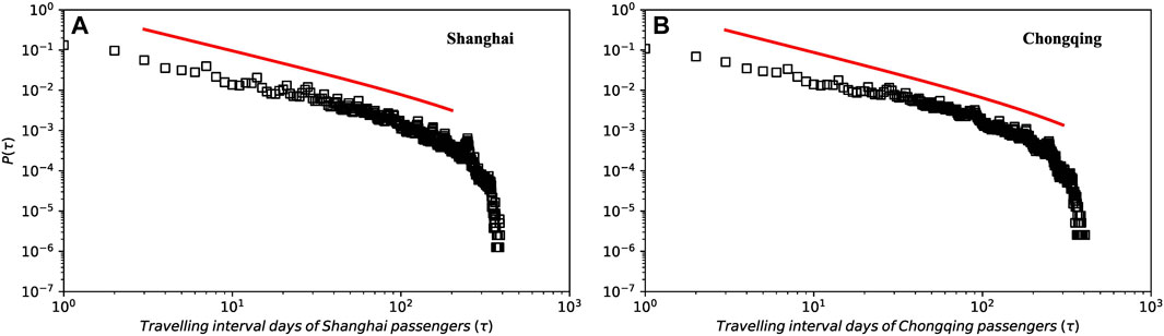
FIGURE 1. Distributions of travelling interval time.

According to the discovery of Huang [13] and Yan [19], the function of the curve of power-law with a cutoff index is shown as the following:

$P\left(\tau \right)={\tau }^{-\alpha }{e}^{-\beta \tau },(1)$

Where $\tau$ represents the inter-event time of an individual’s travelling event, and $\alpha$ represents a coefficient, and ‘e’ represents the natural constant, and $\beta$ represents a coefficient.

The parameters of the distribution function of the two datasets are calculated by maximum likelihood estimation [20]. Two functions are obtained by computer fitting, which are $P\left(\tau \right)\propto {\tau }^{-1.01}{e}^{-0.002\tau }$ (Dataset Shanghai), and $P\left(\tau \right)\propto {\tau }^{-1.05}{e}^{-0.002\tau }$ (Dataset Chongqing). The distribution diagram is shown in Figure 1, and the truncated power-law tail indicates that the travelling time intervals of passengers are not uniformly distributed.

2.2.2 Burstiness and memory

To analyze an individual’s behavior, the first step is to obtain the time of the behavior events, and then sort them into time series in order. Finally, these two indicators, the burstiness and the memory [7], are used to analyze. We use the same process and indicators to analyze the collective behavior of passengers who take intercity buses.

For a passenger, we get his boarding time for each travelling, and calculate the time series of travelling inter-event time. That is $\left\{{\tau }_1,{\tau }_2,...,{\tau }_{j{n}_j}\right\}$, then we could figure out the mean value $m_{{\tau }_j}$ and the standard deviation value ${\sigma }_{{\tau }_j}$. According to the research results of other scholars [7], the burstiness $B_j$ can be calculated by the following equation:

$B_j\equiv \frac{\left({\raisebox{1ex}{${\sigma }_{{\tau }_j}$}\!\left/ \!\raisebox{-1ex}{$m$}\right.}_{{\tau }_j}-1\right)}{\left({\raisebox{1ex}{${\sigma }_{{\tau }_j}$}\!\left/ \!\raisebox{-1ex}{$m$}\right.}_{{\tau }_j}+1\right)}=\frac{{\sigma }_{{\tau }_j}-m_{{\tau }_j}}{{\sigma }_{{\tau }_j}+m_{{\tau }_j}},(2)$

where $m_{{\tau }_j}$ and ${\sigma }_{{\tau }_j}$ are the mean and standard deviation value. It can be seen from Eq. 2 that the value of $B_j$ ranges from -1 to 1.

For passenger, calculating the time difference between the two continuous travelling events (the $\left(i+1\right)th$ , the $th$ ), can get the inter-event time, and define it as ${\tau }_{j,i}$. We can obtain the ${\tau }_{j,i}$ value of each passenger, then get a dataset, and calculate the mean $m_1$ and standard deviation ${\sigma }_1$ of this data set. By the same token, for passenger, calculate the time difference between the two continuous travelling events (the $\left(i+2\right)th$, the $\left(i+1\right)th$), and define it as ${\tau }_{j,i+1}$, then calculate and get the mean $m_2$ and standard deviation ${\sigma }_2$. The memory $M_j$ of a passenger $j$ can be calculated by the following equation:

$M_j\equiv \frac{1}{n_j-1}{\sum }_{i=1}^{n_j-1}\frac{\left({\tau }_{j,i}-m_1\right)\left({\tau }_{j,i+1}-m_2\right)}{{\sigma }_1{\sigma }_2},(3)$

where $n_j$ represents the boarding times of a passenger $j$, ${\tau }_{j,i}$ is the inter-event time between the two continuous travelling events (the $\left(i+1\right)th$ , the $ith$), and $m_1$, ${\sigma }_1$ are the mean, standard deviation value; ${\tau }_{j,i+1}$ is the inter-event time between the two continuous travelling events (the $\left(i+2\right)th$ , the $\left(i+1\right)th$), and $m_2$, ${\sigma }_2$ are the mean, standard deviation value.

It can be seen from Eq. 3 that the value of $M_j$ ranges from -1 to 1. When $M_j$ equals 0, it represents that there is no memory effect; When $M_j$ is positive, it shows that for the passenger $j$, in his travelling event time series, long inter-event time or short inter-event time continuously appears, and it’s called memory effect. When $M_j$ is negative, which indicates that in the passenger’s travelling event time series, a long inter-event time alternates with a short inter-event time, and it’s called negative memory effect.

According to the above calculation methods, from the collective behavior level, Figure 2 plots the distribution curve for these two datasets. In Figure 2, we can find the burstiness mean $B=0$ in the Shanghai dataset, the burstiness mean $B=-0.05$ in the Chongqing dataset, and the memory mean $M=-0.5$ in these two datasets. The distribution in Chongqing presents a weak burstiness. Negative memory indicates that the travelling time intervals of passengers show the situation of separation between a long time interval and a short time interval. This is very consistent with the current situation. Passengers go out by intercity bus and return by bus in a few days. Generally speaking, passengers take intercity buses for medium and long-distance travel, so the frequency of passengers taking the intercity bus cannot be as high as that of passengers taking the bus in the city at the same time. Usually, passengers will travel by intercity bus again at a long interval.

FIGURE 2

FIGURE 2. Distribution graphs (burstiness B and memory M of the Shanghai and Chongqing datasets).

2.2.3 Analysis of inter-event time between ticket purchase time and travel time

Whether to purchase tickets in advance is closely related to the passenger’s situation, such as whether the trip is planned, or whether the trip is decided suddenly and not planned. So the number of days, that is, the inter-event time between ticket purchase time and travel time, is an essential temporal feature of our analysis and research.

The distribution of advance ticket days for bus passengers in Shanghai and Chongqing is demonstrated in Figure 3.

FIGURE 3

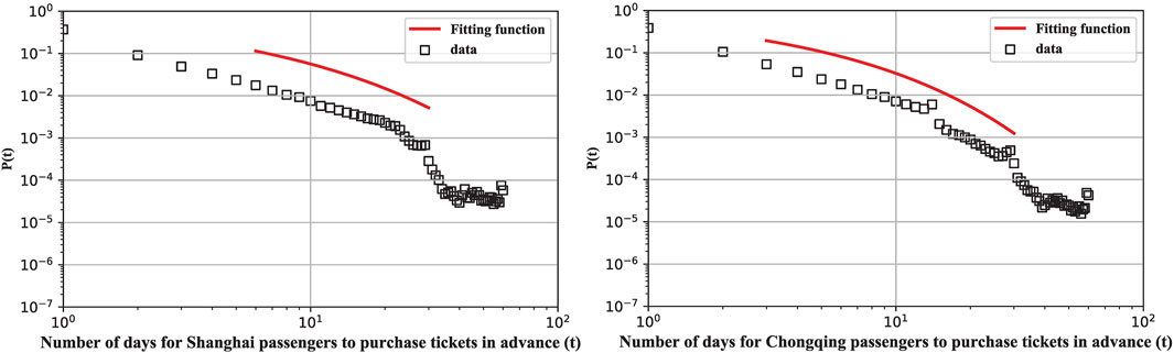
FIGURE 3. The distribution of advance ticket days to passengers in Shanghai (Chongqing) dataset.

In Figure 3, the abscissa $t$ represents the inter-event time (unit: day) between the time when a passenger books tickets and the passenger’s boarding time. The ordinate $p\left(t\right)$ represents the probability.

Based on the preliminary studies, we use the stretched exponential distribution [13] to fit the function, which is $\left(t\right)=e^{\lambda t^{\beta }}$. The fitting function of the Shanghai dataset is $\left(t\right)=e^{-0.81t^{0.55}}$ , and the fitting function of the Chongqing dataset is $p\left(t\right)=e^{-0.84t^{0.61}}$. It can be found that the parameters of the two fitting functions are very close.

It can be seen from Figure 3 that the advance ticket days of passengers are concentrated in 1–60 days, which may be related to the reservation time limit of bus tickets. Whether in Shanghai or Chongqing, the probability of passengers purchasing tickets in advance reaches its highest value on 1 day and generally decreases with the increase of ticket purchasing days in advance. There are similar dynamics for advance ticket purchase time of bus passengers in these two cities.

Traditionally, the bus ticket price does not change as frequently as the price of airline tickets. Passengers who book bus tickets do not have an awareness of saving money by buying tickets in advance. However, the number of days to purchase tickets in advance can reflect the planning and urgency of passengers’ travel purposes to a certain extent. It can reflect the types of passengers on this basis.

Passengers who buy tickets many days in advance may have travel plans, while those who book tickets in a hurry to travel may have sudden events related to work to deal with. Therefore, passengers who buy tickets in advance for a long time mostly travel on holidays and rest days. On the contrary, passengers who purchase tickets in advance for a short time mostly travel on working days.

To prove our guess, we divide the types of travel dates of passengers into three categories, which are holiday, weekend, and workday, and then explore whether there is any difference in the time of ticket purchase in advance in different types of travel dates. Limited by the time tickets can be booked, passengers can book tickets 30 days in advance at the earliest. We plot the percentage stacked bar chart of these two factors, consisting of the types of travel dates and the days of advance ticket purchase for bus passengers in the two cities, illustrated in Figure 4.

FIGURE 4

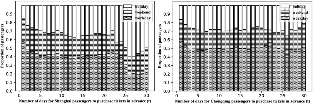
FIGURE 4. The percentage stacked bar chart of advance ticket purchase time and type of travel date in Shanghai (Chongqing) dataset.

The abscissa $t$ represents the number of days that passengers have purchased tickets in advance, and the ordinate represents the percentage. The Blank columns represent that the passengers travel in holiday; the columns filled with horizontal lines represent that the passengers travel at weekends; the column filled with crosses represents that the passengers travel on working days.

2.3 Spatial features analysis

2.3.1 Analysis of travel distance distribution

Travel distance has been widely studied in infrastructure networks such as public transportation [21]. Based on bus passenger survey data in Shijiazhuang city, Wang et al. [22] counted the passengers’ travelling distance by bus, and found that it obeyed the exponential distribution.

We compare and analyze the travel distance distribution of bus passengers and the route distance distribution of intercity bus stops in these two cities. The travel distance distribution of bus passengers in the two cities is shown in Figure 5. Here, the travel distance refers to the distance between the starting stop and the terminal stop of each passenger’s bus route.

FIGURE 5

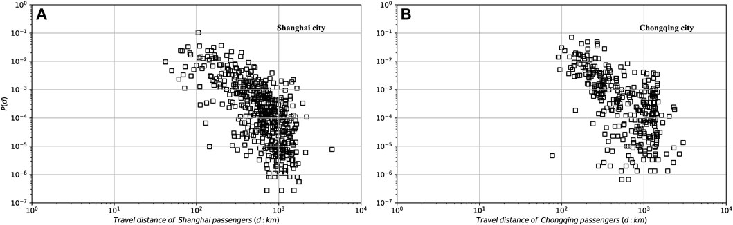
FIGURE 5. Distribution of passengers’ travelling distance.

In Figure 5, the abscissa $d$ represents in these two cities, passengers’ travelling distance, and the ordinate $p\left(d\right)$ represents probability.

According to Figure 5, most passengers in the two cities travel 100–1000 km, and some passengers in Shanghai travel less than 100 km, which may be because the distance between Shanghai and the surrounding cities of Shanghai is less than 100 km.

Since the travel distance of bus passengers is heavily dependent on the route distance operated by the bus company, we break up the length of distance into intervals and then plot the compound bar chart of travel distance and bus route distance, which is demonstrated in Figure 6.

FIGURE 6

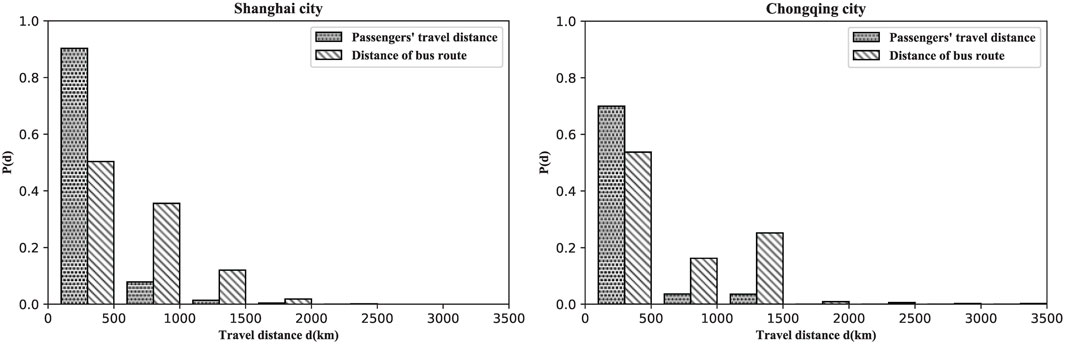
FIGURE 6. The compound bar chart of travel distance and bus route distance in Shanghai (Chongqing) dataset.

In Figure 6, the abscissa $d$ represents the distance, and the ordinate represents probability. The columns filled with crosses represent the distribution of travel distance by passengers, and the columns filled with slashes represent the distribution of travel distance of bus routes operated by bus companies.

In Figure 6, we can find that for the highest column, the corresponding abscissa axis is between 0 and 500 km. Moreover, it can be seen that the height of the two types of columns is quite different. In the range of 0–500 km, the travel distance distribution probability of passengers is even much higher than that of bus routes. In the Shanghai city sub-picture, for the distance of bus routes, the proportion of 0–500 km is not much different from that of 500–1000 km, but the probability of passenger travel distance distribution in the range of 0–500 km is close to 0.9, and the probability of passenger travel distance distribution in the range of 500–1000 km is close to 0.1. The probability of passenger travel distance distribution in the field of 0–500 km is also close to 0.9 in Chongqing.

We guess that the intercity bus is the preferred means of transportation for passengers for short and medium-distance travel. For long-distance travel, passengers may choose high-speed rail or an airplane with a high probability. However, it can be seen that the number of long-distance buses and medium and short distance buses is unreasonable. The number of short-distance intercity buses should be increased to meet the passengers’ demand.

According to Figure 5 and Figure 6, as the travel of bus passengers depends on the bus route transportation network, the travel distance distribution of bus passengers exhibits scale-free features. Brockmann et al. [9] studied the flow trajectory of banknotes as the banknotes were traded in different hands, and the flow distance of banknotes was not limited to the transportation network, so distance distribution obeyed the power law.

2.3.2 Cyclotron radius and mean square displacement

In the study of human mobility features, the diffusion features of humans can be represented by the growth law of the cyclotron radius and the mean square displacement (MSD) with time. The cyclotron radius [10] of all bus passengers in each city after n trips is given as:

$r_g\left(n\right)=\sqrt{\frac{1}{n}{\displaystyle \sum }_{k=1}^n{\left(x_k-x_t\right)}^2},(4)$

Where $x_t$ represents the bus stop visited by all bus passengers most times on $n$ trips, and $x_k$ represents the bus stop that the passengers arrive at on each trip, and $x_k-x_t$ represents the distance between the two bus stops. In particular, for a passenger who only travels once, $x_t$ and $x_k$ denote the departure stop and the arrival stop of the bus route.Where, the abscissa $n$ represents the travelling times of passengers, and the ordinate $r_g\left(n\right)$ represents the cyclotron radius.

In Figure 7, the overall cyclotron radius of bus passengers in the two cities reaches its maximum when the number of trips is 1. In the Shanghai data set, with the increase in the number of trips, the cyclotron radius decreases sharply. Until the number of trips n equals 28, the cyclotron radius begins to stabilize, at close to 100 km. In the Chongqing data set, when n ranges from 2 to 7, the cyclotron radius decreases slowly; when n ranges from 7 to 20, the cyclotron radius is relatively stable; and when n is greater than 20, the cyclotron radius is more divergent.

FIGURE 7

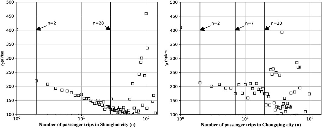
FIGURE 7. Distribution of cyclotron radius in Shanghai (Chongqing) dataset.

When the number of trips of bus passengers equals 1, the cyclotron radius is the largest, because when n equals 1, many passengers only travel once. Their cyclotron radius is the actual travel distance. When n is greater than 1, their round-trip rate is also very high. That is to say, when a passenger arrives at the destination bus stop, there is a high probability that he will return to the previous bus stop where he departed last, which results in the passengers’ cyclotron radius decreasing rapidly.

In the Shanghai dataset, for passengers who travel 2–28 times, their destination cities are relatively close. Their travel frequency is very high, so the cyclotron radius generally shows a trend of decreasing with the increase in the number of trips. In the Chongqing dataset, passengers who travel 7–20 times often take intercity buses, and they have relatively stable and balanced trips in the bus stop network. The cyclotron radius decreases when the travelling times increase. Therefore, the features are different from those of other types of passengers.

The MSD distribution of bus passengers is shown in Figure 8. The MSD is given as:

$MSD\left(n\right)=\langle {\left(x_n-x_0\right)}^2\rangle ,(5)$

Where $x_0$ is the location of the first departure bus stop in the passenger’s travel record, and the $\langle •\rangle$ operator refers to the mean distance of $n$ trips.Where, the abscissa $n$ represents passengers’ travelling times in each city, and the ordinate represents the MSD of the passengers’ trips. In Figure 8, the MSD has a peak value at the beginning. When $n$ ranges from 1 to 18 (19), the MSD shows a downward trend. After that, the number of trips continues to increase, and the MSD presents a discrete distribution.

FIGURE 8

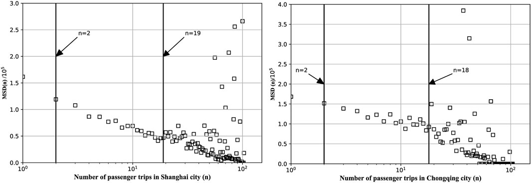
FIGURE 8. Distribution of MSD in Shanghai (Chongqing) dataset.

According to the previous analysis of the cyclotron radius and the MSD, we can see that the cyclotron radius and MSD of passengers’ trips are closely related to the number of trips. The travel distance of most passengers does not increase with the increase in the number of trips but changes within a specific range, indicating the high boundedness of bus passenger trips. The distribution of the cyclotron radius in the Shanghai and Chongqing datasets is quite different. It is speculated that there are more passengers travelling for short distances in the surrounding areas of Shanghai, and they travel frequently. So the cyclotron radius decreases steadily with the increase in the number of trips.

2.4 Proportion of passenger trips per month

We counted the number of trips of all passengers in Shanghai (Chongqing) dataset in each month of the year, and the proportion of passenger trips per month in these two cities in year 2019 is shown in Figure 9.

FIGURE 9

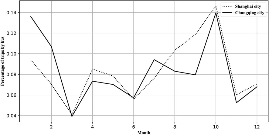
FIGURE 9. The proportion of passenger trips per month.

The abscissa in Figure 9 represents the month, and the ordinate represents the proportion of passenger trips per month.

The spring Festival holiday in 2019 was from February 4 to February 10. Before the spring Festival, many passengers needed to take the intercity bus to go home, and in October, many passengers would travel on the National day. Therefore, January and October were the two periods with the highest passengers. April 5 to April 7 in 2019 was the Qingming Festival, and some passengers travelled during this period. However, during the period from July to October, the proportion of passengers in the two cities showed different trends. According to the data set from Chongqing, the travel volume of passengers was higher in July and continued to decrease in August and September. In the data set for Shanghai, the travel volume of passengers continued to rise from July to September. This period coincided with the summer vacation of students. It was speculated that during this period, many passengers with their children travelled to Shanghai and took intercity buses to travel to the cities around Shanghai. It also indicates that during festivals and summer holidays, bus companies should adjust their operation plans and increase the number of buses to meet the strong travel demand of passengers.

As shown in Figure 9, in January and October, the proportion of passenger trips was the highest in these two cities. We further analyzed the travel distance distribution of passengers in the two cities in these 2 months, as shown in Table 2. In Table 2, we can find that in Shanghai, the proportion of trips below 500 km is 88% in October and 78% in January; In Chongqing, the proportion of trips below 500 km is 93% in October and 88% in January, and this indicates that in October, passengers in Shanghai and Chongqing are more inclined to travel for short distances.

TABLE 2

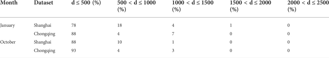
TABLE 2. Travel distance ratio (d, unit: km) in January and October in Shanghai and Chongqing.

In Table 2, at least 80% of the travel distance is less than 500 km, so we listed the proportion of travel distance below 500 km, which is shown in Table 3. According Table 3, we can find that in Chongqing, at least 70% of the travel distance is between 100 km and 300 km, and this may be due to that there is a strong demand for short-distance travel around the city, and Chongqing has a larger area than Shanghai.

TABLE 3

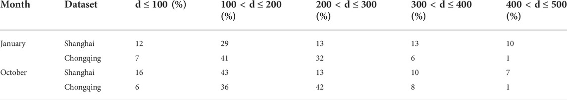
TABLE 3. Travel distance ratio (d ≤ 500, unit: km) in January and October in Shanghai and Chongqing.

3 Discussions

From the results of the experimental analysis, the passengers’ travelling interval time presents a power-law curve with a cutoff index, and both exhibit weak burstiness and strong negative memory effects. Passengers take the intercity bus to go out and return in a few days. After a long period, the passengers will travel by intercity bus again, so the travelling time intervals of passengers present the situation that a long inter-event time alternates with a short inter-event time, which shows a negative memory effect.

There are similar dynamics for advance ticket purchase time of bus passengers in these two cities. When travelling on holiday, they prefer to buy tickets in advance in Shanghai. According to the analysis of the date of purchase of tickets in advance and the type of travel date, in Shanghai, among those who purchase tickets 25–30 days in advance, more than 50% of passengers plan to travel on holidays. Maybe these passengers are worried that they can’t buy tickets near holidays. Therefore, on holidays, the transportation department and bus operation company should increase the amount of transportation.

The bus route network limits the travel distance of passengers. The distribution of travel distance of passengers by intercity bus in the two cities does not have scale-free features, which is more in line with the stretching index distribution.

According to the distribution of travel distance and bus route distance, in Shanghai and Chongqing, there is a strong demand for medium and short-distance travel within 500 km. In comparison, there is less demand for long-distance travel above 500 km. So the transportation departments and bus operation companies in the two places should adjust the bus routes, and concentrate the traffic on short-distance routes within 500 km.

The cyclotron radius and the MSD of passengers’ travelling distance, which indicate that the mobility distance of most passengers does not increase infinitely with the increase of the number of trips and changes within a specific range. The two groups of bus passengers tend to move in a limited range, and their travel distance is highly bounded. There is a big difference in the distribution of the cyclotron radius of travel between the two groups. There are more short-distance passengers to and from Shanghai, so the cyclotron radius decreases steadily with the increase in the number of trips in the Shanghai dataset.

Holiday factors have a significant impact on the travel of the two groups, mainly traditional festivals such as spring Festival, Qingming Festival, and National Day. During these periods, the number of passengers travelling is large. The number of passengers travelling to and from Shanghai in the summer gradually increases. According to the proportion of passengers travelling in 1 year, in the two cities, passengers travel mainly in January and October, so the transportation department can consider increasing the amount of transportation in these two time periods.

4 Conclusion

The passengers’ travelling inter-event time by taking the intercity bus presents a power-law with a cutoff index, and both exhibit weak burstiness and strong negative memory effects. The distribution of travel distance of passengers by intercity bus in the two cities does not have scale-free features, which is more in line with the stretching index distribution. The difference in cyclotron radius between these two groups’ travelling distances is quite significant; roundtrips from Shanghai are frequent. Holidays have a significant influence on passengers’ travel behaviors, which leads to more trips.

In terms of application, the transportation department and bus operation company can optimize the intercity bus operation and adjust their operation strategy based on the suggestions in this paper.

The travelling time intervals of passengers in the two cities show low burstiness and negative memory effects, and the underlying principles need to be further explored. In terms of theory, the results in this paper can provide help for more scholars’ research to study the features of human mobility behaviors.

Data availability statement

The original contributions presented in the study are included in the article/supplementary material, further inquiries can be directed to the corresponding author.

Author contributions

S-YH provided this topic and wrote the manuscript. J-CZ, C-HX and ZW guided, discussed, and modified the manuscript. All authors contributed to the manuscript and approved the submitted version.

Funding

Supported by a project grant from Zhejiang Philosophy and Social Sciences Foundation (Grand No.19NDJC145 YB).

Conflict of interest

Author S-YH was employed by Bank of Zhengzhou.

The remaining authors declare that the research was conducted in the absence of any commercial or financial relationships that could be construed as a potential conflict of interest.

Publisher’s note

All claims expressed in this article are solely those of the authors and do not necessarily represent those of their affiliated organizations, or those of the publisher, the editors and the reviewers. Any product that may be evaluated in this article, or claim that may be made by its manufacturer, is not guaranteed or endorsed by the publisher.

References

1. Barabasi AL. The origin of bursts and heavy tails in human dynamics. Nature (2005) 435(7039):207–11. doi:10.1038/nature03459

PubMed Abstract | CrossRef Full Text | Google Scholar

2. Guo JL. A model of human behavior dynamics and exact results. Acta Phys Sin (2010) 59(6):3851–5. doi:10.7498/aps.59.3851

CrossRef Full Text | Google Scholar

3. Yan XY, Zhao C, Fan Y, Di ZR, Wang WX. Universal predictability of mobility patterns in cities. J R Soc Interf (2014) 11(100):20140834. doi:10.1098/rsif.2014.0834

PubMed Abstract | CrossRef Full Text | Google Scholar

4. Zhou T, Han XP, Yan XY, Yang ZM, Zhao ZD, Wang BH. Statistical mechanics on temporal and spatial activities of human. J Univ Electron Sci Tech China (2013) 42(4):481–540. doi:10.3969/j.issn.1001-0548-2013.04.001

CrossRef Full Text | Google Scholar

5. Dezsö Z, Almaas E, Lukács A, Rácz B, Szakadát I, Barabási AL. Dynamics of information access on the web. Phys Rev E (2006) 73(6):066132. doi:10.1103/PhysRevE.73.066132

CrossRef Full Text | Google Scholar

6. Zhou T, Kiet HAT, Kim BJ, Wang BH, Holme P. Role of activity in human dynamics. Europhys Lett (2008) 82(2):28002. doi:10.1209/0295-5075/82/28002

CrossRef Full Text | Google Scholar

7. Goh KI, Barabási AL. Burstiness and memory in complex systems. Europhys Lett (2008) 81(4):48002. doi:10.1209/0295-5075/81/48002

CrossRef Full Text | Google Scholar

8. Lambiotte R, Tabourier L, Delvenne JC. Burstiness and spreading on temporal networks. Eur Phys J B (2013) 86(7):320–4. doi:10.1140/epjb/e2013-40456-9

CrossRef Full Text | Google Scholar

9. Brockmann D, Hufnagel L, Geisel T. The scaling laws of human travel. Nature (2006) 439(7075):462–5. doi:10.1038/nature04292

PubMed Abstract | CrossRef Full Text | Google Scholar

10. Gonzalez MC, Hidalgo CA, Barabasi AL. Understanding individual human mobility patterns. nature (2008) 453(7196):779–82. doi:10.1038/nature06958

PubMed Abstract | CrossRef Full Text | Google Scholar

11. Song C, Qu Z, Blumm N, Barabási AL. Limits of predictability in human mobility. Science (2010) 327(5968):1018–21. doi:10.1126/science.1177170

PubMed Abstract | CrossRef Full Text | Google Scholar

12. Sun YF, Gan HC. Car commuters' travel behaviors with presence of multi-modal travel information. J Univ Shanghai Sci Tech (2018) 40(6):595–600. doi:10.13255/j.cnki.jusst.2018.06.013

CrossRef Full Text | Google Scholar

13. Huang FH, Peng J, You MY. Analyses of characetristics of air passenger group mobility behaviors. Acta Phys Sin (2016) 65(22):228901–328. doi:10.7498/aps.65.228901

CrossRef Full Text | Google Scholar

14. Yang G, Battie MC, Boyd SK, Videman T, Wang Y. Cranio-caudal asymmetries in trabecular architecture reflect vertebral fracture patterns. Bone (2017) 3:102–7. doi:10.1016/j.bone.2016.11.018

PubMed Abstract | CrossRef Full Text | Google Scholar

15. Tao S. Spatial-temporal analysis of travel behaviour using transit smart card data and its planning implications: A case study of Brisbane, Australia. Shanghai Urban Plann Rev (2017) 5:94–9. doi:10.11982/j.supr.20170594

CrossRef Full Text | Google Scholar

16. Han SY, Guo Q, Yu K, Li RD, He B, Liu JG. Statistical mechanism of passenger mobility behaviors for different transportations. Int J Mod Phys C (2020) 31(6):2050082–13. doi:10.1142/S0129183120500825

CrossRef Full Text | Google Scholar

17. Cai SL, Li SC. An analysis on location of chongqing city. J Sichuan Normal Univ (Natural Science) (2001) 24(4):423–5. doi:10.3969/j.issn.1001-8395.2001.04.030

CrossRef Full Text | Google Scholar

18. Chen J, Chen Q, Li HP. Psychological influences on bus travel mode choice: A comparative analysis between two Chinese cities. J Adv Transportation (2020) 2:1–9. doi:10.1155/2020/8848741

CrossRef Full Text | Google Scholar

19. Yan XY, Han XP, Wang BH, Zhou T. Diversity of individual mobility patterns and emergence of aggregated scaling laws. Sci Rep (2015) 34(4):2678. doi:10.1038/srep02678

PubMed Abstract | CrossRef Full Text | Google Scholar

20. Zhao H, Zhang C. Maximum likelihood estimation for reflected Ornstein-Uhlenbeck processes with jumps. Commun Stat - Theor Methods (2019) 48(5):1221–33. doi:10.1080/03610926.2018.1425451

CrossRef Full Text | Google Scholar

21. Peng CB, Jin XG, Wong KC, Shi MX, Liò P. Collective human mobility pattern from taxi trips in urban area. PloS one (2012) 7(4):e34487. doi:10.1371/journal.pone.0034487

PubMed Abstract | CrossRef Full Text | Google Scholar

22. Wang MS, Huang L, Yan XY. Exploring the mobility patterns of public transport passengers. J Univ Electron Sci Tech China (2012) 41(1):2–7. doi:10.3969/j.issn.1001-0548.2012.01.001

CrossRef Full Text | Google Scholar