Resembling the bottleneck effect in p53 core network including the dephosphorylation of ATM by Wip1: A computational study

As one of the key proteins, wild-type p53 can inhibit the tumor development and regulate the cell fate. Thus, the study on p53 and its related kinetics has important physiological significance. Previous experiments have shown that wild-type p53-transcribed phosphatase one protein Wip1 can maintain the continuous oscillation of the p53 network through post-translational modification. However, the relevant details are still unclear. Based on our previous p53 network model, this paper focuses on the modification of Wip1 dephosphorylated ataxia telangiectasia mutant protein ATM. Firstly, the characteristics and mechanism of p53 network oscillation under different numbers of DNA double strand damage were clarified. Then, the influence of ATM dephosphorylation by Wip1 on network dynamics and its causes are investigated, including the regulation of network dynamics transition by the mutual antagonism between ATM dephosphorylation and autophosphorylation, as well as the precise regulation of oscillation by ATM-p53-Wip1 negative feedback loop. Finally, the cooperative process between the dephosphorylation of ATM and the degradation of Mdm2 in the nucleus was investigated. The above results show that Wip1 interacts with other components in p53 protein network to form a multiple coupled positive and negative feedback loop. And this complex structure provides great feasibility in maintaining stable oscillation. What’s more, for the state of oscillation, the bottleneck like effect will arise, especially under a certain coupled model with two or more competitive negative feedback loops. The above results may provide some theoretical basis for tumor inhibition by artificially regulating the dynamics of p53.

1 Introduction

As the basic unit of life, cells can regulate their own behavior to adapt to intra- and extracellular stress signals, depending on the protein interaction networks [1]. The p53 signaling network, with protein p53 at its core, is one of the key components of the cell, being a popular research topic in physiology for the last 4 decades [2–4]. Studies have shown that p53 is strongly associated with many types of cancer, such as liver, lung, breast, stomach, colon and prostate cancers [4–6]. To mitigate threatens from these troubles, there is an urgent need to improve the understanding of p53. In resting state, the E3 ubiquitin ligase Murine Double Minute 2 (Mdm2) can promote rapid degradation of p53, resulting in low p53 expression levels [7]. Under stressful conditions, such as ionizing radiation, UV irradiation, drug induction or metabolic stress, p53 is activated and maintained at high levels [8–11]. As a multifunctional transcription factor, p53 can induce the expression of various downstream proteins involved in the cell cycle, metabolism or apoptosis [12, 13]. In particular, for cell fate decision, p53 dynamics are showing great effect in different environments [14–16]. Studies have shown that pulsed oscillations in the p53 network are widespread [17, 18], determining the survival probability of cell, and it needs to be studied in detail. Therefore, the generation and maintenance of stable oscillations deserves further investigation. What’s more, the related process in oscillation like gene transcription and protein post-translational modifications, which can form coupled multi-feedback loops, still needs to be investigated. In this paper, we focus on the phosphorylation and dephosphorylation of the ataxia-telangiectasia mutated protein (ATM) at site of Ser1981 [19, 20] and provide insight into the dynamics of the associated p53 signaling network.

Induced by ionizing radiation or drugs, undamped periodic oscillations in single cells or cell populations are the typical feature of protein p53, in which the radiation doses are correlated with the number of oscillatory pulses [21, 22]. For this phenomenon, many theoretical models have been established, which are based on the p53-Mdm2 negative feedback loop [22] (NFL). For example, the model designed by [23], including the p53-Mdm2 NFL as the main structure, has investigated the global stability of p53 network. Based on the NFL of p53-Mdm2, some models considered multiple NFLs, such as the models in Refs. [18, 24], which added the NFL of p53-Wip1-ATM to investigate the stable, oscillations and biorhythms in the signaling transduction network; the Yang’s model [25], which examined the phosphorylation of the Ser395 site of Mdm2, analyzed the coupled positive feedback loop (PFL) and NFL of p53-Mdm2 and related kinetics; the Ouattara’s model [26], which distinguished the nucleus and cytoplasm of p53, found the amplitude and height of p53 were variable, while the peak width and period were less affected by noise. In addition to these deterministic models, stochastic kinetic models have also been widely used, e.g., the model constructed by Ma et al. [27] includes differential equations and stochastic repair processes to reproduce the pulsing release behavior of p53; the model by Xia and Jia [28] includes a p53 oscillation module and a DNA repair module, successfully explained the possible mechanism of ion radiation dose regulation of the p53 pulse number. Another stochastic model [29] introduced the τ-leap algorithm to reproduce the response details of the p53 protein network and discusses the effects of intra/extracellular noise and cellular variability on the stability of oscillations. These models provided a comprehensive analysis of p53-related dynamics and yield important results. However, some details of the network still need to be investigated in depth, e.g., how to regulate the single feedback loop, coupled positive and negative feedback loops [30–33] or coupled double NFLs within the structure of co-existence of multiple feedback loops.

In order to answer these questions, this paper takes the phosphorylation and dephosphorylation processes of ATM as a starting point, and investigates the changes of p53 network dynamics. Basing on a simple p53 network structure, the kinetic equations of the model are given. Then, through numerical analysis, the relationship between the network system and the degree of damage and other parameters is found, and the bifurcation point and the state characteristics of the system are clarified; together with the bifurcation curve, the oscillation region on the two-parameter bifurcation diagram can be determined. Numerical analysis showed that the different response patterns of the cells under UV and IR radiation were closely related to the strength of the positive feedbacks and negative feedbacks [34] on ATM, indicating that dephosphorylation of Wip1 is a critical part of the network and its presence increases the regulatory pathway. The computational results show that the negative feedback of p53-Mdm2 is fundamental to the oscillations of the p53 network, while other feedbacks have a regulatory effect on the p53 oscillations and can maintain the stability of the oscillations. In conclusion, the model demonstrates that the p53 oscillations occur as a result of the coupling and compromise between NFL and PFL/NFL in close proximity to each other. In contrast to the conclusions of other models, we believe that the antagonistic strengths acting on different components of the same loop need to be of the same magnitude, and the strengths of the coupled positive and negative feedbacks in different loops need to be matched, and the formation of a competitive relationship between the coupled double negative feedbacks needs to be coordinated.

2 Model and methods

2.1 Model

2.1.1 The p53 core network model

Based on previous studies [15, 16, 24, 29], we constructed a simplified model containing the core components associated with p53 oscillations, as shown in Figure 1. The model takes into account the action of ionizing radiation (IR) or DNA damage agents [35] (e.g., etoposide). The DNA double strand break (DSB) occurs and DNA repair proteins are then recruited to repair the damage. At the same time, rapid autophosphorylation of ATM is induced in cells [36], causing the conversion of ATM dimers (ATM₂) into active phosphorylated ATM monomers (ATM_p) [36, 37]. ATM_p further phosphorylates p53 and Mdm2, accelerates the degradation of nuclear Mdm2, and enhances the stability and transcriptional activity of p53 [37]. In non-stressed cells, p53 remains at a low level due to the negative regulation of the E3 ubiquitin ligase Mdm2. However, the p53 protein concentration can be maintained at high levels at this time. Phosphorylation of p53 (p53_p) induces the production of Mdm2 and Wip1 [19], while Wip1 dephosphorylates p53 and ATM_p. In the abstract, there are two negative feedbacks and one positive feedback in the model. Practical experiments have shown that p53 oscillations can last for a long time [23]. Considering that DNA damage repair may be defective in some cells, the repair process is not added to the model and the initial number of DNA damages is used as input.

FIGURE 1

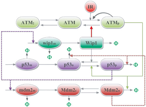
FIGURE 1. Schematic diagram of the p53 protein network model. After irradiation, DNA damage activates ATM, which can phosphorylate and accelerate the degradation of nuclear Mdm2, thereby stabilizing and activating p53 phosphorylation. Then, p53 will induce the production of Mdm2 and Wip1, while Wip1 can dephosphorylate ATM and p53 in turn. The symbol Φ represents the degradation process.

2.1.2 Deterministic equations

The dynamics of the model is described by a system of ordinary differential equations (ODES). The kinetic equations for ATM activation are as follows.

$\frac{\mathrm{d}\left[{\mathrm{A}\mathrm{T}\mathrm{M}}_2\right]}{\mathrm{d}t}=k_{\dim }\cdot {\left[\mathrm{A}\mathrm{T}\mathrm{M}\right]}^2-k_{\text{udim}}\cdot \left[{\mathrm{A}\mathrm{T}\mathrm{M}}_2\right],(1)$

$\begin{array}{ll}\hfill \frac{\mathrm{d}\left[{\mathrm{A}\mathrm{T}\mathrm{M}}_{\text{p}}\right]}{\mathrm{d}t}& =k_{\text{basal}}\cdot H^{+}\left(\left[\mathrm{A}\mathrm{T}\mathrm{M}\right],j_{\text{atms}}\right)-k_{\text{deatm}}\cdot H^{+}\left(\left[{\mathrm{A}\mathrm{T}\mathrm{M}}_{\text{p}}\right],j_{\text{deatm}}\right)\hfill \\ \hfill & +k_{\text{acatm}}\cdot \left[{\mathrm{A}\mathrm{T}\mathrm{M}}_{\text{p}}\right]\cdot \frac{N_{\text{dsb}}}{N_{\text{dsb}}+j_{\text{dsb}}}\cdot H^{+}\left(\left[\mathrm{A}\mathrm{T}\mathrm{M}\right],j_{\text{acatm}}\right)\hfill \\ \hfill & -k_{\text{deatmwip}}\cdot \left[\mathrm{W}\mathrm{i}\mathrm{p}\mathrm{1}\right]\cdot H^{+}\left(\left[{\mathrm{A}\mathrm{T}\mathrm{M}}_{\text{p}}\right],j_{\text{deatmwip}}\right).\hfill \end{array}(2)$

Where, [−] represents the concentration of the component, the function H⁺(A,B) is defined as A/(A+ B). It has been shown that the total amount of ATM does not change much after IR [19], so [ATM]_tot = [ATM] + [ATM_p] + 2 [ATM₂] is a constant in the model. The binding and dissociation reactions of proteins in the model are described by the law of mass action, while the enzymatic reactions are characterized by Michaelis-Menten kinetics (MM). In undamaged cells, ATM appears as dimers or oligomers. And the ATM dimer can spontaneously polymerize or dissociate into inactive monomers, of which the reaction intensity is reflected by k_dim and k_udim correspondingly. After DNA damage, ATM dimmers are recruited to the damaged DNA and the ATM autophosphorylation [20] will be accelerated, involving the basal activation and the DNA damages induced activation, of which the strengths are represented by k_basal and k_acatm respectively. The process is summarized by the first and third term on the righ-hand side of Eq. 2, where N_dsb represents the amount of DNA damage.

The p53-related kinetics include the basic transcriptional, translational, phosphorylation and reversible phosphorylation processes, as described below.

$\frac{\mathrm{d}\left[{\mathrm{p}\mathrm{53}}_{\text{m}}\right]}{\mathrm{d}t}=k_{\text{sp}53}-k_{\text{dp}53\text{m}}\cdot \left[{\mathrm{p}\mathrm{53}}_{\text{m}}\right],(3)$

$\begin{array}{ll}\hfill \frac{\mathrm{d}\left[{\mathrm{p}\mathrm{53}}_{\text{u}}\right]}{\mathrm{d}t}& =k_{\text{rp}53}\cdot \left[{\mathrm{p}\mathrm{53}}_{\text{m}}\right]+k_{\mathit{wip53s}}\cdot \left[\mathrm{W}\mathrm{i}\mathrm{p}\mathrm{1}\right]\cdot H^{+}\left(\left[{\mathrm{p}\mathrm{53}}_{\text{p}}\right],j_{\text{wip}53\text{s}}\right)-k_{\text{dep}53}\cdot \left[{\mathrm{p}\mathrm{53}}_{\text{u}}\right]\hfill \\ \hfill & -k_{\text{acp}531}\cdot \left[{\mathrm{A}\mathrm{T}\mathrm{M}}_{\text{p}}\right]\cdot H^{+}\left(\left[{\mathrm{p}\mathrm{53}}_{\text{u}}\right],j_{\text{ap}53}\right)\hfill \\ \hfill & -k_{\text{dp}53}\cdot \left[{\mathrm{M}\mathrm{d}\mathrm{m}\mathrm{2}}_{\text{n}}\right]\cdot H^{+}\left(\left[{\mathrm{p}\mathrm{53}}_{\text{u}}\right],j_{\text{p}53}\right),\hfill \end{array}(4)$

$\begin{array}{ll}\hfill \frac{\mathrm{d}\left[{\mathrm{p}\mathrm{53}}_{\text{p}}\right]}{\mathrm{d}t}& =k_{\text{acp}531}\cdot \left[{\mathrm{A}\mathrm{T}\mathrm{M}}_{\text{p}}\right]\cdot H^{+}\left(\left[{\mathrm{p}\mathrm{53}}_{\text{u}}\right],j_{\text{ap}53}\right)-k_{\text{dep}53\text{s}}\cdot \left[{\mathrm{p}\mathrm{53}}_{\text{p}}\right]\hfill \\ \hfill & -k_{\text{dp}53\text{s}}\cdot \left[{\mathrm{M}\mathrm{d}\mathrm{m}\mathrm{2}}_{\text{n}}\right]\cdot H^{+}\left(\left[{\mathrm{p}\mathrm{53}}_{\text{p}}\right],j_{\text{p}53\text{s}}\right)\hfill \\ \hfill & -k_{\text{wip}53\text{s}}\cdot \left[\mathrm{W}\mathrm{i}\mathrm{p}\mathrm{1}\right]\cdot H^{+}\left(\left[{\mathrm{p}\mathrm{53}}_{\text{p}}\right],j_{\text{wip}53\text{s}}\right).\hfill \end{array}(5)$

The Mdm2-related dynamics are stated as follows:

$\frac{\mathrm{d}\left[{\mathrm{m}\mathrm{d}\mathrm{m}\mathrm{2}}_{\text{m}}\right]}{\mathrm{d}t}=k_{\text{smdm}20}+k_{\text{smdm}2}\cdot H^{\left(+,4\right)}\left(\left[{\mathrm{p}\mathrm{53}}^{\text{p}}\right],j_{\text{smdm}2}\right)-k_{\text{dmdm}2\text{m}}\cdot \left[{\mathrm{m}\mathrm{d}\mathrm{m}\mathrm{2}}_{\text{m}}\right],(6)$

$\begin{array}{ll}\hfill \frac{\mathrm{d}\left[{\mathrm{M}\mathrm{d}\mathrm{m}\mathrm{2}}_{\text{c}}\right]}{\mathrm{d}t}& =k_{\text{rdmdm}2}\cdot \left[{\mathrm{m}\mathrm{d}\mathrm{m}\mathrm{2}}_{\text{m}}\right]-k_{\text{dmdm}2\text{c}}\cdot \left[{\mathrm{M}\mathrm{d}\mathrm{m}\mathrm{2}}_{\text{c}}\right]\hfill \\ \hfill & +k_{\text{o}}\cdot \left[{\mathrm{M}\mathrm{d}\mathrm{m}\mathrm{2}}_{\text{n}}\right]-k_{\text{i}}\cdot \left[{\mathrm{M}\mathrm{d}\mathrm{m}\mathrm{2}}_{\text{c}}\right],\hfill \end{array}(7)$

$\begin{array}{ll}\hfill \frac{\mathrm{d}\left[{\mathrm{M}\mathrm{d}\mathrm{m}\mathrm{2}}_{\text{n}}\right]}{\mathrm{d}t}& =k_{\text{i}}\cdot \left[{\mathrm{M}\mathrm{d}\mathrm{m}\mathrm{2}}_{\text{c}}\right]-k_{\text{o}}\cdot \left[{\mathrm{M}\mathrm{d}\mathrm{m}\mathrm{2}}_{\text{n}}\right]-k_{\text{dmdm}2\text{n0}}\cdot \left[{\mathrm{M}\mathrm{d}\mathrm{m}\mathrm{2}}_{\text{n}}\right]\hfill \\ \hfill & -k_{\text{dmdm}2\text{n}1}\cdot \left[{\mathrm{A}\mathrm{T}\mathrm{M}}_{\text{p}}\right]\cdot H^{+}\left(\left[{\mathrm{M}\mathrm{d}\mathrm{m}\mathrm{2}}_{\text{n}}\right],j_{\text{mdm}2\text{n}}\right).\hfill \end{array}(8)$

For Mdm2, the model considers Mdm2 in two forms: intracytoplasmic Mdm2 (Mdm2_c) and intra-nuclear Mdm2 (Mdm2_n). And the p53 transcription of mdm2_m is characterized by the Hill function with the form of H^+,n (A,B) defined as Aⁿ/(Aⁿ + Bⁿ), where n indicating the degree of synergy. The nuclear input and output Mdm2 are expressed as linear terms of the rate constant, respectively.

Similarly, the kinetic behavior of Wip1 is described by the following equation, and the transcription of Wip1 by p53 is portrayed by the Hill equation.

$\frac{\mathrm{d}\left[{\mathrm{w}\mathrm{i}\mathrm{p}\mathrm{1}}_{\text{m}}\right]}{\mathrm{d}t}=k_{\text{swip}10}+k_{\text{swip}1}\cdot H^{\left(+,3\right)}\left(\left[{\mathrm{p}\mathrm{53}}_{\text{p}}\right],j_{\text{swip}1}\right)-k_{\text{dwip}1\text{m}}\cdot \left[{\mathrm{w}\mathrm{i}\mathrm{p}\mathrm{1}}_{\text{m}}\right],(9)$

$\frac{\mathrm{d}\left[\mathrm{W}\mathrm{i}\mathrm{p}\mathrm{1}\right]}{\mathrm{d}t}=k_{\text{rwip}1}\cdot \left[{\mathrm{w}\mathrm{i}\mathrm{p}\mathrm{1}}_{\text{m}}\right]-k_{\text{dwip}1}\cdot \left[\mathrm{W}\mathrm{i}\mathrm{p}\mathrm{1}\right].(10)$

The unit of time is minute, while concentrations are divided by some certain standard concentrations, thus being dimensionless. And, all the parameters are listed in Table 1.

TABLE 1

TABLE 1. Default values of parameters.

2.2 Material and methods

p53 related network in cell lines has rich dynamics with non-linear characteristics, and the bifurcation analysis method is an effective means to probe the reason for such non-linear dynamics behaviors of cells. When the parameters of the system change, the system will undergo sudden changes, such as the transformations from stable to unstable state, the appearance of limit cycle, chaos, and so on. These changes can be called bifurcations. As a typical non-linear system model, p53 core network model has rich and complex dynamics, associating with many types of bifurcation. For example, when the protein is activated, its expression can change from a low level to a stable high level, corresponding to Saddle-Node bifurcation. If stimulated by the external signal, the protein concentration in the cell can transform from a stable equilibrium state to a limit cycle oscillation, suggesting the Hopf bifurcation. Thus, the parameters in the p53 network model can affect the non-linear dynamics greatly. To reveal the principle of how to regulate the p53 network, it is meaningful to make the bifurcation analysis.

For bifurcation analysis, such software as Oscill8 [38] and MatCont [39] are commonly used to draw the trajectory diagram of the variables when the parameters change. In this study, the Oscill8 software is introduced to make one or two parameter bifurcation analysis, while MatCont is used to check the two parameter bifurcation analysis results. In the bifurcation analysis diagrams, this study only shows the results in the case of positive values, such as the reaction rates and protein levels, and discards the negative results, although they are mathematically meaningful.

Given a fixed parameter of external inputs in the model, the time series can be obtained. With the method of peak detection, the amplitude and period can be calculated. Comparing with the Fourier transformation, the oscillation period can be quite accurate. In numerical calculation of the differential equations, the Runge-Kutta method is introduced with a time step of 0.001 s [40].

3 Results

In this part, we first obtain the typical time series diagram and one-dimensional parameter bifurcation diagram of the network system, and prove the existence of stable limit cycle oscillation in the system through the phase trajectory. We found that the DNA damage caused by pressure plays an important role in regulating the oscillation. Then, we found the importance of Wip1 dephosphorylation on the network. The one-dimensional and two-dimensional parametric bifurcation diagrams clearly show the complex characteristics of system dynamics. Meanwhile, the possible reasons for the oscillation phenomenon observed in the experiment are also analyzed. We found that in the complex coupled network model, especially in the coupled NFLs model, DNA damage shows a bottleneck-like effect on the oscillatory parameter regions. Finally, by means of biochemical reaction dynamics, we examined the influence of double negative coupling competition effect on oscillation.

3.1 General overview of p53 dynamics

Considering the above model, the level of DNA damage was investigated firstly. Calculations show that in the absence of damage, i.e., N_dsb = 0, the system is in a stable steady state with a low p53 expression level. When N_dsb = 8, the system will goes across the Hopf Bifurcation (HB) (Figure 2A). When N_dsb > 8, the system destabilizes and then exhibits stable limit cycle oscillations. That means the fixed point of the high-dimensional system changes from a stable focus to an unstable focus surrounded by the limit cycle. The amplitude of the p53 protein increases with the N_dsb value, accompanied by a decrease in the period as seen in Figure 2B. In particular, for N_dsb = 175 (about 5 Gy IR dose), the period of oscillation was 315 min (5.3 h) (Figure 3), which is in good agreement with the experimental results [18, 23]. Here, a slight DNA damage can cause p53 oscillation, mainly due to the rapid activation of ATM. But, if N_dsb is quite small, the positive feedback effect on ATM will be too weak, and a long time is needed for the other components of the network to receive and respond to the stimulus signal, which brings an obvious long time delay, thus generating a larger oscillation period. On the contrary, a higher N_dsb can bring about high frequency and low amplitude oscillations. Especially, the flat period range is quite wide with larger N_dsb values, showing the high occurring probability of stable oscillation.

FIGURE 2

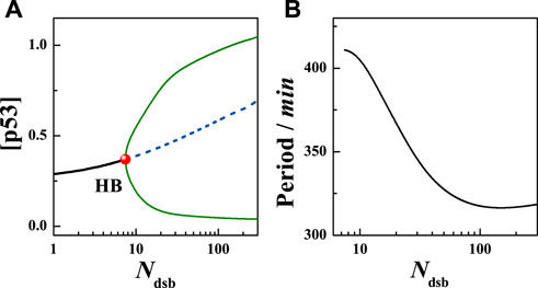
FIGURE 2. Deterministic analysis of the model. (A) The bifurcation diagram of total p53 concentration with N_dsb, the black solid line and dotted line represent stable and unstable states respectively, the solid circle represents the HB point, and the blue curve represents the maximum and minimum of [p53] in the limit cycle. (B) The change of [p53] with N_dsb. Here [p53] = [p53_u]+[p53_p].

FIGURE 3

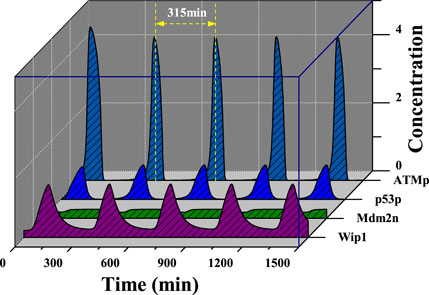
FIGURE 3. Time evolutions of [ATM_p], [p53_p], [Mdm2_n], [Wip1] with N_dsb = 175.

3.2 Bifurcation analysis of the negative feedback strength

The classical pathway for the negative regulation of p53 by Wip1 is the dephosphorylation of ATM at the Ser1981 site [18, 19], which corresponds to the parameter k_deatmwip. That is, the value of k_deatmwip affects the strength of the ATM-p53-Wip1 negative feedback loop. In order to explore the influence of this parameter on the network system, the value of k_deatmwip was changed independently. The results show that this parameter exerts great influence on the system state. For example, if k_deatmwip is taken as 0.05, 0.3 and 0.62 respectively, the state of the system variable changes significantly. As shown in the Figure 4, the time series of [p53_p] can show stable high level, periodic oscillation state and stable low level changes respectively. Here, the parameter N_dsb = 175.

FIGURE 4

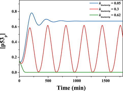
FIGURE 4. Time evolutions of [p53_p], with different k_deatmwip. From top to down, k_deatmwip = 0.05, 0.3, 0.62 respectively. The parameter N_dsb = 175.

Next, in order to obtain a more comprehensive understanding, the one-dimensional parameter bifurcation diagram of the system is calculated by changing the value of N_dsb. The calculation results show that the system state changes greatly with N_dsb. Regardless of the global solution in mathematics, the case of N_dsb > 0 is considered here. It is found that the system can present two forms of solutions: steady-state solution or oscillatory solution. Taking different values of k_deatmwip, the bifurcation diagram changes obviously, as shown in Figure 5. This shows the potential ability of parameter k_deatmwip in regulating cell state under different IR doses.

FIGURE 5

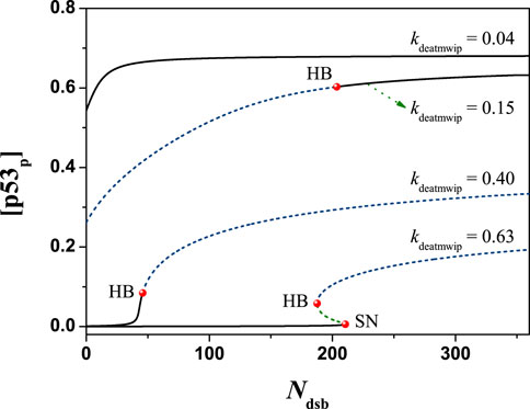
FIGURE 5. The bifurcation diagram of [p53_p] with N_dsb, the black solid line and dotted line represent stable and unstable states respectively, the symbol ‘HB’ represents the Hopf bifurcation point, and the symbol ‘SN’ represents the Saddle-Node bifurcation point. From top to down, k_deatmwip = 0.04, 0.15, 0.40, 0.63 respectively. The parameter N_dsb = 175.

Furthermore, the regulation of parameter k_deatmwip on the system state been focused. After numerical analysis, the equilibrium state of [p53_p] was obtained in relation to the variation of the parameter k_deatmwip, i.e., Figure 6. On the bifurcation diagram, three bifurcation points can be observed sequentially with increasing k_deatmwip: Hopf bifurcation point (HB), Saddle Node bifurcation point (SN) and Saddle Node Homoclinic bifurcation point (SNIC), same as the results in model [25]. The line between HB and SN is the unstable focus and saddle point, the line between SN and SNIC is the unstable saddle point, while the line outside HB and SNIC represents the stable point of the system. What is interesting is that a stable limit cycle can be found in the system, which is located between HB and SNIC, where stable periodic oscillations will occur. Here the [p53_p] concentrations changes differently. For example, when N_dsb = 175, the bifurcation diagram shows that the parameter k_deatmwip is in the (0, HB) interval and the negative feedback strength is relatively weak, [p53_p] is in the high state; the parameter k_deatmwip is in the (SNIC, + ∞) interval and the negative feedback strength is relatively high, [p53_p] is in the low steady state; the parameter k_deatmwip is in the (HB, SNIC) interval and the negative feedback strength is relatively weak [p53_p] is in the changeable steady state. The parameter k_deatmwip was in the (HB, SNIC) interval and produced stable non-decaying periodic oscillations. This indicates that Wip1-mediated negative feedback is important for p53 oscillations, which is consistent with the article [24]. Under different value of N_dsb, for instance N_dsb = 10, 35, 175, 350, the patterns of bifurcation diagrams vary greatly. This shows that k_deatmwip and N_dsb can affect the system together.

FIGURE 6

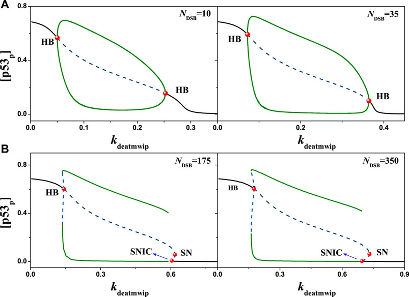
FIGURE 6. The bifurcation diagram of [p53_p] with k_deatmwip, the black solid line and dotted line represent stable and unstable states respectively, the symbol ‘HB’ represents the Hopf bifurcation point, the symbol ‘SN’ represents the Saddle-Node bifurcation point, and the symbol ‘SNIC’ represents the Saddle Node Homoclinic bifurcation point. (A) From left to right, N_dsb = 10 and 35 respectively. (B) From left to right, N_dsb = 175 and 350 respectively. Either in (A) or (B), the same ordinate system is used for the left and right graphs.

Here, the synergistic effect of positive and negative feedback is responsible for this change on the bifurcation diagram. When k_deatmwip is very small, the positive feedback effect on ATM will be quite strong, which can make ATM activated quickly. As the phosphorylation of p53 is mainly dominated by ATM, thus p53 can rise to a high level quickly, even N_dsb is quite small. So there is no oscillation. Next, when k_deatmwip increases, the positive feedback effect on ATM is weakened, and the negative feedback effect is strengthened, thus the periodic oscillation appears. The k_deatmwip value continues to rise, the positive feedback effect on ATM is weakened too, and the level of p53 rises slowly with N_dsb. As the oscillation needs a proper range of [p53_p], so the HB moves right at the N_dsb axis in Figure 5. If k_deatmwip value is very large, the positive feedback effect on ATM will be seriously weakened. So, given a quite large N_dsb value can ATM starts to activate and the periodic oscillation begins appear. Meanwhile, with the increasing N_dsb value, the equilibrium point of the system may changes from the stable node towards an unstable focus, thus evolving into the SNIC.

The changes of oscillation period can also be obtained with different parameters of k_deatmwip, which shows a same trend: first is rapid increasing, following with a flat platform and final is rapid increasing (seen in Figure 7). Without losing generality, we select a flat period region with up limit of 332.5 min, and determine the k_deatmwip region for oscillation, where a wide range can be seen for high N_dsb values. Especially, they are k_deatmwip = 0.445 and 0.5273 with N_dsb = 175 and 350 respectively. The flat period region means the period value can be observed in the experiment with high probability. For relevant cell experiments, that means a suitable negative feedback strength should be required for a realistic and stable oscillation period.

FIGURE 7

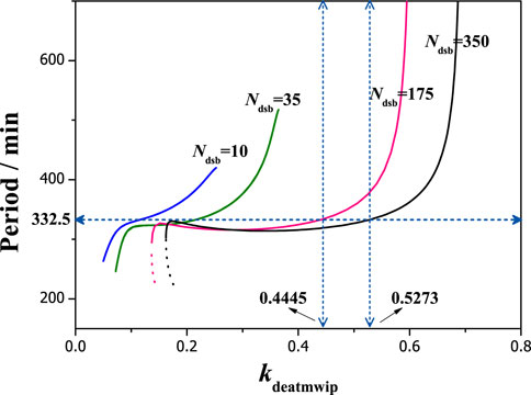
FIGURE 7. The dependence of period on the parameter k_deatmwip with different N_dsb. From left to right, N_dsb = 10, 35, 175, 350 respectively. The horizontal dots line denotes the period of 332.5 min. The vertical dots lines indicate k_deatmwip = 0.4445, 0.5273 respectively.

The above results were obtained only for N_dsb = 10, 35, 175, 350, but practical experiments [18] indicate that periodic oscillations of p53 can be detected when the iron-radiation dose exceeds a certain threshold, i.e., when the amount of DNA damage is greater than a certain value. A more complete understanding can be obtained by the distribution of network states on a two-dimensional parameter plane. Taking the k_deatmwip-N_dsb two-dimensional parameter space as an example, the relevant bifurcation curves were obtained in Figure 8. In this two-dimensional parameter space there are three states: stable steady state I, stable oscillatory state II and excitable state III. Among them, excitable state III can only be found if k_deatmwip and N_dsb are above a certain value (0.5246, 80). The results in Figure 8 also show that only if the strength of k_deatmwip is appropriate can stable p53 oscillation will appear. If k_deatmwip is too low or close to zero, there is no oscillatory state II, which is consistent with the experimental phenomenon in UV-irradiated cells [18], where the Wip1-ATM pathway is not activated. The results in Figure 8 may also provide some theoretical explanation for the experiments of Chen et al [35]. Namely that the strength of k_deatmwip in cells is in a specific range and that p53 oscillations can only occur when the dose of etoposide (amount of DNA damage) is moderate.

FIGURE 8

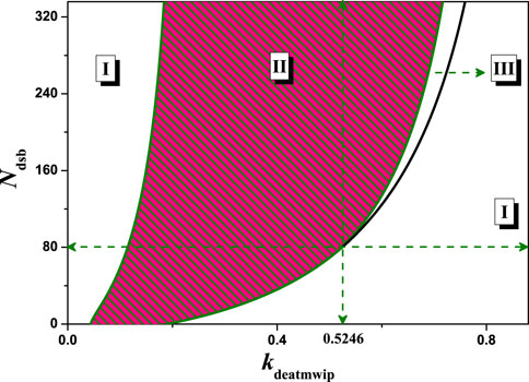
FIGURE 8. The two-parameter bifurcation with respect to k_deatmwip and N_dsb. The symbols ‘I’,‘II’ and ‘III’ represent monostable state, oscillation state and excited state respectively. The vertical dots line indicates k_deatmwip = 0.5246.

3.3 Self-antagonism of the ATM-p53-Wip1 NFL

The above results mainly reflect the situation in the ATM-p53-Wip1 negative feedback loop after changing the strength of a single feedback. In the actual cellular setting, there may be other antagonistic effects in the same loop that are worth considering. For example, in this model the dephosphorylation of Ser1981 by Wip1 on ATM and the phosphorylation of Ser15 by ATM on p53 [41]. In this model, the parameter k_acp531 is used to represent the strength of ATM phosphorylation on p53. Numerical analysis yielded the equilibrium state of [p53_p] in relation to the parameter k_deatmwip, i.e., in Figure 9. When k_acp531 = 0.08, with N_dsb = 175 the bifurcation diagrams are consistent with Figure 6. But, when k_acp531 = 0.2, only two Hopf bifurcation points can be observed as k_deatmwip increases, indicating a sudden change in the equilibrium state of the system. As the parameter k_deatmwip increases, the period exerts the same tends as in Figure 7 when N_dsb = 175.

FIGURE 9

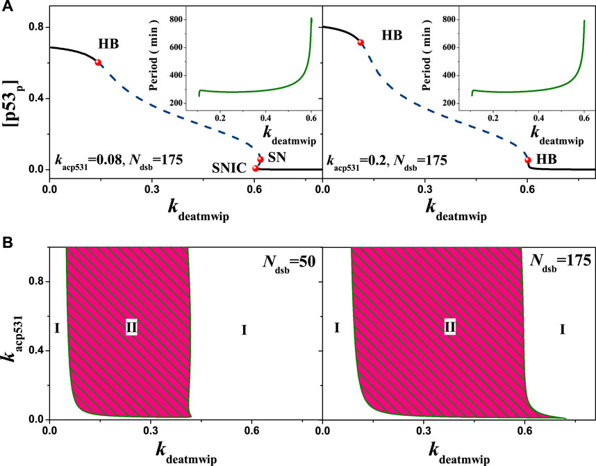
FIGURE 9. Influences of the ATM regulated p53 phosphorylation on the network dynamics with different strengths. (A) One parameter bifurcation diagram of [p53_p] on the parameter k_deatmwip. From left to right, k_acp531 = 0.08 and 0.20 respectively. The schematic diagram shows the relationship between the period and the parameters k_deatmwip. (B) The two-parameter bifurcation with respect to k_deatmwip and k_acp531. The symbols ‘I’, ‘II’ and ‘III’ represent monostable state, oscillation state and excited state respectively. From left to right, N_dsb = 50 and 175 respectively. Either in A or B, the same ordinate system is used for the left and right graphs.

The above changes can be interpreted from the relevant dynamics in detail. When the parameter k_deatmwip is in the range (0,HB), indicating relative low negative feedback strength, which may benefit the high level of p53 phosphorylation, thus there is only stable equilibrium state. On contrary, when k_deatmwip is in the range (SNIC, +∞) (k_acp531 = 0.08) or the range (HB, +∞) (k_acp531 = 0.2), the p53 phosphorylation will be suppressed, the system will also go to stable equilibrium state. Only when k_deatmwip is in the range (HB, SNIC) or (HB, HB), the stable oscillation can appears. This may indicate the importance of the appropriate feedback strength for p53 oscillation. And the emergence of SNIC when k_acp531 = 0.08 suggests that the antagonism increases the complexity of the same feedback loop. When k_acp531 = 0.2, the k_deatmwip range for p53 oscillation becomes larger, suggesting that the increased phosphorylation on p53 at Ser15 may contribute to the arise of stable oscillatory states. It is worth nothing to mention that, due to the nonlinear synergistic effect, with a higher phosphorylation strength on p53, the a stable limit loop will surround an unstable focus instead of unstable node, which causes the change from SNIC to HB, as in Figure 9A.

Furthermore, a more clear understanding can be obtained by two-dimensional bifurcation diagram. Within different DNA damage, the k_deatmwip-k_acp531 bifurcation diagram can be obtained by extending each bifurcation point, i.e., Figure 9B. For N_dsb = 50, the system oscillation state II corresponds to a smaller value of k_deatmwip and a larger range of k_acp531 values, indicating that the amount of Ser15 phosphorylation of p53 is important, i.e., a stable periodic oscillation can also be maintained by weak Ser15 phosphorylation of p53. At N_dsb = 175, the parameter range of systemic oscillation state II was relatively broadened, indicating a high correlation between the amount of DNA damage and the stable oscillation state. Comparing the above results, a more plausible explanation is that DNA damage acts directly on ATM, and ATM can phosphorylate p53, as DNA damage amplifies the signal through positive feedback from ATM, which facilitating the emergence of oscillations, in consist with the findings in the study [25, 31, 32, 42]. These founds also indicate the need of coordinated mutual antagonism in the same feedback loop in order to maintain stable periodic oscillations.

3.4 Synergies of coupled PFL and NFL

Different from the above discussion in the same feedback loop, we further analyzed a pair of opposite effect on the same protein, e.g., the phosphorylation and dephosphorylation on ATM. In this model, the ATM autophosphorylation is considered, different from the phosphorylation of Mdm2 at Ser395 [25], as in research it is confirmed that ATM autophosphorylation happens more often, which can accelerate the ATM activation to a higher level quickly [36], forming a PFL. To test whether DNA damage amplifies the signal through ATM’s PFL more conducive to oscillations, we make a test by comparison. Generally, in coupled PFL and NFL, oscillation is dominated by NFL, and PFL exerts a gain effect on NFL [32]. In this model, p53-Wip1-ATM and p53-Mdm2 NFLs coexist. Numerical analysis shows that the value range of the oscillation parameter k_deatmwip of the system becomes wider by increasing of the positive feedback strength parameter k_acatm, as shown in Figure 10. Although the value of k_acatm is zero representing no phosphorylation on p53, the oscillation range can also be found with proper k_deatmwip values, indicating that the oscillation is dominated by p53-Mdm2 loop. In the two-parameter bifurcation diagram, the oscillable k_deatmwip interval widens with the increase of k_acatm, indicating that the increase of positive feedback amplifies the signal and is conducive to p53 oscillation.

FIGURE 10

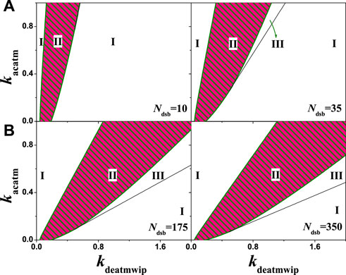
FIGURE 10. The two-parameter bifurcation with respect to k_deatmwip and k_acatm. The symbols ‘I’,‘II’, and ‘III’ represent monostable state, oscillation state and excited state respectively. (A) From left to right, N_dsb = 10,35 respectively. (B) From left to right, N_dsb = 175, 350 respectively. Either in A or B, the same ordinate system is used for the left and right graphs.

The more damage, the more oscillating region will appear in the system, as well as the excitable state III. The possible reason is that DNA damage directly acts on substrate ATM, which changes the positive feedback intensity of ATM. The change of positive feedback strength leads to the change of equilibrium property of the system, causing the change of system state. That means the positive feedback increases the complexity of system state. Since the appearance of the oscillating state requires a specific range of positive and negative feedback intensity, it also indicates that the oscillation is the result of the coordination of positive and negative feedback. General research models also confirm [31, 32, 42] that the network model coupled with PFLs and NFLs has better robustness and better response in the p53 network.

3.5 Bottleneck like effect of p53-Wip1-ATM and p53-Mdm2 NFLs

Further, in addition to the coupled PFL and NFL in a single loop discussed above, there are also coupled NFLs in this system, deserving much attentions. For example, the negative feedback collaboration between p53-Wip1-ATM and p53-Mdm2. Here, we first paid special attention to the degradation of intranuclear Mdm2 regulated by phosphorylated ATM, which essentially constitutes a nested ATM-Mdm2-p53-Wip1 NFL that partially overlaps with the pathway of the p53-Wip1-ATM and p53-Mdm2 NFL. In contrast to the previous use of the Mdm2 inhibitor Nutlin-3 to activate the p53 signaling pathway [43], here, regulating the coupled NFLs to achieve state transition can be a new try. In this model, the strength of Mdm_n degradation by ATM is reflected in the key parameter k_dmdm2n1. Within different conditions, the 1-D bifurcation diagrams of k_dmdm2n1 can be obtained. As shown in Figure 11A, the parameter range of the scalable k_dmdm2n1 was found to change significantly after fixing the intensity of dephosphorylation of ATM by Wip1, and the corresponding oscillation period varied in the same trend with k_dmdm2n1. The scalable k_dmdm2n1 range was larger for smaller values of k_deatmwip (k_deatmwip = 0.15) and smaller for larger k_deatmwip (k_deatmwip = 0.24), indicating their mutually exclusive nature. Thus, the competitive involution may cause the limitation of oscillation, showing a bottleneck like effect on N_dsb. In the k_deatmwip-k_dmdm2n1 two dimensional bifurcation diagrams, this effect was very obvious. For different N_dsb, e.g., N_dsb = 50 and 175 respectively, oscillation regions tending to be concave towards the origin, as in Figure 11B. This change in the oscillable parameter region reflects the competing effects of the two NFLs. The scalable parameter region is different, indicating that the amount of DNA damage dominates the neck of p53 oscillation.

FIGURE 11

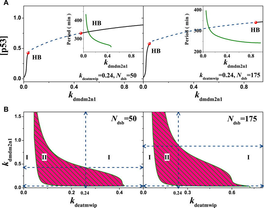
FIGURE 11. Influences of the ATM regulated Mdm2n degradation on the network dynamics with different strengths. (A) One parameter bifurcation diagram of [p53] on the parameter k_dmdm2n1. From left to right, k_deatmwip = 0.15 and 0.24 respectively. The schematic diagram shows the relationship between the period and the parameters k_dmdm2n1. (B) The two-parameter bifurcation with respect to k_deatmwip and k_dmdm2n1. The symbols ‘I’,‘II’ and ‘III’ represent monostable state, oscillation state and excited state respectively. From left to right, N_dsb = 50 amd 175 respectively. Either in A or B, the same ordinate system is used for the left and right graphs.

This bottleneck like effect is most likely due to the fact that ATM-promoted degradation of Mdm2, in which larger values of k_dmdm2n1 implying higher levels of p53, when the system is prone to oscillation or instability. The higher dephosphorylation on ATM tends to disrupt the equilibrium, thus lowering the p53 expression and making the system monostable, also the lower dephosphorylation intensity on ATM tends to raise the p53 expression and make the system tends to the other extreme. Only when the two are coordinated can stable oscillations be generated. For N_dsb = 50, the oscillatory region in the two dimensional bifurcation diagram has no intersection with either axis, indicating that the p53-Mdm2 pathway and the p53-Wip1-ATM pathway are equally important for oscillations. So, this nested coupling of the dual NFls constrains each other and creates a competitive effect, limiting the scale of the parameters region.

3.6 Theoretical analysis

In this subsection, we further conduct a theoretical analysis on the above results, aim at revealing the underlying physical mechanism. As far as we know, such feedback loops as coupled PFL and NFL have been widely studied in the literature. Here, we are more concerned with the special pathway of coupled NFLs. By simplifying the biochemical reaction process between different proteins, we obtained the abstract structural diagram of p53 core network, as shown in Figure 12.

FIGURE 12

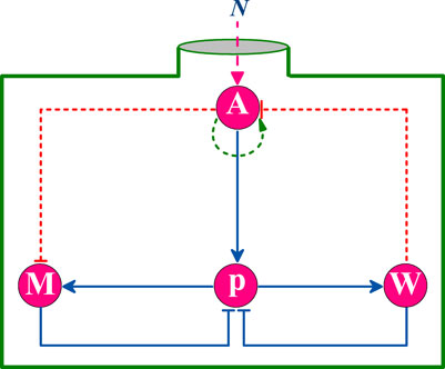
FIGURE 12. Simplified system network structure diagram. N represents the DNA damage number.

For such a simplified network model, we can infer that its responding capacity for stress signals depends on the short board in the signaling pathway, e.g., the node with the weakest interaction ability, reflecting as the bottleneck effect on strength. Assuming that each node protein in the network can equally participate in the reaction, the core node protein, as the busiest one, is easier to become a short board. In this coupled NFLs model, considering the reaction process that p53 actually participates in, we introduced anti-competitive inhibition dynamics to analogize the related dynamics. The mechanism of anti-competitive inhibition can be expressed as,

$\mathrm{W}+\mathrm{P}\stackrel{k_{+1}}{\underset{k_{-1}}{\rightleftharpoons }}\left[\mathrm{W}\mathrm{P}\right]\stackrel{k_{+2}}{\to }\mathrm{W}+{\mathrm{P}}^{\prime }$

$\left[\mathrm{W}\mathrm{P}\right]+\mathrm{M}\stackrel{k_{+3}}{\underset{k_{-3}}{\rightleftharpoons }}\left[\mathrm{W}\mathrm{M}\mathrm{P}\right]$

where, W,P and M can represents Wip1, p53 and Mdm2 respectively.

Based on the steady-state assumption, the following equations can be listed:

$\frac{d[\mathrm{W}\mathrm{P}]}{\mathrm{d}t}=k_{+1}\left[\mathrm{W}\right]\left[\mathrm{P}\right]-\left(k_{-1}+k_{+2}\right)\left[\mathrm{W}\mathrm{P}\right]=0,(11)$

$\frac{d[\mathrm{W}\mathrm{M}\mathrm{P}]}{\mathrm{d}t}=k_{+3}\left[\mathrm{W}\mathrm{P}\right]\left[\mathrm{M}\right]-\left(k_{-3}\right)\left[\mathrm{W}\mathrm{M}\mathrm{P}\right]=0,(12)$

$\left[{\mathrm{W}}_{\text{0}}\right]=\left[\mathrm{W}\right]+\left[\mathrm{W}\mathrm{P}\right]+\left[\mathrm{W}\mathrm{M}\mathrm{P}\right],(13)$

$r_{\text{WP}}=k_{+2}\left[\mathrm{W}\mathrm{P}\right],(14)$

After integration, one can get

$r_{\text{WP}}=\frac{r_{\text{max}}\left[\mathrm{P}\right]}{K_{\text{m}}+\left[\mathrm{P}\right]+\left[\mathrm{P}\right]\left[\mathrm{M}\right]/K_{\text{M}}}=\frac{r_{\text{max}}^{*}\left[\mathrm{P}\right]}{K_{\text{m}}^{*}+\left[\mathrm{P}\right]},(15)$

where,

$K_{\text{m}}^{*}=\frac{K_{\text{m}}}{1+\left[\mathrm{M}\right]/K_{\text{M}}},r_{\text{max}}^{*}=\frac{r_{\text{max}}}{1+\left[\mathrm{M}\right]/K_{\text{M}}}.(16)$

Here, $K_{\text{m}}^{*}$ is the apparent Michaelis constant in the presence of inhibitors, K_M is the dissociation constant of inhibitor, r_max is the maximum initial rate without inhibitor, and K_m is the apparent Michaelis constant without inhibitors. It can be seen from the Eq. 15 that when [M] increases or K_M decreases, $K_{\text{m}}^{*}$ will increase, thereby inhibiting the decline of substrate P reaction rate. The relationship between reaction rate r_PM and substrate concentration P is shown in Figure 13. It can be seen that with the increasing substrate concentration [P], the degree of competitive inhibition will decrease, but it will gradually show a saturated state.

FIGURE 13

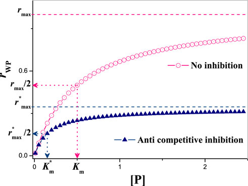
FIGURE 13. The dependence of r_PM on [P] under anti-competitive inhibition. Without losing generality, K_m = 0.5, r_max = 1.0, K_M = 0.5 and [M] = 1.0. So, $K_{\text{m}}^{*}=0.167$, $r_{\text{max}}^{*}=0.333$.

In order to reflect the inhibition degree of the inhibitor on the reaction, we define a physical quantity: i,

$i=\frac{r_{\text{P}}-r_{\text{PM}}}{r_{\text{P}}}\cdot 100\%,(17)$

where, r_P = r_max [P]/(K_m + [P]) is the production rate of P′ without inhibitor.

For this model, it has

$i=\frac{\left[\mathrm{P}\right]\left[\mathrm{M}\right]}{K_{\text{M}}\left(\left[\mathrm{P}\right]+K_{\text{m}}\right)+[\mathrm{P}][\mathrm{M}]}\cdot 100\%.(18)$

So, from the Eq. 18 it can be inferred that the inhibition degree of inhibitors can be reduced by increasing [P] and the competitive oscillations can be mitigated. But increasing [P] can only alleviate the inhibition in a certain range. As, given larger [P] the oscillation will be destroyed. Through comparison, it can be seen that without the inhibitor [M], the NFL of AMT-p53-Wip1 can run well, e.g., the oscillation of a single negative feedback loop network seems to have more control advantages, but the disadvantages are also obvious: poor robustness. Therefore, we suggest that adding multiple positive feedback pathways to this p53 network may be a better choice.

4 Discussion

Classical theories suggest that multiple NFLs in the cell network combined with time delays in such process as gene transcription, protein translation and protein entry or exit from the nucleus, are the main causes of oscillations in the p53 protein network [21]. And it also demonstrated that positive feedback regulates the gain of negative feedback, which can be used to regulate this present model. In contrast to the positive feedback between p53 and Mdm2 mentioned in the article [25], the positive feedback in this model comes from the phosphorylation of ATM. The positive feedback of ATM up-regulates the p53-Mdm2 negative feedback loop, thus facilitating the threshold effect on the amount of DNA damage. The coupled positive-negative or negative-negative feedback enriches the kinetic behavior of the p53 protein network. What’s more, the bottleneck effect caused by coupled NFLs firstly proposed by us in this model is still deserves further attention. Whether this effect only appears in p53 network or in other networks needs further confirmation. It is undeniable that the appearance of this coupled NFLs motif limits the overall response range, and new methods need to be considered for improvement, as it is still an effective way in clinical medicine to achieve tumor inhibition by regulating p53 network and related components [44, 45]. In any case, the understanding from the details of this model can be more generalizable for other network models with feedback loops. In addition, it is worth nothing that the system of ordinary differential equations and the Hill function in the deterministic model can only characterize the statistical behaviour of proteins in subcellular levels. To achieve more, molecular-level modelling is required, as well as the corresponding molecular dynamics methods. What’s more, from an abstract perspective, p53 network consists of nodes, edges, and typical topological motifs, which can form a small scale-free network. Stimulated by the external signals, the self-dynamics and interaction dynamics of p53 network will change accordingly, reflecting the adaptability of cells. Understanding the spatiotemporal signal propagation [46–48] in this network with perturbations ideas may bring some inspiration.

5 Conclusion

In summary, this paper focuses on the dephosphorylation of ATM by Wip1 and discusses the this modification process on ATM, p53 and Mdm2, as well as the p53 oscillation phenomenon in detail. After constructing a mathematical model of the p53 protein network in accordance with the classical understanding, we investigated the regulation of p53 network oscillations by Wip1 dephosphorylation on ATM using the ordinary differential equations as the main concern for parametric bifurcation analysis. The results showed that: 1) the Wip1-ATM-p53 loop, where Wip1 dephosphorylation and p53 phosphorylation can form an internal mutual antagonism, is necessary to maintain stable limit cycle oscillations. And the different intensity of Wip1 dephosphorylation can provide a partial explanation for the response of p53 protein under UV or IR radiation; 2) the PFL of ATM autophosphorylation is coupled with the Wip1-ATM-p53 NFL, which can increase the gain of the NFL [32], ensuring robust oscillations; 3) the p53-Wip1-ATM loop and the p53-Mdm2 loop can form a coupled double NFL, which resists each other and suppresses the expansion of the oscillable parameter region, creating an Bottleneck-like effect. In order to alleviate this constraint, we suggest adding a positive feedback signal pathway to achieve better oscillation stability. Overall, this paper shows that either antagonism of the same loop or coupling of different loops can regulate the p53 network, and that periodic oscillations are the result of the coordination of various strengths in the structure of the coupled network. This conclusion has implications for other network models where oscillations occur. In addition, the downstream related genes and proteins of the p53 protein network are closely related to cell cycle, apoptosis and cellular senescence [13], is worth further analysis. It is also hoped that the results of this study will provide a useful reference for researches on related cellular diseases.

Data availability statement

The original contributions presented in the study are included in the article/supplementary material, further inquiries can be directed to the corresponding author.

Author contributions

DW and ZW completed the result analysis and wrote the first draft of the manuscript. YW and XL participated in manuscript design and results analysis. DW and HL contributed to conception and design of the study. DW, HL, and XL was responsible for manuscript writing and revision. All authors contributed to manuscript revision, read, and approved the submitted version.

Funding

This work was supported by the National Natural Science Foundation of China (Grant Nos. 11804123 and 12175087) and the special program of the National Natural Science Foundation of China (Grant No. 11547025).

Acknowledgments

We sincerely thank all the reviewers, editors, and frontiers editorial staff for their constructive advices and excellent work.

Conflict of interest

The authors declare that the research was conducted in the absence of any commercial or financial relationships that could be construed as a potential conflict of interest.

Publisher’s note

All claims expressed in this article are solely those of the authors and do not necessarily represent those of their affiliated organizations, or those of the publisher, the editors and the reviewers. Any product that may be evaluated in this article, or claim that may be made by its manufacturer, is not guaranteed or endorsed by the publisher.

References

1. Vogelstein B, Lane D, Levine AJ. Surfing the p53 network. Nature (2000) 408:307–10. doi:10.1038/35042675

PubMed Abstract | CrossRef Full Text | Google Scholar

2. Linzer DI, Levine AJ. Characterization of a 54k Dalton cellular sv40 tumor antigen present in sv40-transformed cells and uninfected embryonal carcinoma cells. Cell (1979) 17:43–52. doi:10.1016/0092-8674(79)90293-9

PubMed Abstract | CrossRef Full Text | Google Scholar

3. Levine AJ. p53: 800 million years of evolution and 40 years of discovery. Nat Rev Cancer (2020) 20:471–80. doi:10.1038/s41568-020-0262-1

PubMed Abstract | CrossRef Full Text | Google Scholar

4. Vousden KH, Lane DP. p53 in health and disease. Nat Rev Mol Cel Biol (2007) 8:275–83. doi:10.1038/nrm2147

PubMed Abstract | CrossRef Full Text | Google Scholar

5. Jackson SP, Bartek J. The dna-damage response in human biology and disease. Nature (2009) 461:1071–8. doi:10.1038/nature08467

PubMed Abstract | CrossRef Full Text | Google Scholar

6. Che Z, Sun H, Yao W, Lu B, Han Q. Role of post-translational modifications in regulation of tumor suppressor p53 function. Front Oral Maxillofac Med (2020) 2:1–11. doi:10.21037/fomm.2019.12.02

CrossRef Full Text | Google Scholar

7. Kubbutat MH, Jones SN, Vousden KH. Regulation of p53 stability by mdm2. Nature (1997) 387:299–303. doi:10.1038/387299a0

PubMed Abstract | CrossRef Full Text | Google Scholar

8. Guo L, Liew H, Camus S, Goh A, Chee L, Lunny D, et al. Ionizing radiation induces a dramatic persistence of p53 protein accumulation and dna damage signaling in mutant p53 zebrafish. Oncogene (2013) 32:4009–16. doi:10.1038/onc.2012.409

PubMed Abstract | CrossRef Full Text | Google Scholar

9. Kahlert C, Melo SA, Protopopov A, Tang J, Seth S, Koch M, et al. Identification of double-stranded genomic dna spanning all chromosomes with mutated kras and p53 dna in the serum exosomes of patients with pancreatic cancer. J Biol Chem (2014) 289:3869–75. doi:10.1074/jbc.C113.532267

PubMed Abstract | CrossRef Full Text | Google Scholar

10. Berkers CR, Maddocks OD, Cheung EC, Mor I, Vousden KH. Metabolic regulation by p53 family members. Cell Metab (2013) 18:617–33. doi:10.1016/j.cmet.2013.06.019

PubMed Abstract | CrossRef Full Text | Google Scholar

11. Maddocks OD, Berkers CR, Mason SM, Zheng L, Blyth K, Gottlieb E, et al. Serine starvation induces stress and p53-dependent metabolic remodelling in cancer cells. Nature (2013) 493:542–6. doi:10.1038/nature11743

PubMed Abstract | CrossRef Full Text | Google Scholar

12. Shaltiel IA, Aprelia M, Saurin AT, Chowdhury D, Kops GJ, Voest EE, et al. Distinct phosphatases antagonize the p53 response in different phases of the cell cycle. Proc Natl Acad Sci U S A (2014) 111:7313–8. doi:10.1073/pnas.1322021111

PubMed Abstract | CrossRef Full Text | Google Scholar

13. Garcia-Barros M, Paris F, Cordon-Cardo C, Lyden D, Rafii S, Haimovitz-Friedman A, et al. Tumor response to radiotherapy regulated by endothelial cell apoptosis. Science (2003) 300:1155–9. doi:10.1126/science.1082504

PubMed Abstract | CrossRef Full Text | Google Scholar

14. Hafner A, Bulyk ML, Jambhekar A, Lahav G. The multiple mechanisms that regulate p53 activity and cell fate. Nat Rev Mol Cel Biol (2019) 20:199–210. doi:10.1038/s41580-019-0110-x

PubMed Abstract | CrossRef Full Text | Google Scholar

15. Zhang XP, Liu F, Cheng Z, Wang W. Cell fate decision mediated by p53 pulses. Proc Natl Acad Sci U S A (2009) 106:12245–50. doi:10.1073/pnas.0813088106

PubMed Abstract | CrossRef Full Text | Google Scholar

16. Zhang XP, Liu F, Wang W. Two-phase dynamics of p53 in the dna damage response. Proc Natl Acad Sci U S A (2011) 108:8990–5. doi:10.1073/pnas.1100600108

PubMed Abstract | CrossRef Full Text | Google Scholar

17. Purvis JE, Karhohs KW, Mock C, Batchelor E, Loewer A, Lahav G. p53 dynamics control cell fate. Science (2012) 336:1440–4. doi:10.1126/science.1218351

PubMed Abstract | CrossRef Full Text | Google Scholar

18. Batchelor E, Mock CS, Bhan I, Loewer A, Lahav G. Recurrent initiation: A mechanism for triggering p53 pulses in response to dna damage. Mol Cel (2008) 30:277–89. doi:10.1016/j.molcel.2008.03.016

PubMed Abstract | CrossRef Full Text | Google Scholar

19. Shreeram S, Demidov ON, Hee WK, Yamaguchi H, Onishi N, Kek C, et al. Wip1 phosphatase modulates atm-dependent signaling pathways. Mol Cel (2006) 23:757–64. doi:10.1016/j.molcel.2006.07.010

PubMed Abstract | CrossRef Full Text | Google Scholar

20. Bakkenist CJ, Kastan MB. Dna damage activates atm through intermolecular autophosphorylation and dimer dissociation. Nature (2003) 421:499–506. doi:10.1038/nature01368

PubMed Abstract | CrossRef Full Text | Google Scholar

21. Lev Bar-Or R, Maya R, Segel LA, Alon U, Levine AJ, Oren M. Generation of oscillations by the p53-mdm2 feedback loop: A theoretical and experimental study. Proc Natl Acad Sci U S A (2000) 97:11250–5. doi:10.1073/pnas.210171597

PubMed Abstract | CrossRef Full Text | Google Scholar

22. Lahav G, Rosenfeld N, Sigal A, Geva-Zatorsky N, Levine AJ, Elowitz MB, et al. Dynamics of the p53-mdm2 feedback loop in individual cells. Nat Genet (2004) 36:147–50. doi:10.1038/ng1293

PubMed Abstract | CrossRef Full Text | Google Scholar

23. Geva-Zatorsky N, Rosenfeld N, Itzkovitz S, Milo R, Sigal A, Dekel E, et al. Oscillations and variability in the p53 system. Mol Syst Biol (2006) 2:2006.0033. doi:10.1038/msb4100068

PubMed Abstract | CrossRef Full Text | Google Scholar

24. Wang DG, Zhou CH, Zhang XP. The birhythmicity increases the diversity of p53 oscillation induced by dna damage. Chin Phys B (2017) 26:128709. doi:10.1088/1674-1056/26/12/128709

CrossRef Full Text | Google Scholar

25. Yang HL, Liu N, Yang LG. Influence of mdm2-mediated positive feedback loop on the oscillation behavior of p53 gene network. Acta Phys Sin (2021) 70(13):138701–9. doi:10.7498/aps.70.20210015

CrossRef Full Text | Google Scholar

26. Ouattara DA, Abou-Jaoudé W, Kaufman M. From structure to dynamics: Frequency tuning in the p53-mdm2 network. ii: Differential and stochastic approaches. J Theor Biol (2010) 264:1177–89. doi:10.1016/j.jtbi.2010.03.031

PubMed Abstract | CrossRef Full Text | Google Scholar

27. Ma L, Wagner J, Rice JJ, Hu W, Levine AJ, Stolovitzky GA. A plausible model for the digital response of p53 to dna damage. Proc Natl Acad Sci U S A (2005) 102:14266–71. doi:10.1073/pnas.0501352102

PubMed Abstract | CrossRef Full Text | Google Scholar

28. Jun-Feng X, Ya J. A mathematical model of a p53 oscillation network triggered by dna damage. Chin Phys B (2010) 19:040506. doi:10.1088/1674-1056/19/4/040506

CrossRef Full Text | Google Scholar

29. Wang DG, Wang S, Huang B, Liu F. Roles of cellular heterogeneity, intrinsic and extrinsic noise in variability of p53 oscillation. Sci Rep (2019) 9:5883. doi:10.1038/s41598-019-41904-9

PubMed Abstract | CrossRef Full Text | Google Scholar

30. Wang YL, Liu F. Transcription apparatus: A dancer on a rope. Acta Phys Sin (2020) 69:248702. doi:10.7498/aps.69.20201631

CrossRef Full Text | Google Scholar

31. Wang LS, Li NX, Chen JJ, Zhang XP, Liu F, Wang W. Modulation of dynamic modes by interplay between positive and negative feedback loops in gene regulatory networks. Phys Rev E (2018) 97:042412. doi:10.1103/PhysRevE.97.042412

PubMed Abstract | CrossRef Full Text | Google Scholar

32. Huang B, Tian X, Liu F, Wang W. Impact of time delays on oscillatory dynamics of interlinked positive and negative feedback loops. Phys Rev E (2016) 94:052413. doi:10.1103/PhysRevE.94.052413

PubMed Abstract | CrossRef Full Text | Google Scholar

33. Li X, Liu F, Shuai JW. Dynamical studies of cellular signaling networks in cancers. Acta Phys Sin (2016) 65:178704. doi:10.7498/aps.65.178704

CrossRef Full Text | Google Scholar

34. Li X, Li Z, Yang W, Wu Z, Wang J. Bidirectionally regulating gamma oscillations in wilson-cowan model by self-feedback loops: A computational study. Front Syst Neurosci (2022) 16:723237–13. doi:10.3389/fnsys.2022.723237

PubMed Abstract | CrossRef Full Text | Google Scholar

35. Chen X, Chen J, Gan S, Guan H, Zhou Y, Ouyang Q, et al. Dna damage strength modulates a bimodal switch of p53 dynamics for cell-fate control. BMC Biol (2013) 11:73–11. doi:10.1186/1741-7007-11-73

PubMed Abstract | CrossRef Full Text | Google Scholar

36. Kozlov SV, Graham ME, Jakob B, Tobias F, Kijas AW, Tanuji M, et al. Autophosphorylation and atm activation: Additional sites add to the complexity. J Biol Chem (2011) 286:9107–19. doi:10.1074/jbc.M110.204065

PubMed Abstract | CrossRef Full Text | Google Scholar

37. Shiloh Y, Ziv Y. The atm protein kinase: Regulating the cellular response to genotoxic stress, and more. Nat Rev Mol Cel Biol (2013) 14:197–210. doi:10.1038/nrm3546

PubMed Abstract | CrossRef Full Text | Google Scholar

38. Wang HY, Zhang XP, Wang W. Regulation of epithelial-to-mesenchymal transition in hypoxia by the hif-1α network. FEBS Lett (2022) 596:338–49. doi:10.1002/1873-3468.14258

PubMed Abstract | CrossRef Full Text | Google Scholar

39. Dhooge A, Govaerts W, Kuznetsov YA. Matcont: A matlab package for numerical bifurcation analysis of odes. ACM Trans Math Softw (2003) 29:141–64. doi:10.1145/779359.779362

CrossRef Full Text | Google Scholar

40. Zingg DW, Chisholm TT. Runge–Kutta methods for linear ordinary differential equations. Appl Numer Math (1999) 31:227–38. doi:10.1016/S0168-9274(98)00129-9

CrossRef Full Text | Google Scholar

41. Thanasoula M, Escandell JM, Suwaki N, Tarsounas M. Atm/atr checkpoint activation downregulates cdc25c to prevent mitotic entry with uncapped telomeres. EMBO J (2012) 31:3398–410. doi:10.1038/emboj.2012.191

PubMed Abstract | CrossRef Full Text | Google Scholar

42. Zhang T, Brazhnik P, Tyson JJ. Exploring mechanisms of the dna-damage response: p53 pulses and their possible relevance to apoptosis. Cell Cycle (2007) 6:85–94. doi:10.4161/cc.6.1.3705

PubMed Abstract | CrossRef Full Text | Google Scholar

43. Christian T, James R, Zoran F, Brian H, Kenneth K, Holly H, et al. Small-molecule mdm2 antagonists reveal aberrant p53 signaling in cancer: Implications for therapy. Proc Natl Acad Sci U S A (2006) 103:1888–93. doi:10.1073/pnas.0507493103

PubMed Abstract | CrossRef Full Text | Google Scholar

44. Suarez OJ, Vega CJ, Sanchez EN, González-Santiago AE, Rodríguez-Jorge O, Alanis AY, et al. Pinning control for the p53-mdm2 network dynamics regulated by p14arf. Front Physiol (2020) 11:976. doi:10.3389/fphys.2020.00976

PubMed Abstract | CrossRef Full Text | Google Scholar

45. Duffy MJ, Synnott NC, Grady SÓ, Crown J. Targeting p53 for the treatment of cancer. Semin Cancer Biol (2022) 79:58–67. doi:10.1016/j.semcancer.2020.07.005

PubMed Abstract | CrossRef Full Text | Google Scholar

46. Hens C, Harush U, Haber S, Cohen R, Barzel B. Spatiotemporal signal propagation in complex networks. Nat Phys (2019) 15:403–12. doi:10.1038/s41567-018-0409-0

CrossRef Full Text | Google Scholar

47. Bao X, Hu Q, Ji P, Lin W, Kurths J, Nagler J. Impact of basic network motifs on the collective response to perturbations. Nat Commun (2022) 13:5301–8. doi:10.1038/s41467-022-32913-w

PubMed Abstract | CrossRef Full Text | Google Scholar

48. Ji P, Lin W, Kurths J. Asymptotic scaling describing signal propagation in complex networks. Nat Phys (2020) 16:1082–3. doi:10.1038/s41567-020-1025-3

CrossRef Full Text | Google Scholar