Network structure indexes to forecast epidemic spreading in real-world complex networks

Complex networks are the preferential framework to model spreading dynamics in several real-world complex systems. Complex networks can describe the contacts between infectious individuals, responsible for disease spreading in real-world systems. Understanding how the network structure affects an epidemic outbreak is therefore of great importance to evaluate the vulnerability of a network and optimize disease control. Here we argue that the best network structure indexes (NSIs) to predict the disease spreading extent in real-world networks are based on the notion of network node distance rather than on network connectivity as commonly believed. We numerically simulated, via a type-SIR model, epidemic outbreaks spreading on 50 real-world networks. We then tested which NSIs, among 40, could a priori better predict the disease fate. We found that the “average normalized node closeness” and the “average node distance” are the best predictors of the initial spreading pace, whereas indexes of “topological complexity” of the network, are the best predictors of both the value of the epidemic peak and the final extent of the spreading. Furthermore, most of the commonly used NSIs are not reliable predictors of the disease spreading extent in real-world networks.

Introduction

The fundamental role of networks in epidemiology has been recognized in the last years [1–12]. The disease spreading can be modeled as a network where nodes (vertices) represent the individuals (i.e., the hosts) and links (edges) indicate the social contacts among them [1–9]. Real-world complex networks display many structural connectivity patterns, such as the heavy-tailed degree distribution, small-world effect, high clustering coefficient, self-similarity, assortativity, community structures, etc. [1, 13–18]. These network structural connectivity patterns may affect the evolution of the spreading process [1, 5, 18–21]. Knowing the relationship between network structure indexes (NSIs) and the spreading dynamics is crucial to prevent and control diseases [17].

The field measures and analyses of real-world complex networks can be extremely consuming, in terms of both money and time. It is therefore necessary to know which features of the network structure should be first measured to assess the network vulnerability to disease and consequently optimize the control [1, 18–21]. To address this issue, we gathered a dataset of 50 real-world complex systems. They represent archetypical examples of network structures in different domains of reality, ranging from social, computers, internet, transportation, biological, and ecological networks (see Supplementary Materials S1.2 for details). We explicitly simulated a disease spreading over them via a classical compartmental susceptible–infected–recovered (SIR) model [1–5].

We derived three indicators of the speed and magnitude of the disease spread: 1) the time steps needed for the disease to strike 15% of the network nodes, ${\tau }_{15}$; 2) the overall number of nodes eventually affected by the disease, $TI$; and 3) the maximum disease prevalence, i.e. the maximum number of nodes concurrently infected, $\zeta$. The first is a measure of the speed of the spreading process. The second is a measure of the impact of the disease over the population and it is likely to correlate with the number of severe, and possibly fatal, cases. The third is a measure of the peak and can be used, e.g., to predict the pressure on the care structures.

We considered 40 different NSIs, and we tested them, using 4 different regression models, which were the best predictors of the epidemic vulnerability simulated by the SIR model. We considered both classic NSIs from network science literature, graph theory, chemical graph theory, and original NSIs conceived in the present work (See Table 2 in the Methods and Supplemental Material S1.1). Regarding the type of relationship between the 3 disease spread indicators $y_i$, representing the dependent variable, and the 40 candidate NSI $x_j$, representing the independent variable, we considered 1) linear $y_i=a{x}_j+b$, 2) quadratic $y_i=a{x}_j^2+b{x}_j+c$, 3) exponential $y_i=a\exp \left(-b{x}_j\right)$ , and 4) monomolecular $y_i=a\left(1-b\exp \left(-c{x}_j\right)\right)$ regressions.

To select the best, among 40, NSI predictor, and the best, among 4, regression type, we ranked the 40*4 = 160 different models via the Akaike information criterion (AIC). AIC aims to select the model with the best goodness of fit to data while discouraging overparameterization and model complexity [31]. Eventually, for any model, we computed the fraction of variance unexplained (FVU). FVU is a measure of the goodness of fitting of the model, with FVU tending to zero for “ideal” models explaining the entire variability in the observations.

Results

The best results of the model selection procedures and the best model performances are reported in Table 1. The forms and fitting of the best regression models, for different spreading indicators and values of transmissibility, are reported in Figure 1. The spreading indicators vs. NSI scatterplots are in Supplementary Figures S3–S7. All the results of the model selection procedures and performances are in Supplementary Tables S2–S5.

TABLE 1

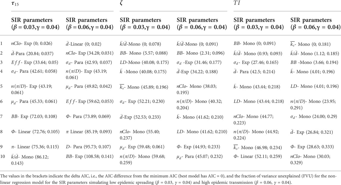
TABLE 1. The best ten NSIs to predict epidemic spreading for each spreading index.

FIGURE 1

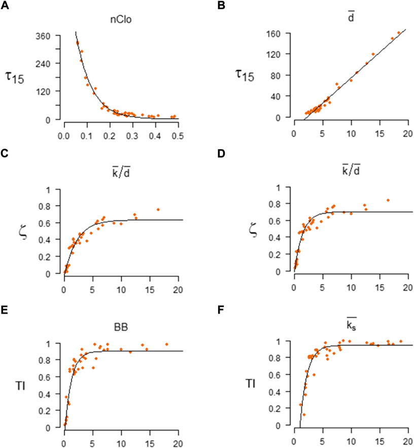
FIGURE 1. The best regression models of the Network Structural indexes (NSI) vs. Spreading Indicators (SI). Left column: the best regression models for SIR parameters β = 0.03 and γ = 0.04. Right column: the best regression models for SIR parameters β = 0.06 and γ = 0.04. Best for ${\tau }_{15}$: (A) ${\tau }_{15}$ as a function of the average normalized node closeness $nClo$; the relationship is described by an exponential model ${\tau }_{15}=a\cdot e^{-b\cdot nCLO}$ with a = 751.31 and b = −14.38 (FVU = 0.026); (B) ${\tau }_{15}$ as a function of the average node distance $\overline{d}$; the relationship is described by a linear model ${\tau }_{15}=a\cdot \overline{d}+b$ with a = 9.66, b = −21.86 (FVU = 0.02). Best for $\zeta$: (C) Non-linear regression of $\zeta$ vs. $\overline{k}/\overline{d}$ index; the relationship is described by a mono-molecular function model $\zeta =a\cdot \left(1-b\cdot e^{-c\cdot \left(\overline{k}/\overline{d}\right)}\right)$ with a = 0.63, b = 1.05 and c = 0.46 (FVU = 0.078); (D) Non-linear regression of $\zeta$ vs. $\overline{k}/\overline{d}$ index; the relationship is described by a mono-molecular function model $\zeta =a\cdot \left(1-b\cdot e^{-c\cdot \left(\overline{k}/\overline{d}\right)}\right)$ with a = 0.7, b = 1.02 and c = 0.7 (FVU = 0.091). Best for $TI$: (E) Non-linear regression of $TI$ vs. $BB$ index; the relationship is described by a mono-molecular function model $TI=a\cdot \left(1-b\cdot e^{-c\cdot BB}\right)$ with a = 0.91, 1.13 and c = 0.87 (FVU = 0.091); (F) Non-linear regression of $TI$ vs. $\overline{k_s}$ index; the relationship is described by a mono-molecular function model $TI=a\cdot \left(1-b\cdot e^{-c\cdot {\overline{k}}_s}\right)$ with a = 0.95, b = 2.22 and c = 0.81 (FVU = 0.181). Structural indicators key: $nClo$ average normalized node closeness; $\overline{d}$ average node distance,$\overline{k}/\overline{d}$ index; $BB$ index, $\overline{k_s}$ average node coreness. Spreading indicators key: ${\tau }_{15}$ time to reach the 15% of infected nodes, $TI$ total fraction of infected, $\zeta$ normalized infected peak.

The pace of the disease ${\tau }_{15}$

When considering the initial pace of disease (${\tau }_{15}$), the best models use as explanatory variables the average normalized node closeness $nClo$ (in an exponential form, Figure 1A), for low epidemic transmission (β = 0.03), and the average node distance $\overline{d}$ (linear relationship, Figure 1B) for high epidemic transmission (β = 0.06). The ‘distance’ $d_{\mathit{uv}}$ between two nodes u and v is the minimum length of a path joining them [14]. In other terms, the “distance” between two nodes u and v is the shortest path length, i.e., the minimum number of links to travel between them [14]. The average node distance $\overline{d}$, also called characteristic path length, measures the mean number of links to travel along the shortest path among node pairs in the network [14]. Figure 1B shows, for the higher epidemic transmission rate, the strong positive linear relationship between $\overline{d}$ and ${\tau }_{15}$, indicating that the higher the average node distance $\overline{d}$, the higher the time to infect the 15% of the network nodes.

The node closeness (or closeness centrality) is a measure of centrality in a network, calculated as the reciprocal of the sum of the distances (shortest paths length) between the node and all other nodes in the network [32]. Usually, the node closeness centrality may be normalized by dividing it by the term $N-1$, where $N$ is the network nodes number. It follows that the normalized node closeness of node i is the inverse average distance from node i to all other nodes (See Supplementary Material S1.1). Therefore, the new NSI “average normalized node closeness” $nClo$, we propose in this study, can be viewed as a measure of how many close network nodes are to each other, and it is an alternative indicator of evaluating the node distance in the network. For these reasons, even for a lower epidemic transmission rate, it emerges a strong negative relationship between the distance among network nodes ($nClo$) and the pace of the spreading (lower ${\tau }_{15}$) (Figure 1B). Noteworthy, both $\overline{d}$ and $nClo$ return very high goodness of fitting models, by explaining almost the entire variability in the ${\tau }_{15}$ observations (FVU∼2%, see Table 1). Taking these results together, our analyses show that the most important network structural factor to predict initial spreading speed is the notion of node distance.

The infected peak $\zeta$

When considering the maximum number of concurrently infected nodes ($\zeta$), the best models use the predictor $\overline{k}/\overline{d}$ in a mono-molecular form for both low and high epidemic transmission (Figures 1C,D). The accuracy of the $\overline{k}/\overline{d}$ regression model is high, by explaining more than the 90% variability in the $\zeta$ observations for both low and high epidemic transmission (FVU < 10%, see Table 1). The network infected peak $\zeta$ quickly raises with $\overline{k}/\overline{d}$, and reaches a plateau for higher $\overline{k}/\overline{d}$ values. The $\overline{k}/\overline{d}$ index (originally $A/D$ index), as the ratio of the average node degree $\overline{k}$ (i.e., the average number of links per node) and the average node distance $\overline{d}$, was introduced in mathematical graph theory to encompass the topological complexity of the network [15]. Thus, the peak of infected individuals in the network $\zeta$, that is the peak prevalence of the epidemic, is positively related to network connectivity (average node degree $\overline{k}$), and it decreases as a function of the node distance ($\overline{d}$).

The total infected $TI$

When considering the overall number of nodes that have been infected during an epidemic ($TI$), for low epidemic transmission (β = 0.03) the best predictor is the $BB$ index in a mono-molecular form (Figure 1E). The $BB$ index was introduced by Bonchev and Buck [15] to improve the $\overline{k}/\overline{d}$ measurement, and it follows the same rationale, accounting for the ratio between the node degree and a measure of the node distance (i.e., the farness) in the network. Let’s define the “farness” of the node i as ${\nu }_i={\displaystyle \sum }_{j=1}^{N-1}{d}_{ij}$ , where $d_{ij}$ is the distance between node i and node j, the $BB$ index is $BB={\displaystyle \sum }_{i=1}^N\frac{k_i}{{\nu }_i}$ where $k_i$ is the node degree of i and the ${\nu }_i$ is the “farness” of the node i. We find that $TI$ follows a saturating function of $BB$ index, showing how the total number of infected individuals may increase with network connectivity (node degree $k$) and decrease as a function of the node distance (here measured by the farness $\nu$).

For high epidemic transmission (β = 0.06) the best predictor is the average node coreness $\overline{k_s}$, in a mono-molecular form (Figure 1F). Node coreness (or coreness centrality) is a node centrality measure that shares the nodes in different sub-networks called k-core. The k-core of a network is a maximal sub-network in which each node has at least degree k [5]. In other terms, the coreness of a node is k if it belongs to the k-core but not to the (k + 1)-core. Kitsak et al. [5] showed that nodes of higher coreness are “influential spreaders” in the network, i.e., the nodes located in the network core determine a higher speed of network spreading. On the other hand, the epidemic starting in the network core may cover a large number of nodes, and the coreness centrality may be an efficient measure to individuate the nodes acting as efficient spreaders [5]. In this research, we introduce the $\overline{k_s}$ index as the average value of node coreness to evaluate the global network spreading. We can interpret networks with higher $\overline{k_s}$ as compact structures, where nodes of a higher degree are also located in the core of the network. We find that $TI$ is well fitted by a saturating function of $\overline{k_s}$, showing how the total number of infected individuals may increase in networks of higher average node coreness. Nonetheless, we outline that the performance of $\overline{k_s}$ is only slightly better than the $\overline{k}/\overline{d}$ prediction, and the regression models return almost equal goodness of fitting, with almost the same AIC and FVU (Table 1).

Discussion

Our results show that to predict network spreading to consider the distance among nodes is more important than focusing on their connectivity level. The most usual NSI evaluating the connectivity level of the network, i.e. the average node degree $\overline{k}$ [13], return a poor prediction of the network spreading for all the three spreading indicators used in this study (Table 2). In specific, $\overline{k}$ is strongly ineffective to explain the initial speed of the spreading ${\tau }_{15}$ (FVU∼0.5, Supplementary Tables S2, S4).

TABLE 2

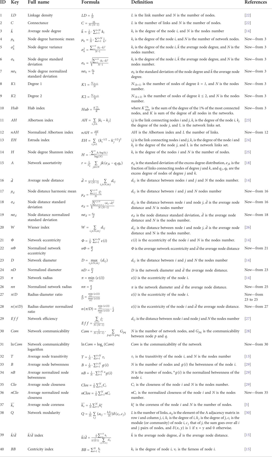
TABLE 2. Network structural indexes (NSI) list. For the NSIs from the literature is indicated the reference between square brackets; for the new NSIs is indicated “new” and the NSI number from they are derived.

This seems counter-intuitive, since higher connectivity levels correlate, on average, with lower node distance in the network [1–13].

Focusing $\overline{k}/\overline{d}$ and $BB$ indexes and ideal-types of the network structure we can figure out how the network connectivity level alone (i.e., the density of network links) may induce misleading predictions of the network epidemic spreading.

Both $\overline{k}/\overline{d}$ and $BB$ increase from the chain network (lower complexity), through the star network (medium complexity), to the complete network (maximum complexity) (Figure 2). Following this simplified ideal scheme, it is possible to figure out the classes of real-world networks and their epidemic spreading entity: it would be the lowest in chain-like network owing smallest average node degree $\overline{k}$ and highest average distance $\overline{d}$ (or farness $\nu$), average in the star network owing $\overline{k}$ similar to the chain network, but lower $\overline{d}$, and highest in the complete network, that maximize $\overline{k}$ and minimize $\overline{d}$ (or farness $\nu$).

FIGURE 2

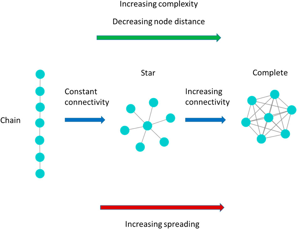
FIGURE 2. Model network examples of increasing complexity following Bonchev and Buck [16] theory of network complexity. When evaluating the complexity of the network with the rationale of the network structural indexes $A/D$ and $BB$ [16], the chain network is of lower complexity and low spreading pace, the star network is of intermediate complexity and medium spreading pace, and the complete network is the structure of maximum complexity, with the fastest spreading pace. The node distance always decreases with increasing complexity, i.e., passing from the chain to the star, and passing from the star to the complete network. Nonetheless, the node connectivity (links per node) holds constant passing from the chain to the star network, whereas increasing from the star to the complete network.

In particular, the higher spreading of the star network with respect to the chain network, hence these ideal-types of network show similar network connectivity, they present very different node distance, allows to explain how the network connectivity alone may not be a reliable predictor of the spreading entity, and networks of similar connectivity level may present very different spreading entity. On the other hand, our outcomes show that the magnitude of the de-correlation between connectivity and node distance of the real-world networks may be higher enough to make the network connectivity alone a scarce predictor of the epidemic spreading.

This outcome is particularly important in the context of the epidemic spreading, such as the SARS-Cov2 research. Important and recent research by Thurner and colleagues [11] focusing SIR epidemic spreading on networks showed that classic epidemiological models formulated as differential equations, and based on the mean-field approximation (assuming that every node/individual in principle can infect any other), can produce a misleading prediction of the real epidemic spreading extent. Consequently, Thurner et al. [11] questioned the applicability of standard compartmental models, which neglect the network structure, to describe the real epidemic spreading and the SARS-Cov2 containment phase.

From one side, the outcomes of our research strongly support the Thurner et al. [11] main statement showing how neglecting the network structure may perform erroneous predictions of the real epidemic spreading. On the other side, our results go further and extend the Thurner et al. [11] research outcomes. Here, we show that the network epidemic models investigating the SARS-Cov2 epidemic spreading focus on the network connectivity density as a main structural feature to parameterize network epidemic spreading, as done by Thurner et al. [11] and many recent network epidemic models [6, 8], may perform incomplete or even unrealistic spreading predictions.

Further, most of the non-pharmaceutical interventions (NPIs) implemented to curb the SARS-Cov2 epidemic follow the rationale to reduce social interactions [33, 34], that is to decrease the number of the network links. Our analyses suggest that implementing NPIs with the aim to space out the nodes, i.e., increasing the node distance in the network, would be a more effective strategy to halt the epidemic. This would translate into a reduced peak of infected individuals ($\zeta$) and, consequently, a lower number of infected individuals at the end of the epidemics ($TI$).

Last, we outline that many of the NSIs conceived in complex network science to encompass important network features that may potentially be leading to differently spreading entities, are not able to perform reliable predictions of the SIR epidemic spreading in real-world networks. The modularity ($Q$), the transitivity ($T$), the degree assortativity ($A$), and the different degree heterogeneity indicators (${\sigma }_k^2$, ${\sigma }_k$, $AH$, $EH$) of the network, that are assumed to influence network spreading [1, 2, 18, 20], return very low fitting model outcomes (Supplementary Tables S2, S4). For example, the degree assortativity $A$ returns FVU > 0.8 for all the spreading indicators, and the network modularity $Q$ shows FVU > 0.45 for all the spreading indicators. We argue that the weak outcomes of these NSIs may be due to two main reasons. On the one hand, in real-world networks, the aforementioned NSIs may present non-linear relationships among them, with contrasting effects in determining the network spreading entity. For example, Volz et al. [17] showed that the average node transitivity ($T$) alone is not always sufficient to determine the full epidemiological dynamics, since the epidemic spreading depends not only on the node transitivity, but also on the nature of the interactions with other network structural features [17].

On the other hand, our results show that the node distance is the most important factor affecting the network spreading. The aforementioned NSIs may not correlate with node distance, and, as explained above for the relationship between average node degree and node distance (Figure 2), real-world networks with the same value for these NSIs may present different node distance $\overline{d}$. For example, the relationship between degree assortativity ($A$) and node distance in the network is not linear, with contrasting effects on the epidemic spreading [18]. For this reason, real-world networks with similar values of these NSIs may present different spreading entities.

Materials and methods

Network structural indexes

In Table 2 we list the network structural indexes (NSIs) used in this study, a short definition, and their reference. For the NSIs coming from literature, we indicate the literature reference. For the new ones formulated in the present study by modifying or combining notions or indicators from literature, we list the indicators from which the new ones are derived. In the Supplementary Material S1.1, we furnish the extended definition of each network structural indicator.

Real-world complex networks database

We analyzed a set of 50 high-quality real-world networks from different fields of science (see Supplementary Material S1.2). The number of real-world networks for different areas of science is: road transportation 6, airports transportation 2, cargo-ship transportation 1, biological 4, ecological 2, social 13, citation 2, phone 2, internet 5, financial 1, computers 9, email 3. The complete list of real-world networks with network type and reference is in Supplementary Table S1.

The susceptible–infectious–recovered dynamic epidemics model

We used a susceptible-infected-recovered (SIR) model to numerically simulate the spreading entity over real-world networks. Type SIR models can successfully predict the dynamics of many infectious diseases. See Keeling and Rohani [35] for an overview. When considering SIR models over a network, at any time, a node can be in one of three possible compartments: susceptible (S), infected (I), and recovered (R). If a node/individual is infected, it will infect susceptible nodes linked to it with a transmission rate, β. An infected node/individual stays infectious on average for γ⁻¹ consecutive days, i.e., recovers with a rate equal to γ. Recovered node/individual can no longer infect others and its state will no longer change, which is equivalent to assume that immunization does not vanish in the considered time horizon. We initialized the system by fixing all nodes/individuals as susceptible except one, randomly chosen, whose state is set as infected. The system dynamics can then be solved and permit to model the epidemics evolution over time. To simulate the SIR spreading on a network we used the NDlib Python library presented in Rossetti et al. [36]. We fix the SIR parameters β equals 0.03 or 0.06, and γ = 4. We adopt two different transmission rate values of parameter β to describe low and high epidemic transmission. Higher values of β represent epidemics with higher transmissibility. We chose relatively small values for β, according to Kitsak et al. [5], so that the infected percentage of the population in the network remains small and the simulation can outline the role of the network structure for the spreading. In the case of larger β values, where spreading can reach a large fraction of the population in a few steps, the spreading would cover almost all the network in a few time steps thus hiding the role of topological structure to affect the pace of the spreading. For each real-world network, we implemented 10³ independent SIR simulations each with a different node/individual initially infected.

The pace of the epidemic spreading can also be evaluated by the time to infect a given part of the population [37]. We define the time to reach the 15% of infected nodes in the network. ${\tau }_{15}$ corresponds to the time steps of the SIR simulation necessary to have 15% of infected nodes (both considering the currently infected nodes and the recovered ones). The lower is the time to infect the fixed fraction of nodes/individuals, the faster is epidemic spreading.

Then, we assessed the pace of the epidemic spreading by the total number of individuals that have been infected ($TI$) at the end of the simulation, i.e., when there are no more infected nodes [5, 12] and by the maximum value of infected nodes in a given day ($\zeta$) [12]. The $TI$ indicator corresponds to the cumulative sum of new cases, which is equivalent to the number of recovered nodes at the end of the dynamics, when, by model construction, no more nodes can be infected. This is the indicator used to quantify the influence of a given node of the network in a SIR spreading process by Kitsak et al. [5] and to evaluate the efficacy of link removal strategies to curb the SIR spreading in social networks [12]. The $TI$ indicator provides an estimate of the spread of the disease within a population and it is likely to correlate with the number of severe, and possible fatal, cases. The $\zeta$ indicator, besides the evaluation of the spreading pace, it provides an estimate of the pressure over the sanitary system which might collapse, thus causing higher mortality probabilities of infected individuals, when a critical threshold is exceeded [12]. Since in epidemiology, “prevalence” is the fraction of a population currently infected [35], $\zeta$ can be defined as the maximum prevalence occurring during the epidemic simulations.

The list of the spreading indicators with their definition is in Table 3.

TABLE 3

TABLE 3. Spreading indicators used in this study.

The regression models

To estimate the goodness of the relationship between the spreading indicator value (response variable Y) and the network structural indicator value (independent variable or predictor X) we performed four types of regression models: linear, quadratic, exponential, and monomolecular.

Linear: $Y=aX+b$. It represents the simplest relationship between two variables i.e. one increases/decreases proportionally to the other.

Exponential: $Y=a\cdot e^{bX}$. It is used to model situations in which 1) the response of one variable, to the change of another, begins slowly and then accelerates rapidly without bound, or 2) its decay begins rapidly and then slows down to get closer and closer to zero. A multitude of situations can be modeled by exponential functions, such as investment growth, radioactive decay, atmospheric pressure changes, temperatures of a cooling object, etc.

Quadratic: $Y=a{X}^2+bX+c$. It represents those cases in which the maximum (or minimum) value of a variable is obtained at intermediate values of the independent variable. In biology, the growth rate of organisms is often modelled as a quadratic function of temperature. Such pattern can arise when the disease spread depends on the interaction of two processes which respond differently to the same NSI

Monomolecular (also known as Brody or Mitscherlich function): $Y=a\left(1-b\cdot e^{-cX}\right)$ where $b$ and $c$ are growth parameters, and $a$ is the asymptotic size [38]. The monomolecular is a special case of the generalised logistic function and it is a widely used growth curve model for saturating biological phenomena [38]. This typically occurs when other elements of the system interfere with the effect of the considered NSI and smooth its effect

The model selection criterion

We selected the best model using the Akaike information criterion (AIC) [31].

$AIC=2k-2\ln \left(\widehat{L}\right)(1)$

where k is the number of estimated parameters in the regression model (2 or 3 according to the regression model), and $\widehat{L}$ is the maximum value of the likelihood function for the model [31]. Given a set of candidate models for the data, the best model is the one with the minimum AIC value. Thus, AIC rewards goodness of fit (as assessed by the likelihood function), but it also includes a penalty that is an increasing function of the number of estimated parameters. The penalty discourages overfitting, which is desired because increasing the number of parameters in the model almost always improves the goodness of the fit. Minimization was performed using the R program function nlm (Gauss-Newton algorithm).

Eventually, to provide an easily interpretable measure of the goodness of the fitting model performances over network structural indexes (predictors), we computed the fraction of variance unexplained (FVU), calculated as:

$FVU=\frac{\sum _{i=1}^n\left(Y_i^o-Y_i^e\right)}{{\displaystyle \sum }_{i=1}^n\left(Y_i^o-\overline{Y^o}\right)}(2)$

where $Y_i^o$ is the observed value of the variable $Y_i$ (i.e. the observed spreading indicators value for the network i), $Y_i^e$ is the estimated value of the variable $Y_i$ (i.e., the value of the spreading indicators estimated by the fitting model for the network i), $\overline{Y^o}$ is the average observed value of the spreading indicators over the all networks set and $n$ is the total number of networks.

Data availability statement

Publicly available datasets were analyzed in this study. This data can be found here: The datasets analysed during the current study are available in the “Netzschleuder” repository [https://networks.skewed.de/], in the “Stanford Large Network Dataset Collection” repository [https://snap.stanford.edu/data/index.html], and in “The Colorado Index of Complex Networks (ICON)” repository [https://icon.colorado.edu/#!/].

Author contributions

BM, CD, AR, and BD conceived the research. BM, AR, and TM performed the analyses. All the authors wrote the manuscript.

Funding

This research is funded by a grant from the Italian Ministry of Foreign Affairs and International Cooperation. This project has received funding from the European Research Council (ERC) under the European Union’s Horizon 2020 research and innovation programme [grant agreement No. (816313)]. This work is supported by the Vietnam’s Ministry of Science and Technology (MOST) under the Vietnam-Italy scientific and technological cooperation program for the period 2021–2023. This work is supported by the Vietnam National University Ho Chi Minh City (VNU-HCM), Ho Chi Minh city, Vietnam under grant number B2018-42-01.

Acknowledgments

BM, TM, CD, and AR acknowledge the Italian Ministry of Foreign Affairs and International Cooperation. We are greatly thankful to Van Lang University, Vietnam for providing the budget for this study. We thank F. Sartori for helpful discussions.

Conflict of interest

The authors declare that the research was conducted in the absence of any commercial or financial relationships that could be construed as a potential conflict of interest.

Publisher’s note

All claims expressed in this article are solely those of the authors and do not necessarily represent those of their affiliated organizations, or those of the publisher, the editors and the reviewers. Any product that may be evaluated in this article, or claim that may be made by its manufacturer, is not guaranteed or endorsed by the publisher.

Supplementary material

The Supplementary Material for this article can be found online at: https://www.frontiersin.org/articles/10.3389/fphy.2022.1017015/full#supplementary-material

References

1. Pastor-Satorras R, Castellano C, Van Mieghem P, Vespignani A. Epidemic processes in complex networks. Rev Mod Phys (2015) 87:925–79. doi:10.1103/RevModPhys.87.925

CrossRef Full Text | Google Scholar

2. Pastor-Satorras R, Vespignani A. Immunization of complex networks. Phys Rev E (2002) 65:036104. doi:10.1103/PhysRevE.65.036104

PubMed Abstract | CrossRef Full Text | Google Scholar

3. Newman M. Spread of epidemic disease on networks. Phys Rev E (2002) 66:016128. doi:10.1103/PhysRevE.66.016128

PubMed Abstract | CrossRef Full Text | Google Scholar

4. Chen Y, Paul G, Havlin S, Liljeros F, Stanley H. Finding a better immunization strategy. Phys Rev Lett (2008) 101:058701. doi:10.1103/PhysRevLett.101.058701

PubMed Abstract | CrossRef Full Text | Google Scholar

5. Kitsak M, Gallos LK, Havlin S, Liljeros F, Muchnik L, Stanley HE, et al. Identification of influential spreaders in complex networks. Nat Phys (2010) 6:888–93. doi:10.1038/nphys1746

CrossRef Full Text | Google Scholar

6. Firth JA, Hellewell J, Klepac P, Kissler S, Jit M, Atkins KE, et al. Using a real-world network to model localized COVID-19 control strategies. Nat Med (2020) 26:1616–22. doi:10.1038/s41591-020-1036-8

PubMed Abstract | CrossRef Full Text | Google Scholar

7. Amaral MA, Oliveira MMd., Javarone MA. An epidemiological model with voluntary quarantine strategies governed by evolutionary game dynamics. Chaos Solitons Fractals (2021) 143:110616. doi:10.1016/j.chaos.2020.110616

PubMed Abstract | CrossRef Full Text | Google Scholar

8. Nishi A, Dewey G, Endo A, Neman S, Iwamoto SK, Ni MY, et al. Network interventions for managing the COVID-19 pandemic and sustaining economy. Proc Natl Acad Sci U S A (2020) 117:30285–94. doi:10.1073/pnas.2014297117

PubMed Abstract | CrossRef Full Text | Google Scholar

9. Hu Y, Ji S, Jin Y, Feng L, Eugene Stanley H, Havlin S. Local structure can identify and quantify influential global spreaders in large scale social networks. Proc Natl Acad Sci U S A (2018) 115:7468–72. doi:10.1073/pnas.1710547115

PubMed Abstract | CrossRef Full Text | Google Scholar

10. Pei S, Makse HA. Spreading dynamics in complex networks. J Stat Mech (2013) 2013:P12002. doi:10.1088/1742-5468/2013/12/P12002

CrossRef Full Text | Google Scholar

11. Thurner S, Klimek P, Hanel R. A network-based explanation of why most COVID-19 infection curves are linear. Proc Natl Acad Sci U S A (2020) 117:22684–9. doi:10.1073/pnas.2010398117

PubMed Abstract | CrossRef Full Text | Google Scholar

12. Bellingeri M, Turchetto M, Bevacqua D, Scotognella F, Alfieri R, Nguyen Q, et al. Modeling the consequences of social distancing over epidemics spreading in complex social networks: From link removal analysis to SARS-CoV-2 prevention. Front Phys (2021) 9:1–7. doi:10.3389/fphy.2021.681343

CrossRef Full Text | Google Scholar

13. Boccaletti S, Vito L, Moreno Y, Chavez M, Hwang D. Complex networks: Structure and dynamics. Phys Rep (2006) 424:175–308. doi:10.1016/j.physrep.2005.10.009

CrossRef Full Text | Google Scholar

14. Buckley F, Harary F. Distance in graphs. Redwood City, CA: Addison-Wesley Publishing Company (1990). doi:10.1201/b16132-64

CrossRef Full Text | Google Scholar

15. Bonchev D, Buck GA. Quantitative measures of network complexity. Complex Chem Biol Ecol (2005) 2005:191–235. doi:10.1007/0-387-25871-X_5

CrossRef Full Text | Google Scholar

16. De Domenico M, Granell C, Porter MA, Arenas A. The physics of spreading processes in multilayer networks. Nat Phys (2016) 12:901–6. doi:10.1038/nphys3865

CrossRef Full Text | Google Scholar

17. Volz EM, Miller JC, Galvani A, Meyers L. Effects of heterogeneous and clustered contact patterns on infectious disease dynamics. Plos Comput Biol (2011) 7:e1002042. doi:10.1371/journal.pcbi.1002042

PubMed Abstract | CrossRef Full Text | Google Scholar

18. Noldus R, Mieghem PV. Assortativity in complex networks. J Complex Netw (2015) 3:507–42. doi:10.1093/comnet/cnv005

CrossRef Full Text | Google Scholar

19. Miller JC. Spread of infectious disease through clustered populations. J R Soc Interf (2009) 6:1121–34. doi:10.1098/rsif.2008.0524

PubMed Abstract | CrossRef Full Text | Google Scholar

20. Salathe M, James J. Dynamics and control of diseases in networks with community structure. Plos Comput Biol (2010) 6:e1000736. doi:10.1371/journal.pcbi.1000736

PubMed Abstract | CrossRef Full Text | Google Scholar

21. Badham J, Stocker R. The impact of network clustering and assortativity on epidemic behaviour. Theor Popul Biol (2010) 77:71–5. doi:10.1016/j.tpb.2009.11.003

PubMed Abstract | CrossRef Full Text | Google Scholar

22. Bellingeri M, Vincenzi S. Robustness of empirical food webs with varying consumer’s sensitivities to loss of resources. J Theor Biol (2013) 333:18–26. doi:10.1016/j.jtbi.2013.04.033

PubMed Abstract | CrossRef Full Text | Google Scholar

23. Albertson MO. The irregularity of a graph. Ars Comb (1997) 46:219–25.

Google Scholar

24. Estrada E. Quantifying network heterogeneity. Phys Rev E (2010) 82:066102–8. doi:10.1103/PhysRevE.82.066102

PubMed Abstract | CrossRef Full Text | Google Scholar

25. Spellerberg IF, Fedor P. A tribute to Claude Shannon (1916–2001) and a plea for more rigorous use of species richness, species diversity and the ‘Shannon–Wiener’ Index. Glob Ecol Biogeogr (2003) 12:177–9. doi:10.1046/j.1466-822x.2003.00015.x

CrossRef Full Text | Google Scholar

26. Rouvray D. The rich legacy of half a century of the wiener index. Topology Chem (2002) 2002:16–37. doi:10.1533/9780857099617.16

CrossRef Full Text | Google Scholar

27. Latora V, Marchiori M. Efficient behavior of small-world networks. Phys Rev Lett (2001) 87:198701. doi:10.1103/PhysRevLett.87.198701

PubMed Abstract | CrossRef Full Text | Google Scholar

28. Estrada E, Hatano N. Communicability in complex networks. Phys Rev E (2008) 77:036111. doi:10.1103/physreve.77.036111

PubMed Abstract | CrossRef Full Text | Google Scholar

29. Freeman HE. A set of measures of centrality based on betweenness. Sociometry (1977) 40:35–41. doi:10.2307/3033543

CrossRef Full Text | Google Scholar

30. Clauset C, Newman MJ, Moore C. Finding community structure in very large networks. Phys Rev E (2004) 70:066111. doi:10.1103/physreve.70.066111

PubMed Abstract | CrossRef Full Text | Google Scholar

31. Burnham KP, Anderson DR. Multimodel inference: Understanding AIC and BIC in model selection. Sociol Methods Res (2004) 33:261–304. doi:10.1177/0049124104268644

CrossRef Full Text | Google Scholar

32. Marchiori M, Latora V. Harmony in the small-world. Physica A: Stat Mech its Appl (2000) 285:539–46. doi:10.1016/s0378-4371(00)00311-3

CrossRef Full Text | Google Scholar

33. Flaxman S, Mishra S, Gandy A, Unwin HJT, Mellan TA, Coupland H, et al. Estimating the effects of non-pharmaceutical interventions on COVID-19 in Europe. Nature (2020) 584:257–61. doi:10.1038/s41586-020-2405-7

PubMed Abstract | CrossRef Full Text | Google Scholar

34. Perra N. Non-pharmaceutical interventions during the COVID-19 pandemic: A review. Phys Rep (2021) 913:1–52. doi:10.1016/j.physrep.2021.02.001

PubMed Abstract | CrossRef Full Text | Google Scholar

35. Matt K, Pejman R. Modeling infectious diseases in humans and animals. New Jersey, United States: Princeton University Press (2008).

Google Scholar

36. Rossetti G, Milli L, Rinzivillo S, Sîrbu A, Pedreschi D, Giannotti F. NDlib: A python library to model and analyze diffusion processes over complex networks. Int J Data Sci Anal (2018) 5:61–79. doi:10.1007/s41060-017-0086-6

CrossRef Full Text | Google Scholar

37. Chen D, Lü L, Shang MS, Zhang YC, Zhou T. Identifying influential nodes in complex networks. Physica A: Stat Mech its Appl (2012) 391:1777–87. doi:10.1016/j.physa.2011.09.017

CrossRef Full Text | Google Scholar

38. Thornley JHM, France J. Mathematical models in agriculture: Quantitative methods for the plant, animal and ecological sciences. Wallingford, United Kingdom: Cabi (2007).

Google Scholar