Quantitative rheo-microscopy of soft matter

Direct observation of the microscopic material structure and dynamics during rheological shear tests is the goal of rheo-microscopy experiments. Microscopically, they shed light on the many mechanisms and processes that determine the mechanical properties at the macroscopic scale. Moreover, they permit for the determination of the actual deformation field, which is particularly relevant to assess shear banding or wall slip. While microscopic observation of the sample during mechanical probing is achieved by a variety of custom and commercial instruments, the possibility of performing quantitative rheology is not commonly available. Here, we describe a flexible rheo-microscopy setup that is built around a parallel-sliding-plate, stress-controlled shear cell, optimized to be mounted horizontally on a commercial microscope. Mechanically, soft materials with moduli ranging from few tens of Pa up to tens of kPa can be subjected to a variety of waveforms, ranging from standard step stress and oscillatory stress to more peculiar signals, such as triangular waves or any other signal of interest. Optically, the shear cell is designed to be compatible with different imaging methods (e.g. bright field or confocal microscopy). Most of the components of the shear cell are commercially available, and those that are not can be reproduced by a standard machine shop, easing the implementation of the rheo-microscopy setup in interested laboratories.

1 Introduction

Although somehow pleonastic to point out, one of the main characteristics of soft matter is precisely its softness. Every time we open the refrigerator and sink a teaspoon into yogurt, when we spread chocolate cream on a slice of bread, or when we squeeze out the tube an appropriate amount of toothpaste on the toothbrush we realize that all these materials are profoundly different from a classic liquid (e.g., water or apple juice) or solid (e.g., ceramic or metal). Moreover, many soft materials are also yield stress materials, effectively behaving as solids for small perturbations yet flowing like liquids in the presence of sufficiently large applied forces.

Such a rich rheological behavior arises from the underlying structural and dynamical complexity of the material constituents at one or more levels of organization. However, simultaneously characterizing the sample rheology, structure, and dynamics is not easily achieved experimentally. On one side, we have commercial rheometers, powerful and accurate instruments that grant access to the viscoelastic response of a material to a given strain/stress history in well-characterized geometries and in different shearing conditions; on the other side, we have commercial microscopes and scattering instruments that provide an accurate spatiotemporal map of the sample but are not conceived to be operated while the sample is mechanically perturbed.

This necessary trade-off has prompted several research groups to find a solution to combine the advantages of these approaches, ideally while maintaining a low level of instrumental complexity and a wide measurement range for rheological, structural, and dynamic parameters. Such combination has been implemented by relying on commercial rheometers [1–5], as well as on custom shear cells designed to work as rheometers [6–9]¹. The so-extracted information can be used for many purposes, such as correlating local material properties with the rheological response [14] or predicting materials failure from the analysis of failure precursors [15, 16].

In this work, building on seminal work by Aime et al. [8], we design, implement, and test a rheo-microscopy setup that is capable of performing a variety of rheological measurements while performing optical imaging of the sample via a commercial microscope. The core of the setup is a stress-controlled shear cell specifically designed for being used with different imaging configurations (e.g. bright field, confocal, …) and for maximizing the optical access of microscope objectives in the close vicinity of the sample. To make our setup as reproducible as possible, most of the optical, electronic, and mechanical cell components are commercially available, and the entire setup is controlled with National Instruments Labview. In particular, we opted for a commercial electronic signal generator to produce a variety of arbitrary stress patterns, which beyond the most standard oscillatory and step-like profiles also allow for more complex inputs, such as for instance triangular profiles. Our setup also allows triggering the optical detection with the mechanical input, thereby enabling us to perform for instance echo-imaging during oscillatory tests. While the tests presented here are meant to highlight the capabilities of our setup and give an idea of how it could be used, the setup could be pushed further. For instance, remaining in the framework of simple shear oscillation experiments, one could go beyond echo-imaging and study the intra-cycle dynamics to obtain information also on non-affine particle displacements; more complex shear profiles could also be used, such as chirped stress profiles or superpositions of simple signals.

Our rheo-microscopy setup is relatively simple to implement and quite robust to use for the multi-scale characterization of the link between the rearrangements occurring in soft materials under controlled stress and the evolution of their rheological properties.

2 Materials and methods

In a nutshell, the shear cell (Figure 1A) consists of a temporally controlled electrical current that feeds a magnetic actuator; the magnetic actuator exerts thus a controlled force on the upper part of the shear cell, which results in a rigid horizontal translation of the upper glass slide with respect to the lower one, which remains fixed. Similar to [8], the motion of the upper glass slide is accurately measured by optical cross-correlation of a speckle pattern that translates solidly with the upper glass slide (Figure 1B), so that one can impose a controlled stress profile and measure with nanometer precision the instantaneous strain. The optomechanical design is such that, when the cell is mounted on a commercial inverted microscope, all the sample planes comprised between the two glass slides can be visualized by proper positioning of the microscope objective (Figure 1C). In the following subsections, we describe in detail the different components and the typical data analysis procedures.

FIGURE 1

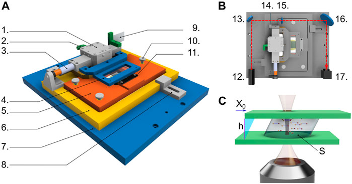
FIGURE 1. (A) Sketch of the key components of the shear cell: air bearing (1), inlet for compressed air (2), voice coil (3), holder for the upper glass slide (4), support of the lower glass slide (5), mounting base of the shear cell (6), microscope stage (7), clamping system fixing the cell mounting base to the microscope stage (8), ground glass (9), micrometric screws for controlling the gap distance h and the parallelism of the glass slides (10), pass-through hole enabling imaging with the underlying objective (11). The moving part of the shear cell, driven by the voice coil actuator, is composed by the moving parts of (1,3) plus parts (4,9). The entire block (5) lays on part (6) and its orientation can be finely tuned using the micrometric screws (10). (B) Top view of the shear cell also including the optical pathway and components used for the strain measurement via speckle field formation and detection: laser light source (12), mirror (13), ground glass solidly moving with the upper part of the shear cell (14), lens (15), mirror (16), and camera (17). (C) Sketch of the imaging geometry of the shear cell: the sample of cross-sectional area S is enclosed between the two glass slides placed at gap distance h; as the upper glass is moved by X₀ driven by the voice coil, the sample is sheared; the subsequent sample motion is monitored in time by imaging tracer particles with a long working distance objective, which can be positioned at different distance from the lower glass slide allowing to follow the sample dynamics at any selected plane z within the gap.

2.1 Shear cell description

The cell is built on the design described in Ref. [8]. It allows imposing a controlled stress, by means of a voice coil actuator, and accurately measuring the shear strain, by using optical speckle correlation analysis. While we keep these key elements unchanged, our implementation focuses on optimizing some aspects of the original design for use with a commercial inverted optical microscope, in our case the Nikon Eclipse Ti.

Beyond the obvious requirement of physically coupling the cell to the microscope while mounting it horizontally, which is fulfilled via a suitably designed microscope stage (7 in Figure 1A), another key requirement is maximizing the clear aperture on the bottom side to ensure the possibility of forming images within the samples at an arbitrary position within the entire sample thickness h. The mounting base (6 in Figure 1A) and the support of the bottom glass slide (5 in Figure 1A) are thus designed so to grant access to the tip of both long and short working distance microscope objectives, whose vertical position remains limited only by the presence of the bottom glass slide confining the sample. Another important design criterion concerns the shape of the glass slides confining the sample: on one side, one would want to use a large area of contact with the sample, which increases the effect of the applied force in the case of soft materials with small elastic modulus; on the other side, a large glass slide limits the free path of the moving stage, which in turn limits the maximum achievable strain. Our design, still making use of standard microscope slides for both the top and the bottom plates, allows us to flexibly change the shape of the bottom glass slide by suitable cutting. Here we use two options: a 60 mm × 24 mm slide mounted with the longer side orthogonal to the shear direction, which results in a maximum sample area of 4.5 cm² and a maximum moving stage free path of 25 mm; a second geometry, conceived to maximize the sample area in order to access to lower stresses, is obtained with the bottom slide measuring 65 mm × 26 mm, and mounted parallel to the top one (maximum sample area 12 cm², moving stage free path 1 mm). More information is provided in the Supplementary Information.

The top glass slide is mounted on a rigid frame (4 in Figure 1A), which translates rigidly and solidly with the body of the voice coil actuator (3 in Figure 1A). The rigid frame (4) has no other degrees of freedom and its distance from support (5) is varied by turning three micrometric screws that move the support (5); the three screws thus control the gap distance h and the parallelism between the two glass slides. The value of h is easily measured with the graduated vertical translator of the microscope, quantifying the distance between the two planes at which the upper side of the bottom glass and the lower face of the top glass can be sharply imaged. The parallelism between the two plates is checked by inspection of the fringe pattern arising when a red laser (638 nm diode laser, 0638L-13A, Integrated Optics) impinges on the empty cell. The doubly reflected light from the two glass slides generates an interference pattern whose fringes spacing is maximized when the two slides are parallel. In order to maximize the number of visible fringes, we use for the alignment a low magnification objective (Nikon Plan UW 2x/0.06, working distance 7.5 mm). With this procedure, the parallelism is granted with an accuracy of about 3 ⋅ 10^–4 rad (see Supplementary Information).

2.2 Stress application

Following [8], we feed an arbitrary current to a magnetic actuator (Moticont linear voice coil motor lvcm-013-032-02), which transforms the input current into a force by making use of a copper coil. This force is eventually exerted on the sample through the upper glass surface that is mounted on a stage sliding with reduced friction on an horizontal compressed-air rail (PI glide RB Linear Air Bearing Module A-101.050). As a distinctive element of our implementation, we use a commercially available source measure unit (SMU, NI PXIe-4138), mounted together with a NI PXIe-8840 controller in a NI PXIe-1071 chassis. The controller can operate under both MS Windows or proprietary National Instruments real time operating system. Real time operation is preferable to improve execution performances at high frequency; however, in this work we have been operating the device under MS Windows 10, due to the lack of support of our USB3 camera in the real time operating system. On the other hand, the adoption of a popular operating system like MS Windows 10 makes our setup easy to replicate, and very versatile.

We used NI Labview to program the SMU to supply currents up to 1 A with a noise-limited resolution of 1 μA, and with a microsecond time precision. Beyond standard continue (Section 4.4) and oscillatory (Sections 4.1 and 4.2) current (stress) profiles, a multitude of differently-shaped temporal stress profiles can be obtained, including triangular (Section 4.3) profiles, and modulated or chirped signals; the possibility to set more complex stress profiles could be also used for superposition rheology experiments [17]. Of note, we also found it useful to have the possibility to add an offset current to finely balance possible residual gravity effects due to the non-perfect leveling of the microscopy stage. Finally, since an SMU combines features of a power supply and digital multimeter device, we can impose a current profile I(t) and simultaneously read the voltage V(t) across the voice coil, which provides an estimate of the electric impedance of the magnet that we can use to monitor the magnet behavior checking for instance whether we approach its tolerance limit.

Calibration of the voice coil force-intensity ratio f_c was performed by using a precision balance measuring the force exerted by the coil for a fixed value of current in the range 10^–4 ≤ I ≤ 1 A (currents larger than 1 A were not used to avoid coil damage). In agreement with the results in Ref. [8] we found that f_c is essentially independent on the current intensity, but depends on the relative position d between the magnet and the coil. In our experiments, we choose to work around d = 12 mm (d = 0 mm corresponds to the magnet completely inside the coil), where for excursions up to 5 mm, we obtained f_c = (0.909 ± 0.002) NA⁻¹ (see Supplementary Information). In these conditions, for a typical gap of 300 μm, we obtain strains exceeding 800%. Also, considering typical sample areas of the order of 0.1 − 10 cm², the explored current range corresponds to an applied stress range of 0.1—10⁵ Pa, even though below 1 Pa (i.e. for currents smaller than 1 mA), we systematically observe a slight asymmetry between the amplitude of the stress obtained for negative and positive values of currents with the same amplitude (see Supplementary Information).

After calibration, the shear cell can impose controlled stress profiles to perform rheological tests (see Section 2.3 for the needed measurement of the strain) and for pre-conditioning of the sample before the tests. In the code we developed for the shear cell control and data acquisition, we implemented two rejuvenation pre-conditioning stress profiles: an oscillatory profile with constant frequency, and with large and constant stress maintained for an arbitrary time duration; and an oscillatory profile at constant frequency with stress decreasing from a large value to the value that the operator wants to use for the subsequent measurement. All the data in this work were obtained by using the high-stress oscillation rejuvenation protocol, imposing a rejuvenating strain of about 200%.

2.3 Speckle correlation based strain measurement

We implement a simple and compact optical correlation strain sensor (see Figure 1B) [8] to quantify the sample shear strain: a collimated laser beam (658 nm diode laser, DH658-60-3, Picotronic) impinges perpendicularly onto a ground glass (100 mm × 100 mm Square N-BK7 Ground Glass Diffusers, Thorlabs, homemade custom cut) that is rigidly mounted on the moving stage; a plano-convex lens with focal length 29.9 mm is positioned 33 mm after the ground glass and 330 mm before the speckle acquisition camera (Ximea MQ042MG-CM USB3.0 camera, sensor pixel size 5.5 µm, sensor size 2048 × 2048) in order to form a 10x magnified image of the ground glass, resulting in an effective pixel size of about half a micrometer. The image of the laser-illuminated ground glass appears covered in speckles whose size on the detector is $\approx 9$ µm (roughly corresponding to 2 pixels).

With this configuration, we acquire a sequence of images of a region of interest (ROI) of 2048 × 16 pixels, with the long side oriented along the direction of motion of the moving stage. From the spatial cross-correlation between consecutive frames the displacement of the speckle pattern, and thus of the moving stage, between the frames is recovered as the correlation peak position with a subpixel resolution of 0.02 pixels. With reference to the specific NI Labview implementation, a producer loop records the images and stores them in a buffer, and a consumer loop analyzes the correlations and determines the instantaneous velocity. For the aforementioned ROI, the consumer loop speed is the same as the producer one for acquisition frequencies up to 90 Hz. For larger acquisition frequencies, images accumulate in the buffer, and the speckle analysis must be performed offline. The dimension of the buffer allows us to easily keep a 1 KHz speckle pattern acquisition for a duration of some seconds and ensures that we can perform tests at tens of Hertz for hundreds of shear cycles. If needed, the limit for real-time analysis could be pushed at higher frequencies by using a camera supported by the real-time operating system described in Section 2.2.

2.4 Microscopy acquisition

All the experiments described in this manuscript are performed on fairly transparent samples. In this case tracer particles need to be added to monitor the local displacement field and to outline the occurrence of plastic rearrangements.

Imaging of the tracers is performed with a commercial optical microscope (Nikon Eclipse Ti), set for Koehler illumination. To minimize the contribution of particles that are not in the microscope object plane, the depth-of-focus is made as small as L_f ≃ 20 μm by keeping the condenser (NA = 0.52) diaphragm completely open. Images are acquired by a second Ximea MQ042MG-CM USB3.0 camera at the imposed acquisition frequency and stored in a circular buffer: while simultaneously performing rheology experiments, full frame (2048 × 2048 pixels) image acquisition at 10 Hz (25 Hz with 2 × 2 binning) can be performed without filling the RAM for at least 1 hour; full frame acquisitions at larger frequencies are possible but only for a few seconds. Imaging data presented in the present paper are acquired with a 20×, 0.45 NA long-working-distance objective, resulting in a field-of-view size of 563 × 563 µm².

2.5 Triggered image acquisitions

For rheology experiments with a periodic stress profile (e.g. for stress oscillation experiments), we implemented the possibility of microscopy images acquisitions in echo mode [11]: we acquire for each period a fixed integer number n of images and repeat a similar acquisition over a very large number of periods (typically 100 − 1000); the resulting video is then divided into its n stroboscopic components, each of them capturing the sample temporal evolution for ideally the same applied stress after exactly one period and multiples of it (echoes). As already pointed out in Ref. [11], the presence of tiny (less than 1 ms) mismatches between the stress and the sampling frequency may be negligible at the single period time scale but becomes important if the delay accumulates over a long measurement (order of 300 iterations), as it implies apparent drifts in the echo analysis.

To minimize such temporal mismatches, we use hardware triggering of the voice coil, the speckle camera, and the sample imaging camera. To this aim, we use the National Instrument SMU to send an output trigger at the end of every current signal period iteration. An operational amplifier in a non-inverting configuration increases the amplitude and duration (with a low-pass filter) of the trigger signal in order to make it detectable by the two cameras. Once the trigger signal is received, every camera acquires a fixed number of frames per period (typically 10 for the imaging camera and 50-80 for the speckle camera). The camera then awaits the following trigger signal before starting the subsequent acquisition sequence. In this way, any mismatch between the imposed and the effective acquisition frequencies does not accumulate a time delay between applied stress and acquired images, thus avoiding apparent drift in image acquisition. Moreover, the synchronization of the applied stress with the image acquisition reduces the uncertainty of the phase delay between the applied stress and the consequent measured strain. Without synchronization, the strain detection begins with the first acquired frame after the application of the stress, which would not give control of the starting phase. With triggering, the delay is given by the trigger precision δ_t ≃ 1 µs, which corresponds to an error on the phase delay that is bounded from above by δ_ϕ = 2πf_σδ_t, where f_σ is the imposed stress frequency. In typical experiments with f_σ < 100 Hz, one has δ_ϕ < 10^–3 rad (to be compared with δ_ϕ ≃ 10^–1 rad without trigger), an error that can be safely neglected, being smaller than the precision limit imposed by the finite number of acquired points per period.

2.6 Preparation and loading of the samples

To fill the shear cell with the sample, the upper glass slide support is easily unmounted, and both glass slides are carefully cleaned before sample loading. With the exception of the Sylgard sample (see below), all samples are prepared ex situ and subsequently placed in the shear cell by using a spatula or a pipette. The upper slide support is then put back in its place by carefully checking that the sample drop remains within the perimeter of the upper and lower glass. To assess the imposed stress σ = F/S from the applied force F, we measure the sample cross-sectional area S by imaging the sample once loaded using a smartphone. For this purpose, we position the smartphone on a holder placed at a distance that minimizes field distortions and parallax errors. Spatial calibration of the effective image pixel size is obtained by using as a reference length the known distance between the cell edges while the contour of the drop is obtained trough a manual polygonal segmentation using the Matlab drawnpolygon function. For samples subjected to evaporation, such as Carbopol, several pictures of the sample area are taken during the measurement in order to retrieve the area as a function of time. Tests with Carbopol samples over four consecutive hours revealed that tracking the temporal changes of S is of fundamental importance to obtain a correct rheological characterization of the sample, as changes in S dominate over the moduli changes due to the water evaporation-induced concentration change of the sample, which turned out to be negligible. Contact angles different from π/2 between the sample and the glass slides can introduce errors in the evaluation of the effective area S due to the presence of a meniscus (especially for liquid samples like glycerol and silicon oil). A more precise evaluation of the area can be in principle obtained for non-evaporating samples by adding an accurately known volume of sample in the shear cell, but sample viscosity makes this operation practically quite difficult in most cases. Another possibility, beyond the aim of the present paper, is an in-depth study on possible treatments of the glass slides to reach for a given sample a contact angle of π/2 in order to reduce the meniscus and thus the error in the evaluation of S. Tracers have been dispersed only in the Carbopol samples since Sylgard and the purely viscous liquids have been only used to verify the capability of the shear cell in properly measuring the macroscopic rheology of well-characterized samples.

2.6.1 Viscous liquids

In order to test the behaviour of the cell with simple viscous fluids, we used glycerol (Sigma Glycerol for molecular biology, $\ge 99.0\%$) and silicon oil (BlueStar Silicon Bluesil 47V30000, nominal viscosity 30 Pa⋅s). Frequency sweeps at T = 23.5 ± 0.5°C (the same at which the shear cell measurement reported in Section 4.1 were performed) performed with an Anton Paar Physica MCR300 rheometer in a cone and plate geometry provided a viscosity η = 29.2 ± 0.3 Pa⋅s for the silicon oil. Glycerol at 99% is expected to have a nominal viscosity of 1.19 Pa⋅s at room temperature (20 °C) [18]. However, the high hygroscopicity of glycerol at concentrations close to 100% causes the real viscosity of the sample during the measurement to be noticeably lower [19].

2.6.2 Sylgard

Sylgard samples are prepared by adding the curing agent (Sylgard 184 curing agent, Dow Corning) to the base (Sylgard 184 Base, Dow Corning) in the proportion 1:50. The components are mixed directly on the bottom slide of the shear cell, by keeping the drop shape as circular as possible. The upper slide is then closed and the sample is left to dry at room temperature for at least 48 h. Because of the strong adhesion of the Sylgard on glass, we used untreated microscope slides as cell glass slides.

2.6.3 Carbopol

For preparing the Carbopol samples we followed the procedure described in [11]: samples are prepared at the desired concentration by dispersing Carbopol 971P NF (Lubrizol) powder in MilliQ water while stirring for several days and controlling the pH through the addition of NaOH 10 M. After preparation, tracers (Polystyrene particles of 2 µm diameter, Microparticles GmbH) are dispersed at a volume fraction of 0.05%. The size of the tracers was chosen to be slightly larger than the mesh size of the sample, as discussed in Ref. [11]. Dispersion is reached by mixing with a spatula and by spinning for a few seconds on a centrifuge to get rid of gas bubbles. In order to reduce sample-glass slip, both the glass slides are frosted with sandpaper, by carefully leaving unfrosted a small circular area of diameter 5 mm to allow optical imaging.

3 Data analysis

3.1 Extracting the macroscopic rheological properties of the sample

Measuring the speckle displacement on the camera provides a measure of the displacement $X_0\left(t\right)$ of the ground glass and consequently the displacement of the upper glass slide of the cell (see Figure 1A). The speckle displacement (in pixel) between two consecutive frames is calculated with a cross-correlation analysis that gives a resolution of 0.02 pixels (see also Section 2.3). Displacements between non-consecutive images are obtained as sums of displacements between consecutive ones. The effective pixel size is measured by displacing the moving stage along its whole range while acquiring the speckle field. The corresponding displacement (in pixels) obtained from the speckle correlation analysis is then compared with the effective distance travelled by the moving stage measured with a caliper. From this procedure, we obtain an effective pixel size d_pixel = 0.49 ± 0.01 µm. Considering the aforementioned subpixel resolution and speckle ROI dimensions (Section 2.3), our device is therefore able to detect displacements ranging from 10 nm to 500 µm. For a typical gap of 300 µm and a typical speckle image acquisition frequency of 80 Hz, one has a minimum measurable strain of 3 ⋅ 10^–5 and a maximum measurable strain rate of 133 s⁻¹. In practice, the minimum detectable strain is larger due to mechanical noise sources, such as vibrations and air flows in the vicinity of the cell.

From $F\left(t\right)$ and $X_0\left(t\right)$, the stress and strain time evolution are directly accessible as $\gamma \left(t\right)=X_0\left(t\right)/h$ and $\sigma \left(t\right)=F\left(t\right)/S$, respectively. In the linear range, we expect that the response to an applied oscillatory stress $\sigma \left(t\right)=F\left(t\right)/S={\sigma }_0\sin \omega t$ with frequency ω and amplitude σ₀ = F₀/S is an oscillatory strain $\gamma \left(t\right)=X_0\left(t\right)/h=A_0\sin \left(\omega t-\varphi \right)$ with the same frequency and a phase delay ϕ. In this case, the sample complex modulus G^∗ is obtained as the ratio between stress and strain

$G^{\ast }=\frac{\sigma }{\gamma }=\frac{{\sigma }_0}{{\gamma }_0}{e}^{i\varphi }.(1)$

Elastic and loss moduli can be recovered as the real and imaginary part of G^∗ respectively

$\left\{\begin{array}{c}{G}^{\prime }=\frac{{\sigma }_0}{{\gamma }_0}\cos \varphi \hfill \\ G^{″}=\frac{{\sigma }_0}{{\gamma }_0}\sin \varphi \hfill \end{array}\right.(2)$

In principle, once ϕ, γ₀ = A₀/h and σ₀ are known, the elastic and loss moduli can be directly recovered. In practice, we find that air movements around the sliding stage can introduce random drifts, whose effects are negligible for stiff samples but can become important when G = |G*| ≤ 100 Pa. Such drifts can be corrected for through a suitable fit with the expression

$X_0\left(t\right)=A\sin \left(\omega t-\phi \right)+f_{\mathit{pol}}\left(t\right)(3)$

where $f_{\mathit{pol}}\left(t\right)$ is a polynomial function accounting for the drift contribution (see Supplementary Information). By fitting the function in Eq. 3 to the measured displacement X₀(t), we obtain an estimate of the drift term $f_{\mathit{pol}}\left(t\right)$. A simple sinusoidal function $A_0\sin \left({\omega }_{0}t-\varphi \right)$ is then fitted to the corrected data $X_0^{\prime }\left(t\right)=X_0\left(t\right)-f_{\mathit{pol}}\left(t\right)$. The best fitting parameters A₀, ω₀, and ϕ, correspond to the displacement amplitude, the oscillation frequency, and the relative phase between the oscillatory forcing signal and the response displacement, respectively. For ease of notation, we will indicate in the following the upper glass displacement corrected by drift with X₀.

Typical results of the applied force $F\left(\omega t\right)$ and the resulting displacement obtained for our perfectly viscous and elastic reference systems, silicon oil and Sylgard, are shown in Figure 2. As expected, the viscous sample displays a phase shift of π/2 while the elastic one is in phase with the forcing signal.

FIGURE 2

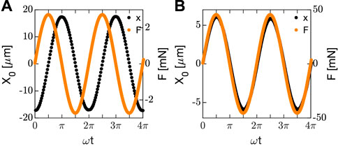
FIGURE 2. Applied force (orange) and resulting displacement (black) obtained measuring silicon oil at ω = 2.46 rad/s (A) and Sylgard at ω = 0.1 rad/s (B).

3.1.1 Inertia and friction

In a stress-controlled rheology experiment, a prescribed temporal profile of shear stress values is applied to the sample and the resulting deformation is measured as a relative strain. The motion of the moving stage of our shear cell is, however, not only determined by the applied stress and the material mechanical properties, but also by inertial and dissipative contributions of the shear cell components. These contributions are particularly relevant in oscillatory measurements and can be quantified with calibration measurements performed with the empty cell. For these, we can write

$m\ddot{X_0}=F-\xi \dot{X_0}+F_{fr}(4)$

where m is the mass of the moving stage, responsible for the inertial contribution to the dynamics, ξ is the viscous drag inherent to the shear cell, and F_fr is a sliding friction contribution. The latter is ideally equal to zero in a perfect frictionless device. In real devices, however, it is a constant force always opposing the direction of motion, which needs to be accounted for.

Using a magnet to apply an oscillating force F = F₀e^iωt at frequency ω, we expect in first approximation a sinusoidal displacement with the same frequency, as $X_0=A_0{e}^{i\left(\omega t-\varphi \right)}$. The sliding friction contribution is therefore expected to be a square wave $F_{fr}=-F_{fr,0}\mathrm{sign}\left(\dot{X_0}\right)$, where F_fr,0 is the modulus of the sliding friction. For the sake of analytical simplicity, we expand F_fr in Fourier series arresting to the first order, thus approximating the sliding friction contribution to a sinusoidal oscillation $F_{fr}=-i{F}_{fr,0}{e}^{i\left(\omega t-\varphi \right)}$ in phase opposition to the velocity $\dot{X_0}=i\omega A_0{e}^{i\left(\omega t-\varphi \right)}$. By making explicit the time dependencies and dividing by $e^{i\left(\omega t-\varphi \right)}$, Eq. 4 becomes:

$F_0{e}^{i\varphi }=-m{\omega }^2{A}_0+i\left(\xi \omega A_0+F_{fr,0}\right)(5)$

that can be rewritten as:

$\left\{\begin{array}{c}{F}_0\cos \varphi =-m{\omega }^2{A}_0\hfill \\ F_0\sin \varphi =\xi \omega A_0+F_{fr,0}\hfill \end{array}\right.(6)$

We show in Figure 3A the results obtained from a frequency sweep performed with the empty cell for $\mathrm{R}\mathrm{e}[F/X_0]=\left(F_0/A_0\right)\cos \varphi$ (circles) and $\mathrm{I}\mathrm{m}[F/X_0]=\left(F_0/A_0\right)\sin \varphi$ (triangles). Within the investigated frequency range, the phase-shifted component $\left(F_0/A_0\right)\sin \varphi$ is always smaller in absolute value than the in-phase component $\left(F_0/A_0\right)\cos \varphi$; this shows that the inertial contribution always dominates over the viscous one. As expected, the in-phase response is compatible with a quadratic dependence on ω; the corresponding best-fitting curve is shown as a red continuous line. From the fit, a value of m = 0.314 ± 0.006 Kg is obtained.

FIGURE 3

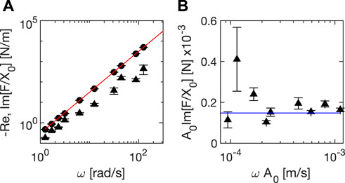
FIGURE 3. (A) − Re [F/X₀] (circles) and Im [F/X₀] (triangles) as a function of ω from a frequency sweep experiment performed with the empty cell. Continuous red line is a quadratic fit of − Re [F/X₀], which provides the estimate m = 0.314 ± 0.006 Kg for the mass of the moving stage. (B) A₀Im [F/X₀], recovered from the same data of (A), as a function of the maximum velocity ωA₀.

By contrast, the phase-shifted contribution is not increasing linearly with frequency, as one would expect for viscous friction only; this suggests that sliding friction has to be taken into account. In order to assess the relative importance of the two different dissipative contributions, we report F₀ sin ϕ as a function of ωA₀ in Figure 3B. Clearly, F₀ sin ϕ is almost frequency independent, which is expected for sliding friction contributions. Thus, viscous dissipation appears to be negligible compared to dissipation by sliding friction. We can therefore determine the value of the sliding friction contribution as $F_{fr,0}={⟨F_0\sin \varphi ⟩}_{\omega A_0}=0.15\pm 0.03$ mN.

By taking these results into account, we can rewrite Eq. 2 to include inertia and dissipation effects, which gives:

$\left\{\begin{array}{c}{G}^{\prime }=\frac{{\sigma }_0}{{\gamma }_0}\cos \varphi +I{\omega }^2\hfill \\ G^{″}=\frac{{\sigma }_0}{{\gamma }_0}\sin \varphi -\frac{F_{fr,0}}{{\gamma }_{0}S}\hfill \end{array}\right.(7)$

where $I=m\frac{h}{S}$. In this work, we use these equations to extract the viscoelastic moduli from stress oscillation experiments, which requires that inertia and sliding friction are systematically characterized with the empty cell before performing a measurement.

The procedure just described operates a correction of G″ for the sliding friction contribution, which is approximated with a sinusoidal instead of a square wave. We opted for such a simplified treatment because it enables us to operate a correction directly on the fit parameters using Eq. 7 instead of Eq. 2. An alternative route would consist in directly subtracting the square wave friction contribution from X₀ before the fit. This procedure would introduce an additional fitting step of the strain to recover ϕ and properly subtract the friction contribution, before fitting again the strain data. Our simplified correction turns out to be more effective, as it lowers by half a decade (from 5 ⋅ 10^–3 N to 10^–3 N) the minimum applied force that can be considered to result in reliable measurements (see next section). We thus decided not to launch a more rigorous treatment, which would result in additional distortions of the strain profile for applied forces lower than 10^–3 N, where static friction contributions would also be needed to be taken into account.

3.2 Analysis of the microscopy images: mapping the effect of shear at the local scale

The local counterpart of the macroscopic response of the material is investigated through the analysis of the tracer dynamics imaged with the camera. By shifting the object plane we can map the microscopic dynamics across the entire gap (z-scan), and extract information about the affine and non-affine components of the particle displacement. This information can be used to obtain a characterization of the mesoscopic shear profile across the gap (i.e. in the gradient direction) as well as of the microscopic particle rearrangements in the shear and vorticity directions. Microscopy images can be analyzed with a variety of approaches [20], including particle tracking (PT) [21, 22], particle imaging velocimetry (PIV) [23, 24], and differential dynamic microscopy (DDM) [25, 26] methods.

3.2.1 Mapping the effective strain across the sample gap

A key feature of our rheo-microscopy approach is that we can measure the effective strain across the gap by tracking the tracers at different positions in z. This feature is particularly useful to inspect for slip and shear banding [27]. To have a certain slip of the sample at the cell boundaries is often the case, and generally leads to an overestimation of the strain measured macroscopically with both shear cells and rheometers. Similarly, the non-linear behavior of many soft materials involves shear banding, which also introduces important deviations from the ideal strain profile.

To recover the effective strain within the sample during oscillatory experiments, we first measure the apparent gap $\tilde{h}$ as the difference between the two positions along the microscope optical axis for which we obtain two sharp images of the top and bottom glass slides with the sample loaded on the cell. As the refractive index of the sample is always larger than 1, such measurement returns an apparent gap lower than the real gap h measured with the empty cell, an effect known as focal shift. Once the apparent gap is determined, we perform a z-scan with a given step length, typically of 25 μm, moving downwards from the upper glass. In a typical experiment, we impose an oscillatory stress at a given amplitude σ₀ and frequency ω on the top plate; the stress is thereby transmitted to all planes (even in case of wall slip or shear banding). For each position ${\tilde{z}}_i\in [0,\tilde{h}]$ of the apparent gap we then recover the effective strain by applying the procedure introduced for a strain-controlled cell in [11]. In short, we acquire a fast time-lapse of a duration at least of three oscillation periods (see Supplementary Video SM1), and we evaluate the displacement profile $\mathbf{X}({\tilde{z}}_i,t)$ by cross-correlating consecutive images of the acquired stack. By fitting $\mathbf{X}({\tilde{z}}_i,t)$ to a sinusoidal function of time, we estimate the displacement amplitude $A({\tilde{z}}_i)$, which we map onto the real gap by using the simple relation $z_i=\widetilde{z_i}h/\tilde{h}$. We then evaluate the local effective z-dependent strain as

$\gamma \left(z\right)=\partial A\left(z\right)/\partial z.(8)$

Representative displa-cement profiles A(z) obtained in oscillation experiments (ω = 2π rad/s) with Carbopol 0.5% and 5% are shown in respectively Figures 4A,B, where A(z) is normalized by the strain amplitude A₀ estimated from the speckle correlation analysis. Different datasets refer to different values of the applied stresses: σ ∈ [1.5 − 17] Pa for the 0.5% sample, and σ ∈ [11 − 190] Pa for the 5% sample. For both samples, the deformation profiles indicate the absence of shear banding even at the yielding transition, which occurs at σ ∼ 15 Pa (0.5%) and σ ∼ 130 Pa (5%). Compared to the data obtained for Carbopol 5%, A(z)/A₀ obtained for Carbopol 0.5% clearly deviates from the expected strain profile (green dashed line in Figures 4A,B), denoting a notable, weakly stress-dependent slip. Close to the cell boundaries (gray regions in Figure 4), our results are affected by the depth-of-focus L_f of the microscope (see Section 2.4), which defines the thickness of the axial region contributing to a microscope image centered around the ideal object plane. When such plane lies in the region defined by z ∈ [L_f/2, h − L_f/2], the contributions to the amplitude displacements from the planes above and below the ideal object plane substantially average out for symmetry. However, such cancellation does not occur close to the top and bottom slides (gray regions in Figure 4), and cross-correlation analysis in the top (bottom) region leads systematically to a lower (higher) estimation of the actual amplitude. Within this frame, both the axial resolution and the size of the excluded volume can be improved using a higher numerical aperture objective, providing a smaller L_f. Even though a further way to enhance the z resolution would be to use confocal microscopy, we did not find this issue to be a limiting factor in our experiments, as we restricted our attention only to the region z ∈ [L_f/2, h − L_f/2] (white regions in Figure 4). This approach remains compatible with our cell and can be taken in case one is interested in systems presenting heterogeneity of the deformation field on the scales of a few microns [12, 28].

FIGURE 4

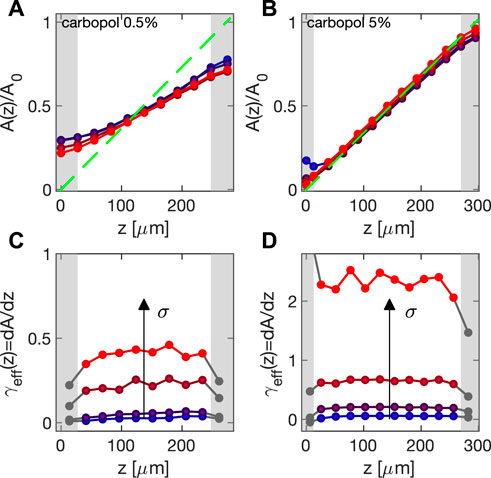
FIGURE 4. (A,B) Deformation profile A(z) normalized by the macroscopic deformation amplitude A₀ as determined from the speckle correlation analysis. Data obtained for Carbopol 0.5% (A) and 5% (B) at ω = 2π rad/s for stress amplitudes ranging from σ = 1.5 Pa (blue) to σ = 13 Pa (red) for Carbopol 0.5%, and from σ = 11 Pa (blue) to σ = 190 Pa (red) for Carbopol 5%. Green dashed line denotes the ideal strain profile presumed in any macroscopic rheology experiment. Gray patches mark gap regions in which the amplitude estimation is biased by finite depth-of-focus. (C,D) Corresponding effective local strain γ_eff(z), evaluated using relation 8 for Carbopol 0.5% (C) and 5% (D). Gray marks correspond to the z for which the estimation of the local strain is not reliable.

3.2.2 Echo-dynamics in oscillation experiments

To study irreversible plastic rearrangements within the sample, we use the echo scheme described in Section 2.5). In this configuration, an oscillatory stress with amplitude σ₀ and frequency ω is imposed and a long image sequence of a fixed integer number n of images for each period is acquired. For each acquisition we therefore obtain n different echo sequences that correspond to different phases of the oscillatory stress. To estimate the shear-induced echo-dynamics, we consider each value of the phase separately. For each of them, we first calculate a background image I₀(x) as the median image over the entire image sequence, which we subtract from all the images. The so-obtained sequence is then rigidly registered by using the Image-J plugin Stack-Reg, and choosing as a reference image the one that lies in the middle of the acquisition. At the end of the registration, we save the transformation matrix of each image in the sequence, which we subsequently use for pre-processing the images in MATLAB, where the rest of the analysis is performed by exploiting echo-particle tracking and echo-differential dynamic microscopy (Echo-DDM) as briefly presented below and described in more detail in [11].

3.2.2.1 Echo-particle tracking

The registered images are convoluted with a Wiener filter (standard deviation 2 μm) and subsequently analyzed with a particle-tracking code developed in Ref. [22] and available online² to obtain single particle trajectories [x⁽ⁱ⁾(t), y⁽ⁱ⁾(t)] (typically ∼ 500). During shearing, we find that the displacement is not always perfectly uniform within the field-of-view: on top of a constant average translation a more complex displacement field is also observed. These non-rigid contributions result from local meso- and macroscopic rearrangements probably due to local differences in the adhesion of the sample on the glass slides and effects of finite size and inhomogeneities of the sample. These non-rigid contributions, (which would be undetectable in a standard rheological measurements) although much smaller than the rigid translation due to shearing, become relevant in echo mode, as they lead to a ballistic-like contribution to the particle dynamics. In order to reduce their effect, we adopted a mutual-particle tracking approach [29].

Considering two particles i = 1, 2 subjected to local drifts u (1) and u (2), respectively, we can write the particle positions at time t along the vorticity (x) and shear (y) direction as:

$x^{\left(i\right)}\left(t\right)=x_0^{\left(i\right)}\left(t\right)+u_x^{\left(i\right)}\left(t\right),$

$y^{\left(i\right)}\left(t\right)=y_0^{\left(i\right)}\left(t\right)+u_y^{\left(i\right)}\left(t\right),$

where $(x_0^{(i)},y_0^{(i)})$ is the true particle dynamics. If the particles are close enough so that are subjected to the same velocity field u⁽ⁱ⁾ and hydrodynamic correlations are negligible, the mean square displacement (MSD) evaluated over the relative position of the particles [Δx^(i,j), Δy^(i,j)] = [x⁽ⁱ⁾(t) − x^(j)(t), y⁽ⁱ⁾(t) − y^(j)(t)], along the vorticity and shear directions yields to:

$MS{D}_v\left(\mathrm{\Delta }t\right)=\frac{1}{2}\langle |\mathrm{\Delta }{x}^{\left(i,j\right)}\left(t+\mathrm{\Delta }t\right)-\mathrm{\Delta }{x}^{\left(i,j\right)}\left(t\right){|}^2\rangle =\langle |x_0^{\left(i\right)}\left(t+\mathrm{\Delta }t\right)-x_0^{\left(i\right)}\left(t\right){|}^2\rangle (9)$

$MS{D}_s\left(\mathrm{\Delta }t\right)=\frac{1}{2}\langle |\mathrm{\Delta }{y}^{\left(i,j\right)}\left(t+\mathrm{\Delta }t\right)-\mathrm{\Delta }{y}^{\left(i,j\right)}\left(t\right){|}^2\rangle =\langle |y_0^{\left(i\right)}\left(t+\mathrm{\Delta }t\right)-y_0^{\left(i\right)}\left(t\right){|}^2\rangle$

where the average is performed over all initial times t, all the pair of particles (i, j) within a distance d (typically $\sim 20\mu m$) such that $⟨u_{x,y}^{(i)}(t+\mathrm{\Delta }t)u_{x,y}^{(j)}(t)⟩=u_{x,y}^2\delta (\mathrm{\Delta }t)$ or equivalently $u_{x,y}^{(i)}\simeq u_{x,y}^{(j)}$, and over all the echo phases.

Similarly, we can compute the particle mutual-displacement probability distribution functions (PDF), along the vorticity and shear direction, respectively:

$P_v\left(\mathrm{\Delta }x,\mathrm{\Delta }t\right)=⟨\delta \left[\mathrm{\Delta }x-\left(\mathrm{\Delta }{x}^{\left(i,j\right)}\left(t+\mathrm{\Delta }t\right)-\mathrm{\Delta }{x}^{\left(i,j\right)}\left(t\right)\right)\right]⟩,(10)$

$P_s\left(\mathrm{\Delta }y,\mathrm{\Delta }t\right)=⟨\delta \left[\mathrm{\Delta }y-\left(\mathrm{\Delta }{y}^{\left(i,j\right)}\left(t+\mathrm{\Delta }t\right)-\mathrm{\Delta }{y}^{\left(i,j\right)}\left(t\right)\right)\right]⟩.(11)$

3.2.2.2 Echo-DDM

As introduced and described in [11], echo-DDM consists of a differential dynamic microscopy (DDM) analysis of each registered echo image sequence [25, 26]. In brief, we compute the 2D spatial Fourier transform $\widehat{I}(\mathbf{q},t)$ of the image intensity I(x, t), which was previously multiplied by a windowing function [30]; we then evaluate the image structure function $D(\mathbf{q},\mathrm{\Delta }t)=⟨|\widehat{I}(\mathbf{q},t+\mathrm{\Delta }t)-\widehat{I}(\mathbf{q},t){|}^2⟩$, where the average is computed over all the initial times t. The image structure function is strictly related to the intermediate scattering function f(q, Δt) (ISF), through the relation:

$D\left(\mathbf{q},\mathrm{\Delta }t\right)=a\left(\mathbf{q}\right)\left[1-\mathfrak{R}\left\{f\left(\mathbf{q},\mathrm{\Delta }t\right)\right\}\right]+b\left(\mathbf{q}\right),(12)$

where a(q) encodes the sample scattering properties and the microscope transfer function for the scattering amplitude, b(q) accounts for the camera noise and $\mathfrak{R}\{f\}$ indicates the real part (see e.g. Refs. [26, 31] for additional details).

In order to compute the ISF, we estimate a(q) as and b(q) as follows. b(q) could be in principle estimated as the limit for Δt → 0 of D (q, Δt), as f (q, Δt → 0) = 1. However, since Δt is finite, we evaluate b(q) as the intercept of a quadratic fit over small time-interval at the origin to D (q, Δt) (first five points). Analogously, a(q) could in principle be estimated by taking the limit for Δt → ∞ of D (q, Δ), since f (q, Δt → ∞) = 0. Nevertheless, the finite acquisition time does not allow to capture the full-relaxation process for all the wave vectors q. For this reason, we decide to evaluate a(q) from the power spectra of the background corrected images [32]:

$a\left(\mathbf{q}\right)=⟨|\widehat{I}\left(\mathbf{q},t\right)-{\widehat{I}}_0\left(\mathbf{q}\right){|}^2⟩-b\left(\mathbf{q}\right),(13)$

where ${\widehat{I}}_0(\mathbf{q})$ is the Fourier transform of the background image I₀(x). Knowing a(q) and b(q), we can invert Eq. 12 to obtain f (q, Δt). In order to isolate the dynamics along the shear and vorticity direction, we then perform an azimuthal average on the q-plane restricted to narrow angular aperture Δθ perpendicularly oriented along the principal axes. The dynamics is then extracted by fitting the ISFs assuming a specific functional model for the statistics of the displacements. Eventually, as we do not observe any phase-dependent effects, we average the dynamical parameters of the best fitting curves over the all different phases.

It is worth noticing that while echo-particle tracking clearly requires seeding the sample with tracer particles, which must be large enough to be individually resolved, and dispersed at a suitably low volume fraction in order to avoid particle overlaps within the images, echo-DDM analysis is subjected to much less stringent constraints. In particular, as shown for example in Ref. [33], where DDM is used to perform passive microrheology, also particles well below the diffraction limit can be exploited. Moreover, if the optical contrast provided by the intrinsic optical inhomogeneities within the sample is large enough, the addition of tracers could be not even necessary.

3.2.3 Creep and recovery

Creep and recovery experiments allow distinguishing between recoverable and unrecoverable strain. To better understand the microscopic processes and mechanisms underlying this difference, it is useful to combine this test with the study of the microscopic dynamics. To this aim, we acquire an image sequence and use the Image-J plugin Stack-Reg to obtain the transformation matrices of the rigid translation that describe each image of the sequence. In parallel, we convolve each image with a Wiener kernel (of standard deviation 2 μm) and extract the positions of the particles by using the same Matlab code developed for echo-particle tracking. We then use the transformation matrices to remove the rigid translation contribution from each particle position. Finally, we link all the particle positions to obtain the non-affine particles’ trajectories in time. To properly isolate the non-affine contribution to the particle displacements, we consider only the vorticity component of the motion. Unfortunately, mismatches between camera orientation and shear direction can be present. Therefore, as a first step, we compute the angles on the (x, y)-plane between two consecutive time steps so that the creep curve can be projected along one single direction. We then use these angles to project the trajectories of the particles along the true shear and vorticity direction, respectively. The non-affine dynamics is then extracted by computing the mutual-MSD and the PDF along the vorticity direction (Eq. 9 and 10).

4 Experimental results on standard and yield-stress materials

In order to assess the capabilities of our setup, we performed a series of different experiments with standard elastic and viscous samples, as well as with Carbopol-based yield-stress fluids. We first focus on small amplitude oscillatory shear (SAOS) frequency sweeps in order to evaluate the performance of our cell in recovering the frequency-dependent storage and loss moduli in the linear regime. We then report the results of large amplitude oscillatory shear (LAOS) amplitude sweeps to assess the potential of rheo-microscopy experiments and to link local rearrangements to non-linear rheology. Moreover, to illustrate the versatility of our setup, we perform rheology experiments with triangular stress profiles. Finally, preliminary results of creep and recovery rheo-microscopy experiments are presented. For all these experiments the focus is on highlighting the main features of our setup; a study of the physical implications of the phenomena that are showcased here goes beyond the scope of the present work and will be performed in future studies.

4.1 SAOS frequency sweeps

In order to check the performance of our shear cell in terms of mechanical characterization, we first performed SAOS frequency sweeps with purely viscous materials: glycerol and silicon oil. The oscillation frequency varied from 0.3 rad/s to a sample-dependent upper frequency, this upper bound (50 rad/s for glycerol, 400 rad/s for silicon oil) marking the point at which inertial effects become dominant over material’s response.

For both samples, we report in Figure 5 the absolute value of the modulus G = |G^∗| obtained from the data analysis described in Section 3.1. Empty circles indicate the modulus obtained with Eq. 2, before correcting for inertia and friction, whereas full circles are obtained after correcting for these effects by using Eq. 7. It appears evident how the samples behave like ideal viscous fluids (G′ = 0 and G^″ = ηω = G), only once the corrections have been applied. Without the correction, the contribution of inertia becomes relevant for ω > ω_I, with ω_I = η/I. For ω ≪ ω_I both moduli grow linearly with ω, whereas for ω ≫ ω_I the expected quadratic scaling due to the term Iω² in Eq. 7 is observed. The transition from the viscous to the inertial regime at ω = ω_I can be also appreciated by looking at the inset, where the phase delay of the strain is reported as a function of ω/ω_I: as the frequency increases the phase transits from a plateau value at π/2, the expected phase difference for a viscous sample, to the phase opposition characterizing inertial regime. Deviations from the expected linear behavior remain for glycerol at low frequencies, also after correction, these are residual effects of the sliding friction that in this regime is comparable with the material response.

FIGURE 5

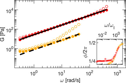
FIGURE 5. Amplitude G of the complex modulus G^∗ as obtained from frequency sweep measurement on glycerol (orange circles) and silicon oil (red circles). Empty (full) circles are obtained without (with) correction for inertia and friction. In the inset, we report the measured phase as a function of ω/ω_I without the correction. The lines are linear fits representing the expected (Newtonian) behavior.

We extract the viscosity of both samples by fitting a linear function of the experimental data after correction, which provides for glycerol (dashed line) and silicon oil (continuous line) viscosities equal to η = 0.86 ± 0.05 Pa⋅s and η = 26.6 ± 0.3 Pa⋅s, respectively. While the value for glycerol is in the range of expected values, also considering hydration [18, 19], the value for silicon oil is $\sim 10\%$ smaller than the one measured with a rheometer (Section 2.6), which we attribute to a comparable error in our estimate of the sample area due to meniscus formation after being loaded in the cell.

We report in Figure 6 results of frequency sweeps experiments with Sylgard (Figure 6A) and Carbopol 5% (Figure 6B). The experimental error bars, evaluated as the standard deviation of the mean over three different consecutive realizations, are typically smaller than the symbols, with the only exception of the loss modulus of Carbopol, due to an increasing uncertainty on the value of the phase. Lower precision in the phase determination mainly results from the increased duration of the experiments, which also increases the likelihood of an external perturbation of the system. Such an effect is less pronounced for Sylgard, whose large modulus makes it less sensitive to spurious perturbations and drifts. Overall, the storage and loss moduli for both samples can be measured over more than two decades in frequency, and are in agreement with rheology data obtained in Ref. [34] (Sylgard) and with our measurements with the rheometer (Carbopol 5%), as described in Section 2.6.

FIGURE 6

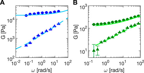
FIGURE 6. Storage (circles) and loss (triangles) moduli relative to (A) Sylgard (elastic sample) and (B) Carbopol 5% (yield stress sample) as a function of the oscillation frequency ω in oscillatory shear tests. Lines correspond to storage (continuous) and loss (dashed) moduli obtained with a commercial rheometer. Frequency sweeps are made at constant strain (1.5 ± 0.2% and 1.42 ± 0.09% for Sylgard and Carbopol, respectively). All data are corrected for inertia and sliding friction as described in the main text.

4.2 LAOS amplitude sweep

One of the most interesting applications of our setup lies in its capability to apply large amplitude oscillatory shears to a soft viscoelastic material, and simultaneously observe and characterize the rearrangements of suspended tracers within the sample.

The results of amplitude sweeps performed at different frequencies (ω = π, 2π and 4π rad/s) with Carbopol 5% are plotted in Figure 7, and show the expected behavior for a yield stress fluids: for small strain amplitudes (linear regime) the behavior is substantially elastic (i.e. the loss modulus is much smaller than the storage one) and the moduli are almost amplitude independent. Increasing the amplitude, we observe a progressive drop of G′, a peak in G″, and the crossover between G′ and G″. The crossover depends on the sampling frequency but is typically found for strain amplitudes between 80% and 100%. The fact that in our setup we observe an increase of G″ at the lowest probed strains is caused by the increasing contribution of sliding friction for decreasing values of the applied stress. In the SAOS regime, sliding friction effects are a consequence of our simplified treatment of friction, which sets a lower limit G″ ∼ σ_fr,0/γ₀ to frequency and amplitude sweeps. It is to be noted, however, that for a prescribed value of the sliding friction, such a limit can be pushed to lower values by increasing the sample area.

FIGURE 7

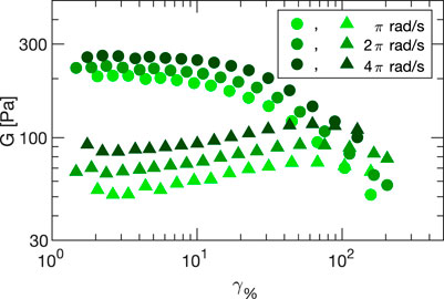
FIGURE 7. Storage (circles) and loss (triangles) moduli obtained from amplitude sweeps from the linear to the LAOS regime performed on Carbopol 5%. Different colors correspond to different angular frequencies ω equal to π rad/s (light green), 2π rad/s (green) and 4π rad/s (dark green). Error bars are smaller than the data points. All data are corrected for inertia and sliding friction as described in the main text.

It is important to stress that the values for G′ and G″ that we have obtained in LAOS tests originate from fitting the measured strain profile with a sinusoidal function. This procedure is the same used in commercial rheometers. From the temporal evolution of stress and strain within a period, we obtain Lissajous plots of stress as a function of the strain (Figure 8A) and of the strain rate (Figure 8B). To this aim, we first correct both the stage position and velocity for the drift contributions, which is done by subtracting from the raw data, the polynomial drift function $f_{\mathit{pol}}\left(t\right)$, and its analytical time derivative ${\dot{f}}_{\mathit{pol}}\left(t\right)$, respectively (see also Section 3.1). From the drift corrected position and velocity, the strain $\gamma \left(t\right)$ and the strain rate $\dot{\gamma }\left(t\right)$ are retrieved dividing by the gap. The average strain $\widehat{\gamma }\left(t\right)={\sum }_{n=0}^{N-1}\gamma \left(t+nT\right)$, with $t\in \left[0,T\right)$, is computed by averaging the strain over all the N measured periods. The average strain rate $\widehat{\dot{\gamma }}\left(t\right)$ is evaluated analogously.

FIGURE 8

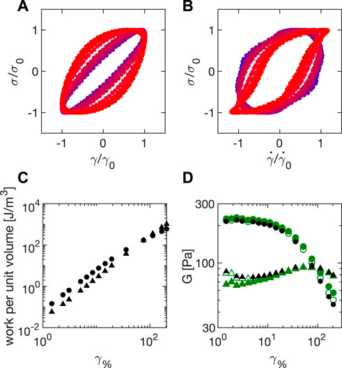
FIGURE 8. Amplitude sweeps for Carbopol 5% during LAOS at ω = 2π rad/s (A) Lissajous plot of the normalized stress $\sigma \left(t\right)$ versus the normalized strain $\gamma \left(t\right)$. Color scale progressively goes from low stresses (blue points, σ₀ = 3.5 Pa) to large stresses (red points, σ₀ = 190 Pa). (B) Lissajous plot of the normalized stress $\sigma \left(t\right)$ versus the normalized strain rate $\dot{\gamma }\left(t\right)$. Color scale is the same as in (A). (C) Dissipated energy per unit volume W_D (triangle) and elastic energy per unit volume W_E (circles) as obtained from the Lissajous plots in (A) and (B), respectively. (D) Storage (black circles) and loss (black triangles) moduli as obtained from the closed integral of the Lissajous plots. In green, we report the results obtained with a sinusoidal fit of $\gamma \left(t\right)$: full green symbols represent data corrected with inertia and sliding friction corrections and were already shown in Figure 7; both black and empty green symbols represent uncorrected data obtained from Lissajous integrals and from the fit, respectively.

To recover the temporal evolution of the stress, we divide the applied force by the measured area $\sigma \left(t\right)=F\left(t\right)/S$. Given the extreme precision of the SMU in supplying the signal, there is an extremely low discrepancy (average relative deviation ΔF/F < 4 ⋅ 10^–16) between consecutive measured periods of $F\left(t\right)$. We can therefore choose the first period of σ and, by assuming that it is virtually identical to the average over all the periods, identify the average stress $\widehat{\sigma }$ with it. Since the sampling frequency is different for force and displacement measurements, to recover Lissajous plots a direct association must be made between $\widehat{\sigma }$ on one side and $\widehat{\gamma }$ and $\widehat{\dot{\gamma }}$ on the other side. We perform this association by considering the discrete measurement times t of the strain and interpolating $\widehat{\sigma }$ at these times.

Combining all these steps, we obtain the Lissajous plots in Figures 8A,B, where we report for Carbopol 5% the values of $\widehat{\sigma }$, $\widehat{\gamma }$ and $\widehat{\dot{\gamma }}$ normalized with σ₀, γ₀, and ωγ₀. These plots reproduce the typical response for a yield stress fluid [35], with the stress-strain plot (8A) increasingly deviating from linearity and the stress-strain rate plot (8B) increasingly deviating from the initial elliptical shape, as the applied stress increases.

Beyond giving a very powerful visual representation of the rheological changes occurring within a material as the amplitude increases, the Lissajous plots in Figures 8A,B can be also used to extract quantitative information. In particular, the area under stress as a function of strain during a cycle quantifies the value of dissipated energy per unit volume [36]:

$W_D=\oint \widehat{\sigma }\left(\widehat{\gamma }\right)d\widehat{\gamma }.(14)$

Similarly, the elastic energy per unit volume is given by the area under stress as a function of strain during a cycle:

$W_E=\frac{1}{\omega }\oint \widehat{\sigma }\left(\widehat{\dot{\gamma }}\right)d\widehat{\dot{\gamma }}(15)$

These two quantities, calculated for Carbopol 5% at ω = 2π rad/s are shown in Figure 8C, where it appears immediately that a strain value can be identified beyond which the dissipated energy W_D overcomes the stored energy W_E. By definition, this value coincides with the crossover point between the moduli G′ and G″ (see Figure 7), which we can also estimate from the Lissajous analysis as

$G_{\mathit{liss}}^{\prime }=\frac{W_E}{\pi {\gamma }_0^2}(16)$

$G_{\mathit{liss}}^{″}=\frac{W_D}{\pi {\gamma }_0^2}.(17)$

The results obtained for the storage and loss moduli by using the Lissajous plots are reported in Figure 8D, where they are shown to agree with the results from the sinusoidal fit before operating the correction for inertia and friction, which is not implemented in the Lissajous plots. This agreement validates our different analyses.

In order to explore the microscopic counterpart of the yielding transition, we analyzed the shear-induced stroboscopic dynamics of embedded tracers for different strain amplitudes (Supplementary Movies SM2 and SM3). We first perform particle tracking analysis of the echo dynamics induced in the vorticity direction by shearing the sample Carbopol 5% at ω = 2π rad/s (amplitude sweep). In Figure 9A, we report the mean squared displacement (MSD) calculated (using 400 consecutive frames, and with 10 recorded points per period) for strain amplitudes 24.5% (blue), 105% (purple) and 188% (red). All the reported MSDs exhibit a linear behavior suggesting a diffusive-like behavior of the tracers that was previously observed in Ref. [11] with a similar Carbopol sample. The tracer mobility increases with the strain amplitude, but for small amplitudes exhibits an offset due to the tracking localization error. For this reason, we fitted the MSDs with a diffusive model accounting for the offset (dashed lines in the plot): MSD_v = σ_MSD + 2D_vΔt. The resulting D_v (inset of Figure 9) strongly depends on the strain amplitude, and spans over 4 orders of magnitude when the strain is increased by a factor of 10. Echo-DDM analysis of the same images (Figure 9B) provides q-dependent relaxation rates Γ(q) that are extracted by fitting the experimental ISFs to the model f (q, Δt) = exp (− Γ(q)Δt). The gray shadow corresponds to the region for which the estimation of the relaxation rates Γ(q) is not reliable since the relaxation times of f (q, Δt) for some wave vectors qs are longer than the acquisition time. By fitting the reliable points for the relaxation rate with a quadratic model Γ(q) = D_vq², which is typical for Brownian diffusion, we find a very good agreement between the diffusivity obtained by particle tracking and DDM, as shown in the inset. The agreement between PT and DDM is encouraging, as the former can be applied to investigate heterogeneous samples, whereas the latter is suited for small particles or for very dense non-index-matched complex fluids without recurring to tracers.

FIGURE 9

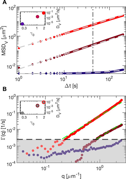
FIGURE 9. Microscopic, shear-induced dynamics of tracers embedded in Carbopol 5% shared at ω = 2π rad/s with strain amplitudes 24.5% (blue), 105% (purple) and 188% (red). (A) mean square displacement obtained from echo particle tracking analysis in the vorticity direction. Gray dashed lines are best fit with fitting function MSD_v = σ_MSD + 2D_vΔt. In the inset, we plot the diffusivity obtained from the fit as a function of the measured strain. (B) Relaxation rate from echo-DDM analysis of the same experiments. Green dashed lines are best fitting curves with the function Γ = D_vq². Gray shaded area identifies the region where fits are not reliable. In the inset, the diffusivity obtained from the fit (colored points) is compared with the one obtained from the PT analysis (gray points).

4.3 Triangular wave

During LAOS experiments one induces in the sample some microscopic, irreversible rearrangements that are larger for increasing strain amplitudes. While a sinusoidal perturbation of the sample is a simple, natural way to explore the frequency dependence of the sample mechanical properties, both strain and strain rates change during the period, thus making difficult the determination of the rearrangements dependence on these two parameters. A triangular wave, conversely, is characterized by a constant stress rate (unless a sign) while stress linearly changes in time. As a complementary oscillatory characterization, we therefore implemented the possibility to generate a triangular-wave stress with period 2π/ω₁ and amplitude σ₀ as

$\sigma \left(t\right)=\frac{2{\sigma }_0}{\pi }\arcsin \sin \left({\omega }_{1}t\right)(18)$

Although periodic, this function is not characterized by the single frequency ω₁ but by an infinite series of frequencies ω_n = nω₁ with n = 1, 3, … , ∞ according to its Fourier series

$\sigma \left(t\right)=\frac{8{\sigma }_0}{{\pi }^2}\sum _{n=\mathrm{1,3},\dots ,\infty }\frac{{\left(-1\right)}^{\left(n-1\right)/2}}{n^2}\sin {\omega }_{n}t.(19)$

Experimental normalized³ stress and strain profiles obtained during a triangular wave amplitude sweep with Carbopol 5% at ω₁ = 2π rad/s close to yielding (γ₀ = 68%), are reported in Figure 10A. While the applied stress is a neat triangular wave, the corresponding strain is shark-fin shaped. Indeed, the strain response to a triangular stress is expected to be triangular only in the linear regime.

FIGURE 10

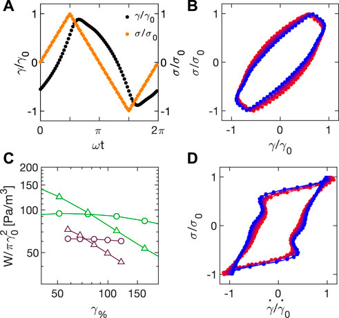
FIGURE 10. (A) Normalized stress σ/σ₀ (orange) and strain γ/γ₀ (black) during a triangular wave amplitude sweep at ω₁ = 2π rad/s. (B) Lissajous plot of the normalized stress σ/σ₀ as a function of the normalized strain γ/γ₀ relative to a triangular wave amplitude sweep at ω₁ = 2π rad/s. Colormap goes from blue to red as applied stress increases from 55 to 89 Pa. (C) Elastic (triangles) and dissipated (circles) energy normalized to $\pi {\gamma }_0^2$ as a function of the strain amplitude obtained for an amplitude sweep with a sinusoidal (green) and a triangular (purple) waveform. (D) Lissajous plot of the normalized stress σ/σ₀ as a function of the normalized strain rate $\dot{\gamma }/{\dot{\gamma }}_0$ relative to the same experiment of (B).

Information on the viscoelastic response for different stresses can be recovered from the analysis of the Lissajous plots, as described in Section 4.2. Triangular stresses as a function of strain and strain rate for different amplitudes are reported in Figures 10B,D, respectively. Of note, the stress-strain Lissajous evolves from a fairly defined rectangle to a more non-linear shape as stress increases (from blue to red). Also in this case, we can retrieve the elastic W_E and dissipated W_D energy from the circular integral of the data reported in Figures 10B,D, respectively. The results of this analysis for strains around the crossover are shown in Figure 10C (purple), after normalization with $\pi {\gamma }_0^2$. In contrast with the similar quantities obtained during a sinusoidal amplitude sweep (see Figure 8D and Figure 10C, green), here it is not correct to interpret $W/(\pi {\gamma }_0^2)$ as modulus, as they are defined as the response to a sinusoidal perturbation. However, the results obtained with the triangular wave exhibit a similar trend of the ones obtained with a sinusoidal perturbation, but the former are systematically smaller, as expected from the inequality

$\left|{\sigma }_0\sin \left({\omega }_{1}t\right)\right|\le \left|\frac{2{\sigma }_0}{\pi }\arcsin \sin \left({\omega }_{1}t\right)\right|.(20)$

Turning now to the local dynamics, we decided to compare in the same range of strains the results of echo PT analysis for both a triangular and a sinusoidal perturbation of Carbopol 5% across the yielding transition. We plot in Figure 11A the probability distribution of the displacements at time delay Δt = 43 s for the triangular (triangles) and the sinusoidal (squares) stress application. For both types of perturbation, distributions exhibits marked exponential tails. This combination of non-Gaussian statistics of the displacement and linear (Fickian) scaling of the MSD with time has been found to be a recurring feature of particles moving in heterogeneous environments [37, 38]. Remarkably, for the same measured strain amplitude (same color on the plot) distributions are sensibly larger for sinusoidal stress application. This picture is confirmed when the diffusion coefficients are extracted from PT analysis as a function of the strain amplitude (Figure 2B): shear-induced diffusion is less pronounced in the presence of triangular stresses compared to sinusoidal ones, suggesting that, at the same applied strain amplitude, shear-induced diffusion seems to correlate with the energy injected macroscopically per unit volume. The observed difference between the microscopic dynamics caused by triangular and sinusoidal stress profiles is particularly relevant from a methodological point of view, as it shows how being able to impose a variety of controlled stress profiles on the sample can be pivotal in connecting the microscopic dynamics with the macroscopic rheology of the sample. Future work will focus on other stress profiles, such as for instance chirped ones.

FIGURE 11

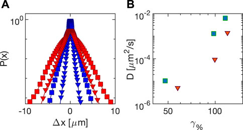
FIGURE 11. Echo particle tracking analysis of the dynamics of tracers in Carbopol 5% (A) Probability distribution for a time delay Δt = 43 s of the tracer displacements: squares (triangles) are obtained with sinusoidal (triangular) stress, whose amplitude is 98.6 ± 0.8% (blue) and 118 ± 2% (red). (B) Diffusion coefficients of the tracers as a function of strain amplitude for sinusoidal (squares) and triangular (triangles) stress profiles.

4.4 Creep and recovery

Creep and recovery tests have been performed with Sylgard and Carbopol, as prototypical elastic and viscoelastic materials, while simultanously studying the dynamics of embedded tracers. By switching on the magnet at t = 0 we create a sudden increase of the stress from zero to a value σ₀ (step-stress or creep). If a constant stress is applied to an elastic sample, the strain is expected to increase until reaching - after a transient - an equilibrium strain γ₀, from which the storage modulus can be recovered. As the applied stress return to zero (recovery phase), recovered strain can be measured as well, from which information on the dissipation can be derived [39].

In Figure 12A, we report the compliance J = γ/σ₀ measured during a creep and recovery experiment on a Sylgard sample with shear modulus 4.5 ⋅ 10⁴ Pa. The applied stresses span in a range of two decades from 53 to 8,300 Pa (inset of Figure 12A). The lower stress limit is set by the displacement detection: given the gap h = 332 μm, a strain of 0.1% corresponds in this measurement to a displacement of about 0.4 µm. This limit could be therefore in principle reduced by a factor 3 if the gap is increased to 1 mm. The upper limit, corresponding to a strain of 18%, comes from the high current intensity (1.3 A) necessary to reach the imposed stress of 8,300 Pa (area 1.4 ⋅ 10^–4 m²). These high currents are indeed close to the magnet loading limits. The purely elastic nature of Sylgard is confirmed both by the superposition of the compliances for all the values of applied stress, and by the complete recovery that is observed for long times. In the inset, the plateau strain obtained from an exponential fit of the creep part of $\gamma \left(t\right)$ is reported as a function of the applied stress. The superposed yellow dashed line is a linear fit from which the shear modulus G = 4.5 ⋅ 10⁴ Pa is recovered. Green points are the strain obtained from oscillatory experiments at three different σ₀ obtained with the same sample.

FIGURE 12

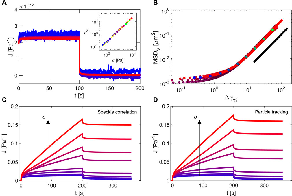
FIGURE 12. (A) Compliance measured in a series of creep and recovery experiments on a Sylgard sample with shear modulus 4.5 ⋅ 10⁴ Pa. Color scale ranges from the lower (blue) to the highest (red) applied stress, accordingly to the values reported on the abscissa of the inset, where the fitted strain creep plateau values are reported. In the inset, dashed white line is a linear fit of the plateau strains. Green points are the results obtained in oscillatory regime on the same sample. (B) MSD in the vorticity direction as a function of the strain, recovered from the four largest applied stresses of the dataset of C, on which it is possible to identify a constant strain rate on the time interval $\left[\mathrm{40,150}\right]$ s. The black line is a guide to the eye, representing a power law with exponent 1.4 (C) Macroscopic compliance measured from speckle correlation in a series of creep and recovery experiments with Carbopol 5%. Color scale ranges on the applied stresses ranging from σ = 4.7 Pa (blue) to σ = 51.8 Pa (red). (D) Local compliance measured from PT for the same experiment.

In Figure 12C, we show the compliances obtained from a series of creep and recovery experiments performed with Carbopol 5% for different imposed stresses. Carbopol flows for stress values around yielding, as for an imposed constant stress the strain does not approach a plateau value but linearly increases with time until stress holds. Lack of superposition of compliances for different stresses, even below yielding stress, and the lack of complete recovery testify the exit from the linear regime characterising lower stresses. Tracking the tracer particles as described in Section 3.2.3, we obtain the corresponding local compliance (Figure 12D), in excellent agreement with the global one in Figure 12C.

In the last analysis, we quantified the non-affine dynamics present when the system is flowing at a constant shear rate during creep tests. In Figure 12B we show the MSD in the vorticity direction corresponding to the four measurements with stresses close to yielding (28.2, 33.0, 37.7, and 51.8 Pa) as a function of the incremental strain $\mathrm{\Delta }\gamma =\mathrm{\Delta }t\dot{\gamma }$. The nice collapse of the curves suggests that non-affine dynamics depends only on strain and not on strain rate. This can be explained by the fact that, as in a typical yield stress material, the stress response for the probed strain rate values is constant. Conversely from what has been found in [40] for a jammed emulsion, the estimated MSD show superdiffusive scaling ∼ γ^1.4, which suggests that non-affine dynamics is directionally-persistent. However, a detailed discussion of this behaviour is beyond the scope of this study.

5 Conclusion

Here we describe a new rheo-microscopy setup that combines a stress-controlled rheometer with particle tracking and differential dynamic microscopy analysis of the motility of tracer particles. We tested the advantages and limitations of our setup with a variety of samples and tests, which were made possible by its versatility and flexibility. All the mechanical parts of the shear cell can easily be reproduced in any machine shop once having the technical drawings. All the remaining constitutive parts are commercially available, which makes the setup easily reproducible in any laboratory equipped with compressed air circuit. To further lower the barrier to implementation, we described in detail all the tests performed on the cell, the working principle of the acquisition protocol, and the data analysis algorithms.

A key feature of our setup is that it allows imaging of the entire sample height by means of long working distance objectives and optimized clear apertures. In such a way, by taking movies at different planes the cell allows extracting z-resolved information, which in turn provides a direct quantification of sample slip at the shear cell walls and makes it an excellent tool to investigate shear bending phenomena, thus allowing both a mesoscopic and a microscopic characterization of the deformation field. We believe that this capability will be of great help to settle important and long-standing issues, such as for instance the connection between shear banding and the microscopic structure and dynamics occurring within the banded material [27, 41, 42].

The wide range of accessible shearing frequencies, strain, and stresses allows for the exploration of both SAOS and LAOS regimes, with different types of periodic stress profiles, while simultaneously performing echo-imaging to separate non-affine displacements from affine ones and investigate shear-induced dynamics. Here we found evidence that, as the stress, and consequently the strain, increases during an amplitude sweep on a viscoelastic sample, shear-induced diffusion becomes faster (Section 4.2). By comparing different functional shapes of the applied periodic stress, we evidenced how such rearrangements are not only proportional to the amplitude of the strain the sample undergoes but depends on the energy absorbed and dissipated by the material during the whole shearing period (Section 4.3). Finally, we provide a different characterization by quantifying the local dynamics in non-periodic creep experiments, pointing out that non-affine dynamics is independent from the strain rate (Section 4.4).

Superposition rheology experiments could also be easily implemented, as well as comparative studies on the effect on sample properties of different pre-shearing procedures. The main limitation of the current design is the failure to operate when the applied stress is too small, a limit that can be easily overcome by increasing the sample area. Future perspectives foresee the possibility of also making strain-controlled experiments (with a feedback loop as in a commercial rheometer) and testing the cell with different imaging techniques, e.g. confocal microscopy.

Data availability statement

The raw data supporting the conclusion of this article will be made available by the authors, without undue reservation.

Author contributions

PE, VT, FG, and RC conceived the project and designed the experimental apparatus. SV assembled and tested the apparatus; SV and MB performed experiments; SV and MB analyzed the data. VT, FG, and RC coordinated the experimental activity. SV, MB, and RC wrote the first draft of the manuscript. All authors contributed to manuscript revision and read and approved the submitted version.

Funding

This work has been supported by: the Associazione Italiana per la Ricerca sul Cancro (AIRC) to FG and SV (MFAG#22083), the Swiss National Science Foundation (grant 172514) to VT.

Acknowledgments

The authors thank Stefano Aime and Giuliano Zanchetta for extensive and stimulating discussions. We thank IMCD Italia SpA for the kind gift of the Carbopol sample.

Conflict of interest

The authors declare that the research was conducted in the absence of any commercial or financial relationships that could be construed as a potential conflict of interest.

Publisher’s note

All claims expressed in this article are solely those of the authors and do not necessarily represent those of their affiliated organizations, or those of the publisher, the editors and the reviewers. Any product that may be evaluated in this article, or claim that may be made by its manufacturer, is not guaranteed or endorsed by the publisher.

Supplementary material

The Supplementary Material for this article can be found online at: https://www.frontiersin.org/articles/10.3389/fphy.2022.1013805/full#supplementary-material.

Footnotes

¹Commercial solutions such as the RheOptiCAD described in Ref. [10] can be used to investigate the microscopic dynamics under controlled shear strain conditions, as done for instance in Ref. [11]. However, the main limitation is that they do not provide a quantification of the stress, which makes them a “deformation tool” [10, 12, 13] rather than a rheometer. In addition, with this kind of cell one can usually apply only continuous shear or oscillatory shear deformations.

²https://github.com/dsseara/microrheology.

³Here, γ₀ is the strain amplitude evaluated from a fit of the measured strain with a triangular wave. Although the triangular wave fit is not optimal to reproduce the strain time evolution, it is suitable for a normalization whose sole purpose is to make data visualization more effective.

References

1. Besseling R, Isa L, Weeks ER, Poon WC. Quantitative imaging of colloidal flows. Adv Colloid Interf Sci (2009) 146:1–17. doi:10.1016/j.cis.2008.09.008

PubMed Abstract | CrossRef Full Text | Google Scholar

2. Dutta S, Mbi A, Arevalo RC, Blair DL. Development of a confocal rheometer for soft and biological materials. Rev scientific Instr (2013) 84:063702. doi:10.1063/1.4810015

PubMed Abstract | CrossRef Full Text | Google Scholar

3. Sentjabrskaja T, Chaudhuri P, Hermes M, Poon W, Horbach J, Egelhaaf S, et al. Creep and flow of glasses: Strain response linked to the spatial distribution of dynamical heterogeneities. Sci Rep (2015) 5:11884–11. doi:10.1038/srep11884

PubMed Abstract | CrossRef Full Text | Google Scholar

4. Koumakis N, Moghimi E, Besseling R, Poon WC, Brady JF, Petekidis G. Tuning colloidal gels by shear. Soft Matter (2015) 11:4640–8. doi:10.1039/c5sm00411j

PubMed Abstract | CrossRef Full Text | Google Scholar

5. Pommella A, Philippe AM, Phou T, Ramos L, Cipelletti L. Coupling space-resolved dynamic light scattering and rheometry to investigate heterogeneous flow and nonaffine dynamics in glassy and jammed soft matter. Phys Rev Appl (2019) 11:034073. doi:10.1103/physrevapplied.11.034073

CrossRef Full Text | Google Scholar

6. Chan HK, Mohraz A. A simple shear cell for the direct visualization of step-stress deformation in soft materials. Rheol Acta (2013) 52:383–94. doi:10.1007/s00397-013-0679-5

CrossRef Full Text | Google Scholar

7. Lin NY, McCoy JH, Cheng X, Leahy B, Israelachvili JN, Cohen I. A multi-axis confocal rheoscope for studying shear flow of structured fluids. Rev Scientific Instr (2014) 85:033905. doi:10.1063/1.4868688

PubMed Abstract | CrossRef Full Text | Google Scholar

8. Aime S, Ramos L, Fromental JM, Prevot G, Jelinek R, Cipelletti L. A stress-controlled shear cell for small-angle light scattering and microscopy. Rev Scientific Instr (2016) 87:123907. doi:10.1063/1.4972253

PubMed Abstract | CrossRef Full Text | Google Scholar

9. Singh A, Tateno M, Simon G, Vanel L, Leocmach M. Immersed cantilever apparatus for mechanics and microscopy. Meas Sci Technol (2021) 32:125603. doi:10.1088/1361-6501/ac1c1d

CrossRef Full Text | Google Scholar

10. Boitte JB, Vizcaïno C, Benyahia L, Herry JM, Michon C, Hayert M. A novel rheo-optical device for studying complex fluids in a double shear plate geometry. Rev Scientific Instr (2013) 84:013709. doi:10.1063/1.4774395

PubMed Abstract | CrossRef Full Text | Google Scholar

11. Edera P, Brizioli M, Zanchetta G, Petekidis G, Giavazzi F, Cerbino R. Deformation profiles and microscopic dynamics of complex fluids during oscillatory shear experiments. Soft Matter (2021) 17:8553–66. doi:10.1039/d1sm01068a

PubMed Abstract | CrossRef Full Text | Google Scholar

12. Shin S, Dorfman KD, Cheng X. Effect of edge disturbance on shear banding in polymeric solutions. J Rheology (2018) 62:1339–45. doi:10.1122/1.5042108

CrossRef Full Text | Google Scholar

13. Tu MQ, Lee M, Robertson-Anderson RM, Schroeder CM. Direct observation of ring polymer dynamics in the flow-gradient plane of shear flow. Macromolecules (2020) 53:9406–19. doi:10.1021/acs.macromol.0c01362

CrossRef Full Text | Google Scholar

14. Song J, Zhang Q, de Quesada F, Rizvi MH, Tracy JB, Ilavsky J, et al. Microscopic dynamics underlying the stress relaxation of arrested soft materials. Proc Natl Acad Sci U S A (2022) 119:e2201566119. doi:10.1073/pnas.2201566119

PubMed Abstract | CrossRef Full Text | Google Scholar

15. Pommella A, Cipelletti L, Ramos L. Role of normal stress in the creep dynamics and failure of a biopolymer gel. Phys Rev Lett (2020) 125:268006. doi:10.1103/physrevlett.125.268006

PubMed Abstract | CrossRef Full Text | Google Scholar

16. Cipelletti L, Martens K, Ramos L. Microscopic precursors of failure in soft matter. Soft matter (2020) 16:82–93. doi:10.1039/c9sm01730e

PubMed Abstract | CrossRef Full Text | Google Scholar

17. Dhont JK, Wagner NJ. Superposition rheology. Phys Rev E (2001) 63:021406. doi:10.1103/physreve.63.021406

PubMed Abstract | CrossRef Full Text | Google Scholar

18. Volk A, Kähler CJ. Density model for aqueous glycerol solutions. Exp Fluids (2018) 59:75–4. doi:10.1007/s00348-018-2527-y

CrossRef Full Text | Google Scholar

19. Grover D, Nicol J. The vapour pressure of glycerin solutions at twenty degrees. J Soc Chem Industry (1940) 59:175–7.

Google Scholar

20. Cerbino R. Quantitative optical microscopy of colloids: The legacy of jean perrin. Curr Opin Colloid Interf Sci (2018) 34:47–58. doi:10.1016/j.cocis.2018.03.003

CrossRef Full Text | Google Scholar

21. Crocker JC, Grier DG. Methods of digital video microscopy for colloidal studies. J Colloid Interf Sci (1996) 179:298–310. doi:10.1006/jcis.1996.0217

CrossRef Full Text | Google Scholar

22. Pelletier V, Gal N, Fournier P, Kilfoil ML. Microrheology of microtubule solutions and actin-microtubule composite networks. Phys Rev Lett (2009) 102:188303. doi:10.1103/PhysRevLett.102.188303

PubMed Abstract | CrossRef Full Text | Google Scholar

23. Adrian RJ. Scattering particle characteristics and their effect on pulsed laser measurements of fluid flow: Speckle velocimetry vs particle image velocimetry. Appl Opt (1984) 23:1690–1. doi:10.1364/ao.23.001690

PubMed Abstract | CrossRef Full Text | Google Scholar

24. Raffel M, Willert C, Wereley S, Kompenhans J. Particle image velocimetry. experimental fluid mechanics, 10. Berlin: Springer (2007). p. 978.

Google Scholar

25. Cerbino R, Trappe V. Differential dynamic microscopy: Probing wave vector dependent dynamics with a microscope. Phys Rev Lett (2008) 100:188102. doi:10.1103/physrevlett.100.188102

PubMed Abstract | CrossRef Full Text | Google Scholar

26. Giavazzi F, Brogioli D, Trappe V, Bellini T, Cerbino R. Scattering information obtained by optical microscopy: Differential dynamic microscopy and beyond. Phys Rev E (2009) 80:031403. doi:10.1103/physreve.80.031403

PubMed Abstract | CrossRef Full Text | Google Scholar

27. Divoux T, Fardin MA, Manneville S, Lerouge S. Shear banding of complex fluids. Annu Rev Fluid Mech (2016) 48:81–103. doi:10.1146/annurev-fluid-122414-034416

CrossRef Full Text | Google Scholar

28. Boukany PE, Wang SQ, Ravindranath S, Lee LJ. Shear banding in entangled polymers in the micron scale gap: A confocal-rheoscopic study. Soft Matter (2015) 11:8058–68. doi:10.1039/c5sm01429h

PubMed Abstract | CrossRef Full Text | Google Scholar

29. Pönisch W, Zaburdaev V. Relative distance between tracers as a measure of diffusivity within moving aggregates. Eur Phys J B (2018) 91:27–7. doi:10.1140/epjb/e2017-80347-5

CrossRef Full Text | Google Scholar

30. Giavazzi F, Edera P, Lu PJ, Cerbino R. Image windowing mitigates edge effects in differential dynamic microscopy. Eur Phys J E (2017) 40:97–9. doi:10.1140/epje/i2017-11587-3

PubMed Abstract | CrossRef Full Text | Google Scholar

31. Giavazzi F, Cerbino R. Digital Fourier microscopy for soft matter dynamics. J Opt (2014) 16:083001. doi:10.1088/2040-8978/16/8/083001

CrossRef Full Text | Google Scholar

32. Cerbino R, Piotti D, Buscaglia M, Giavazzi F. Dark field differential dynamic microscopy enables accurate characterization of the roto-translational dynamics of bacteria and colloidal clusters. J Phys : Condens Matter (2017) 30:025901. doi:10.1088/1361-648x/aa9bc5

PubMed Abstract | CrossRef Full Text | Google Scholar

33. Edera P, Bergamini D, Trappe V, Giavazzi F, Cerbino R. Differential dynamic microscopy microrheology of soft materials: A tracking-free determination of the frequency-dependent loss and storage moduli. Phys Rev Mater (2017) 1:073804. doi:10.1103/physrevmaterials.1.073804

CrossRef Full Text | Google Scholar

34. Prabowo F, Wing-Keung AL, Shen HH. Effect of curing temperature and cross-linker to pre-polymer ratio on the viscoelastic properties of a pdms elastomer. Adv Mat Res (2015) 1112:410–3. doi:10.4028/www.scientific.net/amr.1112.410

CrossRef Full Text | Google Scholar

35. Laurati M, Egelhaaf S, Petekidis G. Plastic rearrangements in colloidal gels investigated by Laos and ls-echo. J Rheology (2014) 58:1395–417. doi:10.1122/1.4872059

CrossRef Full Text | Google Scholar

36. Donley GJ, Singh PK, Shetty A, Rogers SA. Elucidating the G″ overshoot in soft materials with a yield transition via a time-resolved experimental strain decomposition. Proc Natl Acad Sci U S A (2020) 117:21945–52. doi:10.1073/pnas.2003869117

PubMed Abstract | CrossRef Full Text | Google Scholar

37. Wang B, Kuo J, Bae SC, Granick S. When brownian diffusion is not Gaussian. Nat Mater (2012) 11:481–5. doi:10.1038/nmat3308

PubMed Abstract | CrossRef Full Text | Google Scholar

38. Brizioli M, Sentjabrskaja T, Egelhaaf SU, Laurati M, Cerbino R, Giavazzi F. Reciprocal space study of brownian yet non-Gaussian diffusion of small tracers in a hard-sphere glass. Front Phys (2022) 10:408. doi:10.3389/fphy.2022.893777

CrossRef Full Text | Google Scholar

39. Calzolari D, Bischofberger I, Nazzani F, Trappe V. Interplay of coarsening, aging, and stress hardening impacting the creep behavior of a colloidal gel. J Rheology (2017) 61:817–31. doi:10.1122/1.4986465

CrossRef Full Text | Google Scholar

40. Vasisht VV, Dutta SK, Del Gado E, Blair DL. Rate dependence of elementary rearrangements and spatiotemporal correlations in the 3d flow of soft solids. Phys Rev Lett (2018) 120:018001. doi:10.1103/physrevlett.120.018001

PubMed Abstract | CrossRef Full Text | Google Scholar

41. Ozawa M, Berthier L, Biroli G, Rosso A, Tarjus G. Random critical point separates brittle and ductile yielding transitions in amorphous materials. Proc Natl Acad Sci U S A (2018) 115:6656–61. doi:10.1073/pnas.1806156115

PubMed Abstract | CrossRef Full Text | Google Scholar

42. Fielding SM. Shear banding in soft glassy materials. Rep Prog Phys (2014) 77:102601. doi:10.1088/0034-4885/77/10/102601

PubMed Abstract | CrossRef Full Text | Google Scholar