Vlasov simulation of the emissive plasma sheath with energy-dependent secondary emission coefficient and improved modeling for dielectric charging effects

A one-dimensional Vlasov–Poisson simulation code is employed to investigate the plasma sheath considering electron-induced secondary electron emission (SEE) and backscattering. The SEE coefficient is commonly treated as constant in a range of plasma simulations; here, an improved SEE model of a charged dielectric wall is constructed, which includes the wall charging effect on the SEE coefficient and the energy dependency of the SEE coefficient. Pertinent algorithms to implement the previously mentioned SEE model in plasma simulation are studied in detail. It is found that the SEE coefficient increases with the amount of negative wall charges, which in turn reduces the emissive sheath potential. With an energy-dependent SEE coefficient, the sheath potential is a nonlinear function of the plasma electron temperature, as opposed to the linear relation predicted by the classic emissive sheath theory. Simulation combining both wall-charging effect and SEE coefficient’ energy dependency suggests that the space-charged limited sheath is formed at high plasma electron temperature levels, where both sheath potential and surface charging saturate. Additionally, different algorithms to implement the backscattering in the kinetic simulation are tested and compared. Converting backscattered electrons to secondary electrons via an effective SEE coefficient barely affects the sheath properties. The simulation results are shown to be commensurate with the upgraded sheath theory predictions.

Introduction

A plasma sheath is a non-neutral space charge region that appears between bulk plasma and plasma-facing components. A sheath becomes emissive due to surface emission processes, including secondary electron emission (SEE), backscattering, field emission, thermionic emission, and photoemission. An emissive sheath widely appears in confined laboratory plasmas and plays a vital role in numerous industrial plasma applications such as plasma processing, electric proportion, plasma diagnostics, and plasma source [1–4]. The present research focuses on the algorithms to implement the interactions between plasma and dielectric surface in the kinetic simulation and the underlying sheath physics.

The classic emissive sheath theory was first established by Hobbs and Wesson by analyzing the current balance near a floating emissive boundary [5]. It was proved that the presheath structure is not significantly affected by boundary emission and the emissive sheath potential ${\phi }_{sh}$ is a function of the surface emission coefficient defined as ${\gamma }_e=\frac{{\Gamma }_{em}}{{\Gamma }_{ep}}$, with ${\Gamma }_{em}$, the surface emission flux and ${\Gamma }_{ep}$, the incoming plasma electron flux:

$e{\phi }_{sh}=T_e\ln \left[\left(1-{\gamma }_e\right)\sqrt{\frac{\mu }{2\pi }}\right].(1)$

Here, $T_e$ is the plasma electron temperature and $\mu =m_i/m_e$ is the ion–electron mass ratio. The study of the emissive sheath has been persistently developed since then, and a range of emissive sheath theories have been proposed [6–9]. For a strongly emissive surface, a space-charge limited (SCL) sheath with a nonmonotonic potential profile is formed when ${\gamma }_e$ exceeds a certain critical value [10]. More recent studies suggested that the SCL sheath cannot remain stable if cold ions are generated by charge exchange collisions in the sheath [11]. The emissive sheath is difficult to be directly accessed by conventional probe diagnostics due to its small size, so sheath theories are frequently validated against numerical simulations [12–14].

Common simulation approaches of plasma–surface interactions consist of a particle model, fluid model, kinetic model, and global model. The particle model provides self-consistent plasma dynamics based on first principles, which usually requires large quantities of computational resources. Fluid simulation is usually cheaper in terms of numerical cost, whereas one issue that potentially hinders the simulation accuracy is whether the fluid assumptions remain valid in the sheath region, particularly with non-thermal plasmas. Consequently, the sheath itself is frequently taken as a boundary condition instead of being simulated in the fluid model. The kinetic simulation captures the physics that are neglected in the fluid model when averaging over the velocity moments but exhibits lower performance when simulating complex reactions. In addition, the use of collision operators is inevitably less precise than the particle model. Yet one advantage of the kinetic simulation model is that it evades the statistical noise that must be reduced by using large macroparticle numbers in the particle model and provides smooth profiles for every time step. This benefit is particularly obvious for the nonlinear plasma behaviors in the sheath study. In addition, it is easier to directly control certain physical quantities to facilitate comparison with theory prediction in a kinetic model. This is why numerous kinetic models are employed in the study of sheath-related topics [15–18].

Boundary electron emission due to SEE is widely implemented in the numerical modeling of confined plasma. The SEE coefficient ${\gamma }_e$ depends on the incident electron energy and direction. SEE is, hence, intrinsically coupled with the plasma properties [19]. Additionally, the SEE coefficient is linked with the cumulative plasma fluxes, as the wall charges affect the extraction of excited internal secondary electrons (SEs) inside the material surface. Proper algorithms are therefore needed in order to implement these effects in the numerical simulation, which is the focus of the present work.

The article is structured as follows: Introduction introduces the employed simulation model; Introduction studies the methods to configure appropriate boundary conditions considering dielectric wall charges and the energy dependency of the SEE coefficient. The simulation setup involving electron backscattering is also expatiated. All simulation results are validated against upgraded emissive sheath theories, and the discrepancies between theory and simulation are analyzed.

Simulation setup

In this section, employed simulation algorithms and typical simulation results are presented. The simulation model is inspired by previous Vlasov–Poisson solvers [11, 15], and a basic version of the code was used in our recent simulations [13, 20, 21]. The employed 1D1V kinetic simulation code is based on the following kinetic equation:

$\frac{\partial f_s\left(x,v_s\right)}{\partial t}+v_s\frac{\partial f_s\left(x,v_s\right)}{\partial x}+\frac{q_{s}E\left(x\right)}{m_s}\frac{\partial f_s\left(x,v_s\right)}{\partial v_s}={\frac{\partial f_s\left(x,v_s\right)}{\partial t}|}_{coll}.(2)$

Here, the subscript s represents species; $m_s$, $q_s$, and $v_s$ are mass, charge, and velocity of the species; $E$ is the electric field; and the RHS is the collision source term. The code simulates the evolution of velocity distribution functions (VDFs) according to Eq 2. In the present work, only electrons and singly charged ions are considered. The electron and ion velocity distribution functions are initialized as uniformly distributed Maxwellian functions with temperatures $T_e$ and $T_i$ and density $n_0$:

$f_{s0}\left(x,v_s\right)=n_0\sqrt{\frac{m_s}{2\pi T_s}}\mathit{exp}\left(-\frac{m_s{v}_s^2}{2T_s}\right).(3)$

For the study of sheath properties, keeping a constant bulk plasma density facilitates the parameter scan. The collision term is separated into two parts: one plasma source term, which compensates for the boundary particle losses, and one relaxation term, which restores the plasma VDFs back to equilibrium at a constant rate (the BGK collision operator).

${\frac{\partial f_s\left(x,v_s\right)}{\partial t}|}_{coll}=S_{source}+{\nu }_s\left[\frac{n\left(x\right)}{n_0}{f}_{s0}-f_s\left(x,v_s\right)\right].(4)$

The collision frequency ${\upsilon }_s$ is set at being proportional to the inverse of the particle transit time, that is, ${\nu }_e\propto v_{eTh}/L$ and ${\nu }_i\propto v_{cs}/L$ with $v_{eTh}=\sqrt{\frac{T_e}{m_e}}$ being the electron thermal speed, $v_{cs}=\sqrt{\frac{T_e}{m_i}}$ being the sonic speed, and $L$ being the spatial range of the simulation domain. In the present simulation, ${\nu }_e=10v_{eTh}/L$ and ${\nu }_i=5v_{cs}/L$ are adopted. The coefficients are chosen to guarantee that the bulk plasma VDFs are not strongly diverged from the equilibrium. The charge source term is uniformly distributed in the region $\left(0.1L,0.9L\right)$, which equals to $S_{source}=1.25\frac{{\Gamma }_i}{n_{0}L}{f}_{s0}$, where ${\Gamma }_i$ is the total ion flux at two boundaries. The ion BGK relaxation is also turned on only in the region $\left(0.1L,0.9L\right)$. These two treatments avoid cold ion generation near the surface, such that a SCL sheath is not destroyed to form an inverse sheath. The present work mainly focuses on the classic Debye sheath. It should be noted that the ionization term here is simplified and does not consider realistic ionization collision, which aims at fixing the bulk plasma density at the desired level. A more physical collision operator was adopted in previous numerical modeling [22], where the ionization source is calculated by an integral of the ionization cross section, velocity, and background neutral density over EVDF. Such treatment provides more self-consistent simulation results where the ionization rate is closely coupled with the local EVDF. Implementing such a realistic collision operator in the present work will to some extent alter the bulk plasma properties, but the general validity of the obtained conclusions should be intact.

Boundary conditions of VDFs are critical for the implementation of the aforementioned surface processes. For a surface with only secondary electron emission, the emitted secondary electrons are assumed to follow a half-Maxwellian distribution with temperature $T_{em}$. Taking the left boundary as an example, the EVDF boundary condition is $f_{em}={f_e\left(v_e\right)|}_{x=0,v_e>0}=n_{em}\sqrt{\frac{2m_e}{\pi T_{em}}}\exp \left(-\frac{m_e{v}_e^2}{2T_{em}}\right)=C\exp \left(-\frac{m_e{v}_e^2}{2T_{em}}\right)$, where $n_{em}$ is the emitted electron density at the boundary. The factor $C$ is determined by the definition of the SEE coefficient, such that the emitted electron flux satisfies ${\Gamma }_{em}={\int }_0^{\infty }C\exp \left(-\frac{m_e{v}_e^2}{2T_{em}}\right)v_{e}d{v}_e={\gamma }_e{\Gamma }_{ep}$, with the plasma electron flux ${\Gamma }_{ep}=\left|{\int }_{-\infty }^0{f_e\left(v_e\right)|}_{x=0}d{v}_e\right|$ for the left boundary. Taking absolute value means that the flux is by default positive. The previously mentioned assumptions yield $f_{em}=\frac{m_e}{T_{em}}{\gamma }_e{\Gamma }_{ep}\exp \left(-\frac{m_e{v}_e^2}{2T_{em}}\right)$. This expression has been used in previous studies using the basic version of the adopted simulation code [20]. The boundary condition will be further reviewed in Simulation setup with improvements considering energy dependency and charging effects of the factor ${\gamma }_e$. Since no ion reflection is considered, the IVDF boundary condition is simply ${f_i\left(v_i\right)|}_{x=0,v_i>0}=0$ for the left boundary. The right boundary is symmetrical to the left in the present work.

A flow chart is given in Figure 1 to visualize the simulation procedure. For each time step, two advections are performed with an explicit finite difference method in the upwind scheme, and then the source term and BGK collision operator are applied. The velocity advection requires the electric field distribution, which is solved by assuming zero electric field in the center of the simulation domain and then integrating the net charge density toward the boundary using Gauss’s law. The simulation usually converges in several μs with a time step of 0.01 ns. The simulation convergence at $t=t_{end}$ is assumed to be achieved when parameters including sheath potential, wall charge density, and plasma flux at the wall all have small variations with a discrepancy lower than 0.1% in 10⁴ time steps. The time step is dictated by the Courant–Friedrichs–Lewy (CFL) stability criterion.

FIGURE 1

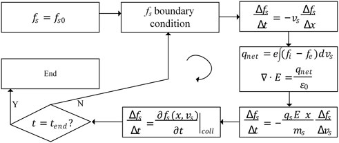
FIGURE 1. Schematic of the program execution.

Other choices of simulation parameters are introduced in the following sections. The plasma density is 5×10¹⁴ m⁻³, plasma electron temperature is 10 eV by default, ion temperature is 0.1 eV, emitted electron temperature is 2 eV, scale of simulation domain is 10 cm, spatial resolution is 10⁻⁴ m, and electron and ion velocity ranges cover eight times the electron thermal speed and sound speed, divided into 10³ points. Typical simulation results including potential, density, and velocity distribution functions with the aforementioned settings are shown in Figure 2.

FIGURE 2

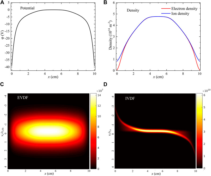
FIGURE 2. Typical simulation results obtained by the 1D1V kinetic simulation. (A) Space potential. (B) Electron and ion density. (C) Electron velocity distribution function. (D) Ion velocity distribution function.

Simulation results and model validation against theory

Influence of charge trapping on the SEE coefficient

A primary electron (PE) penetrating into a material surface, without being backscattered, generates internal secondary electrons while being slowed down. Only a fraction of the internal SEs is transported to the surface and escapes from the material, becoming true SEs. The transport of internal SEs is characterized by the escape mean free path ${\lambda }_{es}$, with the escape probability $P_{es}=\exp \left(-\frac{x}{{\lambda }_{es}}\right)$. The position $x$ is counted from where an SE is generated toward the material surface. Integrating $P_{es}$ multiplied by the generation function $g_{SE}$ over the whole range of PE’s trajectory, aka the primary range $R_p$, yields the SEE coefficient [23]:

${\gamma }_{e0}={\int }_0^{R_p}{g}_{SE}\left(x,{\epsilon }_{pe}\right)P_{es}\left(x\right)\mathrm{d}x.(5)$

The term ${\gamma }_{e0}$ represents the initial SEE coefficient for an uncharged wall when considering the charging effect, to be distinguished from ${\gamma }_e$ for a charged wall. By convention, the generation function is replaced by $1/{\lambda }_{SE}$ to facilitate derivation. The parameter ${\lambda }_{SE}$ is the mean free path of SE generation and has a dimension of a meter. Eq 5 is calculated as follows:

${\gamma }_{e0}=\frac{{\lambda }_{es}}{{\lambda }_{SE}}\left[1-\exp \left(-\frac{R_p}{{\lambda }_{es}}\right)\right]\approx \frac{{\lambda }_{es0}}{{\lambda }_{SE}},(6)$

supposing $R_p\gg {\lambda }_{es}$.

Eq 6 indicates that SEE is dictated by two characteristic lengths: ${\gamma }_{e0}=1$, if the mean free path to create a SE equals its escape mean free path; ${\gamma }_{e0}<1$, if SEs vanish quicker than their creation during the transport to the surface, and vice versa.

The value of ${\lambda }_{SE}$ is in general independent of the surface charging, and the surface charging mainly affects ${\gamma }_{e0}$ via the escape mean free path of SE, as internal SEs are captured by trap states or recombine with holes. These processes are prescribed by the density of the trap state and hole as well as the corresponding cross sections:

${\lambda }_{es0}^{-1}=N_T{\sigma }_T+N_h{\sigma }_R,(7)$

Here, $N_T$ and $N_h$ are intrinsic densities of trap states and holes and ${\sigma }_T$ and ${\sigma }_R$ are cross sections for trapping and recombination, respectively. For a classic Debye sheath, the plasma-facing wall is negatively charged, which means that some electron trap states are occupied. The escape mean free path of SE in a dielectric with trapped electron density $n_T$ (dimension m⁻³) is therefore expressed as

${\lambda }_{es}^{-1}=\left(N_T-n_T\right){\sigma }_T+N_h{\sigma }_R(8)$

with $n_T\le N_T$. Combining Eqs 6–8, the SEE coefficient with trapped charge is

${\gamma }_e=\frac{{\gamma }_{e0}}{1-{\lambda }_{es0}{n}_T{\sigma }_T}.(9)$

Eq 9 suggests that the dielectric surface immersed in a plasma becomes more emissive (larger ${\gamma }_e$) as negative surface charges accumulate. Note that this trend will not develop without limit, as higher surface emissivity decreases the amount of trapped charges, which in turn decreases ${\gamma }_e$. The increase of ${\gamma }_e$ also halts at the limit of $n_T=N_T$, which is, however, unlikely to be achieved for most laboratory plasmas. The sheath stability issue considering charge trapping will be addressed later in Influence of charge trapping on the SEE coefficient.

The term $n_T$, however, warrants more discussions before implementing surface charging effects in plasma simulation. The trapped charge density, to be distinguished from plasma density, represents the charges located in a layer much thinner than the plasma sheath. The surface layer of dielectric material, where trapped charges reside, is usually studied on a nanometer scale [24]. In the present simulation, the spatial grid resolution is 100 μm, which is well below the limit set by the Courant–Friedrichs–Lewy condition but is still above the nanometer scale by several orders of magnitude. It is, hence, difficult to simulate plasma coupled with a dielectric surface layer in real time. Therefore, Equation (9) is reformed as follows supposing all trapped charges are closely attached to the surface and an instantaneous charge transport process in the surface layer is assumed:

${\gamma }_e=\frac{{\gamma }_{e0}}{1-K_{wall}\left|{\sigma }_{wall}\right|}.(10)$

The wall-charging factor $K_{wall}$ is expressed as $K_{wall}={\lambda }_{es0}{\sigma }_T/\left(e{d}_{sl}\right)$, ${\sigma }_{wall}$ is the wall charge density (Cm⁻²), and $d_{sl}$ is the depth of the dielectric surface layer. The expression $n_T=\left|{\sigma }_{wall}\right|/e{d}_{sl}$ is used when deriving Eq 10. The updated ${\gamma }_e$ expression allows for facile implementation of the surface-charging effects in simulation models. The wall charge density is calculated by monitoring the surface electron and ion flux at each time step. The factor $K_{wall}$ is adjustable which contains all the necessary information about the charge transport process in the dielectric surface layer. ${\gamma }_{e0}$ is the uncharged SEE coefficient assigned at the beginning of the simulation.

A critical issue is then to determine the order of magnitude of the factor $K_{wall}$ for general applications of the aforementioned theories in plasma simulations. A rough estimation is given in the following sections based on classic SEE theories for solid materials. The most uncertain factor is the trapping cross section ${\sigma }_T$ as it varies strongly with the dielectric material, and the accurate theory prediction is in general difficult. From a range of experimental measurements [25–28], the trapping cross section is between 10⁻¹³–10⁻¹¹cm², but lower values exist. Here, to test the maximum effects of surface charging, the upper limit 10⁻¹¹cm² is taken. ${\lambda }_{es0}$ is calculated from ${\lambda }_{es0}={\lambda }_{SE}{\gamma }_{e0}$, with ${\lambda }_{SE}$ expressed by ${\lambda }_{SE}^{-1}=C\frac{1}{{\epsilon }_{ion}}\left|\frac{d{\epsilon }_{pe}\left(x\right)}{dx}\right|$. Here, $C\le 1$ and ${\epsilon }_{ion}$ are the mean excitation energy for one SE [29], approximated by ${\epsilon }_{ion}=3{\epsilon }_g+1eV$ [27], where ${\epsilon }_g$ is the gap energy of the dielectric material. $\frac{d{\epsilon }_{pe}\left(x\right)}{dx}$ is expressed using an empirical formula depending on the primary range and the primary electron current gradient [27]. Our calculation suggests that ${\lambda }_{es0}/d_{sl}$ is within the range of 10¹–10², which eventually gives $K_{wall}$ of 10⁵–10⁶ C⁻¹m². The aforementioned estimation is inevitably subjected to some levels of arbitrariness, and smaller values are possible since a peak ${\sigma }_T$ value is chosen here.

A range of ${\gamma }_{e0}$ values are assigned as initial conditions in the kinetic simulation, with different wall-charging factors $K_{wall}$, to study the effects of surface charging on emissive sheath properties. Other plasma parameters are kept constant. The charge trapping increases ${\gamma }_e$, which in turn reduces sheath potential and the amount of wall charges, shown in Figures 3A–C. Note that the charge conservation of a floating boundary requires that the amount of negative charges in the dielectric wall should be equal to the net positive charges in the sheath; hence, the sheath potential and wall charge density behave collectively. The value of ${\gamma }_{e,final}$ (${\gamma }_e$ value of a converged simulation run) scales up with $K_{wall}$, and cases with $K_{wall}=4\mathrm{E}6{\mathrm{C}}^{-1}{\mathrm{m}}^2$ exhibit a 35.5–87.2% improvement relative to the cases without charging effect in the selected range of ${\gamma }_{e0}$.

FIGURE 3

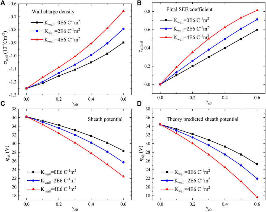
FIGURE 3. Emissive sheath properties with SEE considering the wall-charging effect, for a range of ${\gamma }_{e\mathit{0}}$ with different wall charging factors. (A) Wall charge density. (B) Final SEE coefficient after reaching convergence. (C) Sheath potential. (D) Sheath potential predicted by the emissive sheath theory.

Figure 3D shows the theoretical prediction of sheath potential according to Eqs. 1–10. Particularly, the black curve in Figure 3D is exactly the emissive sheath potential predicted by Hobbs, serving as a benchmark for code validity. Since the sheath potential in the simulation is counted from the wall to the central plasma, it includes both the sheath and presheath potential drop. A better way of presentation is to determine the presheath location from simulation and subtract it from the simulated total potential drop, but the determination of presheath incurs some uncertainties when analyzing simulation results, so the total potential drop is considered in the present work. The calculated emissive sheath potential from Equation (1) is, hence, augmented by $e^{0.5}{T}_e$ in Figure 3D, based on the Bohm presheath criterion. Same treatment is applied in the following sheath potential calculations. It should be noted that the Bohm presheath was proved not to be affected by the SEE [30]. It is clear that the simulation results and theoretical predictions agree considerably well. The discrepancies between Figures 3C,D are small when charging effects are not considered ($K_{wall}=0$), with a difference of 4.9–10.1% for the considered range of ${\gamma }_{e0}$. For cases considering charging effects, the peak discrepancy becomes 14.6 and 21.3% for $K_{wall}=2\mathrm{E}6{\mathrm{C}}^{-1}{\mathrm{m}}^2$ and $K_{wall}=4\mathrm{E}6{\mathrm{C}}^{-1}{\mathrm{m}}^2$, respectively. The discrepancies consist of the intrinsic discrepancy between simulation and theory without the charging effect, and the inconsistent choice of charge density when calculating ${\gamma }_e\left(n_T\right)$. The intrinsic discrepancy is likely related to the limited presheath region considered in the simulation. The discrepancy due to the charging effect is because the wall charge density should be self-consistently determined by the sheath potential, whereas the exact spatial potential profile is unknown from the emissive sheath theory. Since the theory-predicted sheath potentials are smaller than those predicted by the simulated results without charging effects, using larger wall charge densities from simulation (due to larger sheath potential) further increases the value of ${\gamma }_e$ and decreases the calculated sheath potential, leading to a larger discrepancy in the end.

Energy dependency of the SEE coefficient

In the Energy dependency of the SEE coefficient section, the SEE coefficient is kept constant for all incident electron energies. This is convenient for comparison with the classic emissive sheath theory (Eq 1) by Hobbs and Wesson [5] but is oversimplified as ${\gamma }_{e0}$ has a strong dependency on the incident electron energy ${\epsilon }_{PE}$ and angle ${\theta }_{PE}$. In the present 1D1V simulation, normal incidence is assumed. The SEE coefficient usually first increases with the primary electron energy up to a threshold energy level ${\epsilon }_{\mathit{max}}$ with peak value ${\gamma }_{max}$ and then begins to decrease. It should be noted that ${\epsilon }_{\mathit{max}}$ is in general several hundred eV and is therefore well above $T_e$ for most industrial plasmas and even fusion plasma in the scrape-off layer (SOL) near plasma-facing components. A typical SEE coefficient curve is shown in Figure 4, where primary electron energy and dimensionless SEE coefficient ${\gamma }_{e0}$ are normalized by two coefficients ${\epsilon }_{\mathit{max}}$ and ${\gamma }_{\mathit{max}}$. The following empirical formula is employed to derive the SEE coefficient curve [31]:

${\gamma }_{e0}\left({\epsilon }_{PE},{\theta }_{PE}\right)=1.526{\gamma }_{\mathit{max}}\left(1+\frac{k_s{\theta }_{PE}^2}{2\pi }\right)\left[1-\exp \left(-z^{1.725}\right)\right]/z^{0.725},(11)$

$z=1.284{\epsilon }_{PE}/\left[{\epsilon }_{\mathit{max}}\left(1+\frac{k_s{\theta }_{PE}^2}{\pi }\right)\right],(12)$

where the smoothness factor $k_s=1$ and incident angle ${\theta }_{PE}=0$ are applied and $z$ is also a dimensionless factor. In the energy range of industrial plasma electron, for example, below 100 eV, a linear approximation provides a good estimate of ${\gamma }_{e0}$, with ${\gamma }_{e0,estimat\mathrm{e}}\left(\epsilon \right)=\frac{\epsilon }{{\epsilon }_1}$. Here, ${\epsilon }_1$ is the required primary electron energy that produces one secondary electron. The values of ${\epsilon }_1$ are determined by setting ${\gamma }_{e0}=1$ in Eq 11. A comparison of linear approximation and real ${\gamma }_{e0}$ is shown in the subplot of Figure 4. A range of such empirical formulae exists which gives similar profiles of ${\gamma }_{e0}$ [19, 32].

FIGURE 4

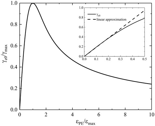
FIGURE 4. SEE coefficient as a function of incident electron energy. Normalization over ${\epsilon }_{\mathit{max}}$ and ${\gamma }_{\mathit{max}}$ is applied. The subplot shows the comparison of ${\gamma }_{e0}$ with its linear approximation in the low-energy range.

In boundary plasma simulations, the SEE coefficient is applied in a variety of ways depending on the employed simulation approach. For particle-in-cell (PIC) simulation, the implementation is straightforward, as ${\gamma }_{e0}$ of each super-particle is calculated individually by Eqs 11, 12. The decimal part of calculated ${\gamma }_{e0}$ is usually saved for the following super-particles until it cumulates up to one. For fluid simulation, the whole sheath region is commonly characterized by a boundary condition, for example, the sheath heat transmission coefficient, which constitutes the boundary condition of electric potential and heat flux, is sensitive to ${\gamma }_{e0}$. Since the sheath region is usually not simulated, the ${\gamma }_{e0}$ is calculated by ${\gamma }_{e0}\left(\langle {\epsilon }_{e,wall}\rangle \right)$, with $\langle {\epsilon }_{e,wall}\rangle$ being the estimated mean electron incident energy at the wall. For kinetic simulation, ${\gamma }_{e0}$ is better calculated by averaging ${\gamma }_{e0}$ over the EVDF at wall $f_{e,wall}$. Three different methods to apply SEE in the present simulation are tested, namely, 1) ${\gamma }_{e0}={\gamma }_{e0}\left(T_e/2\right)$ and ${\Gamma }_{em}={\gamma }_{e0}{\Gamma }_{ep}$, with $T_e/2$ obtained by integrating electron kinetic energy over Maxwellian EVDF; 2) ${\gamma }_{e0}={\gamma }_{e0}\left(\langle {\epsilon }_{e,wall}\rangle \right)$ and ${\Gamma }_{em}={\gamma }_{e0}{\Gamma }_{ep}$, with $\langle {\epsilon }_{e,wall}\rangle ={\int }_0^{\infty }0.5m_e{v}_e^2{f}_{pe,wall}dv/{\int }_0^{\infty }{f}_{e,wall}dv$; and 3) ${\Gamma }_{em}={\int }_0^{\infty }{\gamma }_{e0}\left(0.5m_e{v}_e^2\right)v_e{f}_{pe,wall}dv$, with the equivalent SEE coefficient ${\gamma }_{e0}={\Gamma }_{em}/{\Gamma }_{ep}$, ${\Gamma }_{ep}={\int }_0^{\infty }{v}_e{f}_{pe,wall}dv$. ${\gamma }_{e0}$ is updated at each time step for the last two methods. Scans of assigned plasma electron temperature in simulation $T_e$ are performed with two different (${\epsilon }_{\mathit{max}}$, ${\gamma }_{\mathit{max}}$) sets resembling typical dielectric wall materials, for the three approaches to implement the SEE coefficient. The obtained SEE coefficient and sheath potential are shown in Figure 5.

FIGURE 5

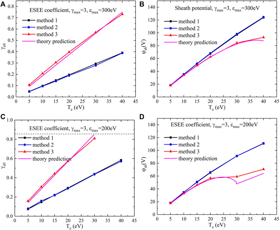
FIGURE 5. SEE coefficient and sheath potential calculated using three different ${\gamma }_{e0}$ setup methods obtained by simulation, in addition to the theory prediction. A series of plasma electron temperatures and two different (${\epsilon }_{\mathit{max}}$, ${\gamma }_{\mathit{max}}$) sets are applied. (A)–(B) ${\epsilon }_{\mathit{max}}=\mathit{300}eV$ and ${\gamma }_{\mathit{max}}=\mathit{3}$ and (C)–(D) ${\epsilon }_{\mathit{max}}=\mathit{200}eV$ and ${\gamma }_{\mathit{max}}=\mathit{3}$; (A), (C) show ${\gamma }_{e\mathit{0}}$, and (B), (D) show ${\phi }_{sh}$.

In order to verify the simulation results, the emissive sheath theory in Eq 1 is updated considering the energy dependency of ${\gamma }_{e0}$. In order to derive analytical sheath solution, the aforementioned approximation of the dimensionless SEE coefficient ${\gamma }_{e0}\left(\epsilon \right)=\frac{\epsilon }{{\epsilon }_1}$ is used. The effective SEE coefficient for plasma electron is calculated by

${\gamma }_{e0}=\frac{{\int }_0^{\infty }\frac{0.5m_e{v}_e^2}{{\epsilon }_1}{v}_e{f}_{pe,wall}dv}{{\int }_0^{\infty }{v}_e{f}_{pe,wall}dv}=\frac{T_e}{{\epsilon }_1}.(13)$

Hence, the sheath potential becomes

$e{\phi }_{sh}=T_e\ln \left[\left(1-\frac{T_e}{{\epsilon }_1}\right)\sqrt{\frac{\mu }{2\pi }}\right].(14)$

Eq 14 is only valid for the non-SCL sheath, which requires a SEE coefficient smaller than the critical value ${\gamma }_{e0}\le {\gamma }_{crit}\approx 1-8.3{\mu }^{-0.5}$ [5]. It should be noted that in the present article, all temperatures, ${\epsilon }_1$, and $e{\phi }_{sh}$ have the unit eV to facilitate calculation. The critical emission coefficient corresponds to a marginal sheath solution featuring zero electric field at the wall, with a critical sheath potential $e{\phi }_{sh,crit}\approx 1.02T_e$. The aforementioned analyses indicate that the plasma temperature should be lower than a critical temperature $T_{e,crit}$ to stay in the classic Debye sheath:

$T_e\le T_{e,crit}={\epsilon }_1\left(1-8.3{\mu }^{-0.5}\right).(15)$

In Figures 5A, B, the sheath remains in the classic sheath regime for the selected temperature range. The theory prediction is consistent with simulation results applied with the third method introduced previously. Simulations with methods 1 and 2 are close but in general underestimate ${\gamma }_{e0}$. Eq 14 suggests that ${\phi }_{sh}$ increases slower and even decreases as $T_e$ increases, as opposed to the classic emissive sheath theory which predicts a linear relation between sheath potential ${\phi }_{sh}$ and plasma electron temperature $T_e$. This trend is due to greater induced ${\gamma }_e$ with the increase in electron temperature, which is more obvious in Figures 5C, D, where ${\phi }_{sh}$ drops sharply to ${\phi }_{sh,crit}$ at approximately 30 eV. It should be noted that aforementioned expressions for ${\gamma }_{e0}$ are not valid when the sheath enters the SCL mode, as the formation of a local virtual cathode can reflect the emitted secondary electrons and also affect plasma electrons. The analytic formula of ${\gamma }_{e0}$ is difficult and is not given here but should not influence the sheath potential as it is no longer sensitive to ${\gamma }_{e0}$ above the critical emission yield. This is marked by a dashed line in Figure 5C, and also the linear dependence of sheath potential on $T_e$ is restored above 30 eV. The aforementioned trend is valid only for simulation with method 3 as the other two methods underestimate ${\gamma }_e$ so that ${\gamma }_{crit}$ is not achieved. The critical electron temperature is $T_{e,crit}=45.2eV$ for ${\epsilon }_{\mathit{max}}=300eV$ and ${\gamma }_{\mathit{max}}=3$ and is $29.8eV$ for ${\epsilon }_{\mathit{max}}=200eV$. This is because a smaller ${\epsilon }_{\mathit{max}}$ or larger ${\gamma }_{\mathit{max}}$ increases the slope of the left part of the SEE coefficient curve, which decreases ${\epsilon }_1$.

It should be noted that the adopted kinetic sheath theories mentioned previously are not valid when sheath collisionality becomes significantly higher, particularly when the ion-neutral collision mean free path is well below the Debye length. Ions are limited by their mobility at high pressure levels, and a clear presheath region cannot be defined. Fluid approaches are more favorable for the highly collisional sheath but will not be further developed in the present work.

In addition, it must be pointed out that the good agreement between kinetic sheath theory and the kinetic simulation results is partially due to the special choice of collision operator in the simulation, which ensures that the bulk plasma always follows the Maxwellian distribution at a given temperature. Larger discrepancies with the theories are expected for PIC simulation with more self-consistent treatment for collisions.

Combined SEE model and analyses of sheath stability

In the Combined SEE model and analyses of sheath stability section, the influences of wall charging and SEE coefficient energy dependency on sheath properties are discussed separately. The simulation results combining both factors are presented, applying method 3 for ${\gamma }_{e0}$ calculation introduced in Combined SEE model and analyses of sheath stability. The surface emission flux is calculated as

${\Gamma }_{em}={\int }_0^{\infty }\frac{{\gamma }_{e0}\left(0.5m_e{v}_e^2\right)}{1+K_{wall}{\sigma }_{wall}}{v}_e{f}_{pe,wall}dv(16)$

with ${\sigma }_{wall}\le 0$ and $f_{pe,wall}$ being the plasma electron VDF at the wall. Simulation results are shown in Figure 6. The theory prediction of SEE coefficient and sheath potential is calculated from Eqs, 10, 13, 14.

FIGURE 6

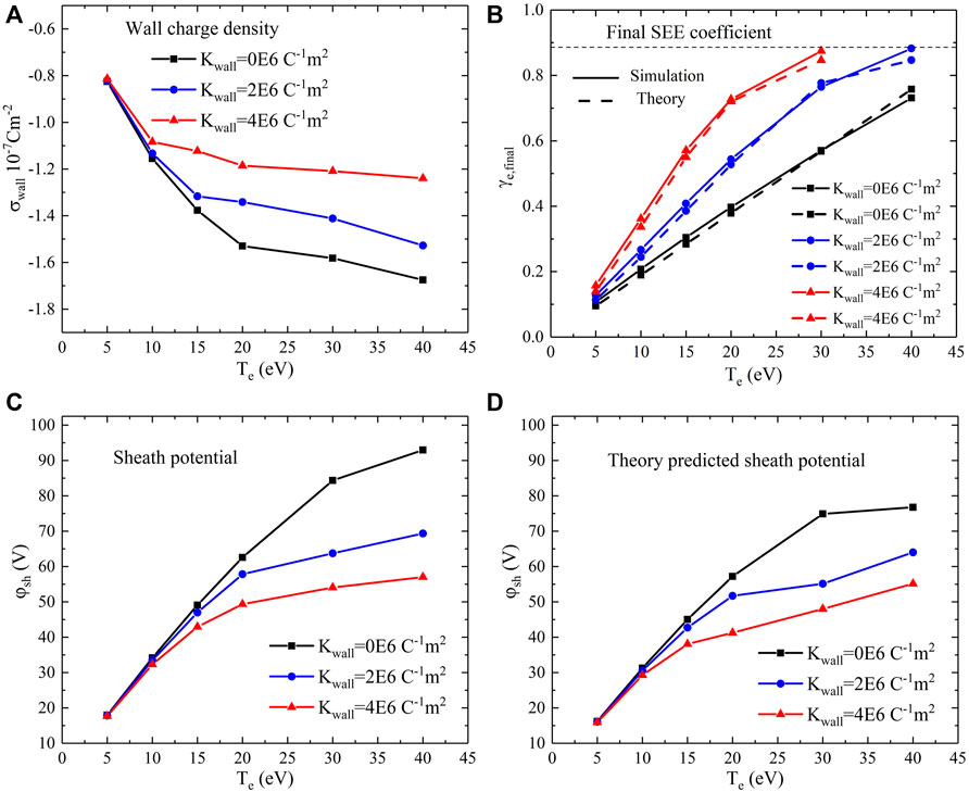
FIGURE 6. Emissive sheath properties with the combined SEE model, for a range of $T_e$ with different wall-charging factors. (A) Wall charge density. (B) Final SEE coefficient after reaching convergence; solid lines show simulation results, and dashed lines show theory prediction. (C) Sheath potential from simulation. (D) Sheath potential predicted by the emissive sheath theory.

The amount of wall charges increases with plasma electron temperature and decreases with the wall-charging factor $K_{wall}$, as shown in Figure 6A. Since both higher $T_e$ and $K_{wall}$ lead to higher SEE coefficient, ${\gamma }_e$ achieves the critical value marked by dashed lines at $K_{wall}=4E6C^{-1}{m}^2$ and $T_e\ge 30eV$, as shown in Figure 6B. Sheath potential given by the simulation and updated sheath theory shows a consistent trend with respect to $T_e$, which increases slowly at higher $T_e$ levels due to energy dependency of ${\gamma }_e$ and decreases with $K_{wall}$ due to wall charging.

One critical implication from the aforementioned analyses is whether the inclusion of charging effects and ${\gamma }_e$’s energy dependency will affect the I–V characterist of the sheath. The I–V characteristic of the emissive sheath is closely linked to the sheath stability and hence practical plasma applications. The sheath stability analyses considering both ${\gamma }_e$’s energy dependency and charging effects are analyzed as follows, which are based on previous emissive sheath stability studies assuming a constant SEE coefficient [33]. The net electron flux to the dielectric wall is ${\Gamma }_e={\Gamma }_{ep}-{\Gamma }_{em}=\left(1-{\gamma }_e\right){\Gamma }_{ep}$. Here, ${\gamma }_e$ depends on incident electron energy and the wall charge density. To guarantee a stable emissive sheath, the derivative $\frac{\partial {\Gamma }_e}{\partial {\phi }_{sh}}$ should be negative. A perturbation, for example, a small increase in ${\phi }_{sh}$, indicating that more negative charges are accumulated in the wall, must cause the net electron flux to decrease so that the sheath is restored back to equilibrium. The derivative $\frac{\partial {\Gamma }_e}{\partial {\phi }_{sh}}$ is further developed as

$\frac{\partial {\Gamma }_e}{\partial {\phi }_{sh}}=\left(1-{\gamma }_e\right)\frac{\partial {\Gamma }_{ep}}{\partial {\phi }_{sh}}-\frac{\partial {\gamma }_e}{\partial {\phi }_{sh}}{\Gamma }_{ep}<0.(17)$

Here, the sheath is assumed to be a classic Debye sheath with ${\gamma }_e<1$. The wall plasma electron flux is ${\Gamma }_{ep}={\Gamma }_{ep,se}\exp \left(-\frac{e{\phi }_{sh}}{T_{ep}}\right)$ with ${\Gamma }_{ep,se}$ being the plasma electron flux at the sheath edge. The first term in RHS of Eq 17 is, hence, negative. The derivative $\frac{\partial {\gamma }_e}{\partial {\phi }_{sh}}$ is further expressed as follows combining Eqs. 10, 13:

$\frac{\partial {\gamma }_{e0}}{\partial {\phi }_{sh}}=\frac{1}{1+K_{wall}{\sigma }_{wall}}\frac{1}{{\epsilon }_1}\frac{\partial T_e}{\partial {\phi }_{sh}}-\frac{K_{wall}}{{\left(1+K_{wall}{\sigma }_{wall}\right)}^2}\frac{T_e}{{\epsilon }_1}\frac{\partial {\sigma }_{wall}}{\partial {\phi }_{sh}}.(18)$

It should be noted that ${\sigma }_{wall}<0$ in the present analyses. If a constant plasma electron temperature is assumed, which is true for the present simulation but may vary in practical discharges, the RHS of Eq 18 should be positive since $\frac{\partial {\sigma }_{wall}}{\partial {\phi }_{sh}}<0$. This is because the amount of negative charges trapped in the wall is equal to the positive charge amount in the sheath, due to the charge conservation of a floating wall. A similar trend is also shown in Figures 3A,C, where ${\sigma }_{wall}$ and ${\phi }_{sh}$ change oppositely to ${\gamma }_e$. As a result, we consider that the charging effect does not alter the emissive sheath stability since the RHS of Eq 17 remains strictly negative. The conclusion is reassuring for applications such as plasma processing where stable plasma flux is expected.

Implementation of electron backscattering in simulation

In the aforementioned sections, the algorithms to implement secondary electron emission in the kinetic simulation are discussed in detail. Apart from SEE, some incident electrons on the solid wall are reflected back after elastic interactions with the sample atoms. Such process is called backscattering and in general occurs in a deeper region than that of SEE. The most distinct difference between the secondary electron and the backscattered electron is their velocity distribution functions. Backscattered electron velocity scales up with plasma electrons, whereas SEs mostly have low energy regardless of incident electron velocity.

A simple way to implement backscattering is to discard the different physical mechanisms of SEE and backscattering, assuming that both types of electrons have the same temperature and using an effective emission coefficient as follows [20]:

${\gamma }_{eff}=\left(1-R_b\right){\gamma }_e+R_b(19)$

with $R_b$ being the backscattering probability. The treatment simplifies the backscattering process as a special SEE with ${\gamma }_e=1$, whose implementation in both analytical analyses, and the simulation is straightforward by replacing ${\gamma }_e$ with ${\gamma }_{eff}$. The assumption adopted by Eq 19 is inevitably less accurate for high temperature electrons due to fast backscattered electrons. For kinetic simulation, more physical treatment is to use the following boundary condition for the EVDF:

${f_e\left(v_e\right)|}_{v_e>0,x=0}=\left(1-R_b\right)f_{em}+f_{eb}.(20)$

Here, $f_{eb}$ is the backscattered electron VDF. The separation of secondary electron and backscattered electron VDF is due to their different temperatures. The temperature of the secondary electron is fixed for the given wall material, while plasma electron temperature in practical discharge varies depending on particle and energy balances. If zero energy loss is assumed in the backscattering process, the reflected electron VDF is proportional to $f_{eb}\propto \exp \left(-\frac{m_e{v}_e^2}{2T_e}\right)$. Using the definition of the reflection coefficient ${\Gamma }_{ep}{R}_b={\Gamma }_b$ and backscattering flux ${\Gamma }_b={\int }_0^{\infty }{f}_{eb}{v}_{e}d{v}_e$, $f_{eb}$ is calculated as follows:

$f_{eb}=\frac{m_e}{T_e}{R}_b{\Gamma }_{ep}\exp \left(-\frac{m_e{v}_e^2}{2T_e}\right).(21)$

For the present simulation with Maxwellian plasma electron, Eq 20 is equivalent to

${f_e\left(v_e\right)|}_{v_e>0,x=0}=\left(1-R_b\right)f_{em}+R_b{f_e\left(v_e\right)|}_{v_e<0,x=0}.(22)$

Here, the left wall boundary is taken as an example, where the $v_e<0$ part of $f_e$ points to the left wall. In the adopted code, the aforementioned equation is implemented by setting $v_e>0$ part of $f_e$ at the left boundary to the sum of $\left(1-R_b\right)\frac{m_e}{T_{em}}{\gamma }_e{\Gamma }_{ep}\exp \left(-\frac{m_e{v}_e^2}{2T_{em}}\right)$ and $R_b$ times the $v_e<0$ part of $f_e$. ${\Gamma }_{ep}$ is obtained by integrating $v_e$ over $f_e$ (only for $v_e<0$), and ${\gamma }_e$ and $R_b$ are given as constant. The right wall boundary condition should be symmetrical.

The EVDFs at the left wall with two different boundary conditions mentioned previously are shown in Figure 7. It is clear that the boundary EVDFs using the two methods mentioned previously are remarkably different, mainly due to different emitted electron temperatures. Since the SEE-emitted electron temperature is typically within 5 eV whereas backscattered electrons have the same temperature as the plasma electrons, the discrepancy is obvious only for simulations with high $T_e$. The first method (Eq 19) usually yields an $f_{eb}$ more centralized than the second method (Eq 20).

FIGURE 7

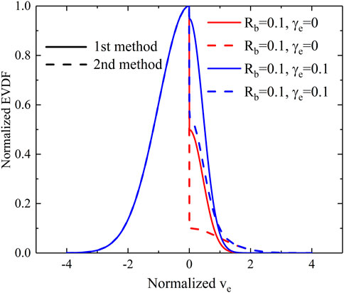
FIGURE 7. EVDF at the left wall with two different methods to set the boundary condition with backscattering.

The difference in boundary EVDF, however, is shown to have limited influences on simulation results, as shown in Figure 8. A scan of the true SEE coefficient with different backscattering coefficients is tested, with the effective SEE coefficient calculated as ${\gamma }_{eff}={\Gamma }_{em}/{\Gamma }_{ep}$. Here, ${\Gamma }_{em}$ contains contributions from both SEE and reflection. It should be noted that for low energy primary electrons, the reflection rate is unlikely to be very high and is typically below 0.2 [34]. The effective SEE coefficient calculated from simulation using Eq 20 is only slightly greater than the constant effective SEE coefficient prescribed by Eq 19. The sheath potentials are also almost equal accordingly. The conclusion is interesting as it suggests that the emissive sheath properties are not affected by using secondary electrons to replace backscattered electrons via a converting relation dictated by Eq 19, assuming that the incoming plasma electron flux is the same. Though having completely different physical mechanisms, the two types of electrons have similar contributions to the emissive plasma sheath properties. Adopting such an assumption will greatly simplify related theoretical works.

FIGURE 8

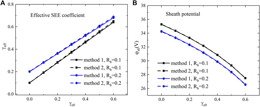
FIGURE 8. (A) Effective SEE coefficient and (B) sheath potential with a scan of true SEE coefficient and different backscattering coefficients.

With the aforementioned conclusions, the emissive sheath potential with both SEE and backscattering is simply

$e{\phi }_{sh}=T_e\ln \left[\left(1-\left(1-R_b\right){\gamma }_e-R_b\right)\sqrt{\frac{m_i}{2\pi m_e}}\right].(23)$

It should be noted that the conclusion mentioned previously is valid for purely elastic backscattering. If a constant fraction of energy $\eta =T_{eb}/T_{ep}$ is lost after the backscattering with $\eta$, the dimensionless backscattering energy loss factor and $T_{eb}$, the backscattered electron temperature, the predicted effective emission coefficient using Eq 19 is not affected, whereas the EVDF boundary condition in Eq 20 should be replaced by

${f_e\left(v_e\right)|}_{v_e>0,x=0}=\left(1-R_b\right)f_{em}+\frac{m_e}{\eta T_e}{R}_b{\Gamma }_{ep}\exp \left(-\frac{m_e{v}_e^2}{2\eta T_e}\right).(24)$

The influence of energy loss factor $\eta$ is shown in Figure 9. The factor $\eta$ is found to have a negligible influence on the sheath potential and effective SEE coefficient. The limited influence of emitted electron temperature on sheath properties is consistent with the emissive sheath theory, which predicts that the sheath potential depends only on the plasma electron temperature and effective SEE coefficient, instead of emitted electron temperature. The more recent kinetic theory considering truncated plasma electron VDF suggested that the influence of the ratio of plasma and emitted electron temperature $\Theta =T_e/T_{em}$ affects the sheath property, but the effect is obvious only when $T_e$ is close to $T_{em}$ [10], which is unlikely to be achieved here as the backscattered electron coefficient is low and effective temperature of all emitted electrons is close to $T_{em}$.

FIGURE 9

FIGURE 9. (A) Effective SEE coefficient and (B) sheath potential with a scan of backscattering coefficient using different η. The true SEE coefficient is kept as 0.1, and the theory prediction is given by Eq 23.

As has been pointed out in Implementation of electron backscattering in simulation, the use of artificial collision operator, though providing good agreement with the emissive sheath theory, can conceal certain physics that are only available in, for example, the PIC model where self-consistent plasma-neutral collisions are implemented. A comparison of the kinetic simulation and PIC simulation was recently performed for the capacitively coupled plasma subject to strong electron emission from the boundary [13, 35], where discrepancies are more obvious at high neutral pressure levels as the kinetic model does not implement realistic electron-neutral collisions and ionization sources. Similar comparisons between the kinetic and PIC models of the SEE coefficient charging effect are expected for DC or RF plasma conditions.

Conclusion

One-dimensional kinetic simulation of the plasma sheath is performed involving secondary electron emission and electron backscattering. The influence of accumulated wall charges on the SEE coefficient is considered and is shown to enhance the surface electron emission and decrease the sheath potential. Using an energy-dependent instead of static SEE coefficient is found to induce a nonlinear sheath potential response to the plasma electron temperature, as opposed to the classic emissive sheath theory. The SCL sheath is formed if plasma electron temperature or wall charge density is sufficiently high so that the effective SEE coefficient is above a critical value. The EVDF boundary condition for electron backscattering is proposed and implemented in the kinetic simulation. Considering backscattering electrons mainly affects boundary EVDF as backscattered electrons are typically faster than secondary electrons. Converting the backscattered rate into SEE coefficient via an equivalent equation is shown to barely affect the sheath properties. The simulation results are well supported by the upgraded emissive sheath theories, where wall-charging effect, SEE coefficient’s energy dependency, and backscattering are included.

Data availability statement

The raw data supporting the conclusion of this article will be made available by the authors, without undue reservation.

Author contributions

G-YS, B-HG, and SZ contributed to the concept of modeling and theory, and A-BS and G-JZ supervised the work throughout. All authors contributed to the final version of the manuscript.

Funding

The research was conducted under the auspices of the National Key R and D Program of China (No. 2020YFC2201100) and the National Natural Science Foundation of China (Nos. 51827809 and 52077169). This work was also supported in part by the Swiss National Science Foundation.

Conflict of interest

The authors declare that the research was conducted in the absence of any commercial or financial relationships that could be construed as a potential conflict of interest.

Publisher’s note

All claims expressed in this article are solely those of the authors and do not necessarily represent those of their affiliated organizations, or those of the publisher, the editors, and the reviewers. Any product that may be evaluated in this article, or claim that may be made by its manufacturer, is not guaranteed or endorsed by the publisher.

References

1. Zhang Y, Charles C, Boswell RW. Density measurements in low pressure, weakly magnetized, Rf plasmas: Experimental verification of the sheath expansion effect. Front Phys (2017) 2017:5. doi:10.3389/fphy.2017.00027

CrossRef Full Text | Google Scholar

2. Del Valle JI, Chang Diaz FR, Granados VH. Plasma-surface interactions within helicon plasma sources. Front Phys (2022) 2010:10. doi:10.3389/fphy.2022.856221

CrossRef Full Text | Google Scholar

3. Hershkowitz N. Sheaths: More complicated than you think. Phys Plasmas (2005) 12(5):055502. doi:10.1063/1.1887189

CrossRef Full Text | Google Scholar

4. Keidar M, Beilis I. Sheath and boundary conditions for plasma simulations of a Hall thruster discharge with magnetic lenses. Appl Phys Lett (2009) 94(19):191501. doi:10.1063/1.3132083

CrossRef Full Text | Google Scholar

5. Hobbs GD, Wesson JA. Heat flow through a Langmuir sheath in the presence of electron emission. Plasma Phys (1967) 9(1):85–7. doi:10.1088/0032-1028/9/1/410

CrossRef Full Text | Google Scholar

6. Anderson N. the formation of a plasma sheath with secondary electron emission. Int J Elect (1972) 32(4):425–33. doi:10.1080/00207217208938304

CrossRef Full Text | Google Scholar

7. Qing S, Wei J, Chen W, Tang S, Wang X. Stability of different plasma sheaths near a dielectric wall with secondary electron emission. J Plasma Phys (2019) 85(6):905850609. Epub 2019/12/04. doi:10.1017/S0022377819000862

CrossRef Full Text | Google Scholar

8. Ordonez CA, Peterkin RE. Secondary electron emission at anode, cathode, and floating plasma‐facing surfaces. J Appl Phys (1996) 79(5):2270–4. doi:10.1063/1.361151

CrossRef Full Text | Google Scholar

9. Zhonghua X, Xiaoyun Z, Feng W, Jinyuan L, Yue L, Ye G. Effect of secondary electron emission on the sheath in spt chamber. Plasma Sci Technol (2009) 11(1):57–61. doi:10.1088/1009-0630/11/1/12

CrossRef Full Text | Google Scholar

10. Sheehan JP, Hershkowitz N, Kaganovich ID, Wang H, Raitses Y, Barnat EV, et al. Kinetic theory of plasma sheaths surrounding electron-emitting surfaces. Phys Rev Lett (2013) 111(7):075002. doi:10.1103/PhysRevLett.111.075002

PubMed Abstract | CrossRef Full Text | Google Scholar

11. Campanell MD, Umansky MV. Strongly emitting surfaces unable to float below plasma potential. Phys Rev Lett (2016) 116(8):085003. doi:10.1103/PhysRevLett.116.085003

PubMed Abstract | CrossRef Full Text | Google Scholar

12. Taccogna F. Non-classical plasma sheaths: Space-Charge-Limited and inverse regimes under strong emission from surfaces. Eur Phys J D (2014) 68(7):199. doi:10.1140/epjd/e2014-50132-5

CrossRef Full Text | Google Scholar

13. Sun G-Y, Sun A-B, Zhang G-J. Intense boundary emission destroys normal radio-frequency plasma sheath. Phys Rev E (2020) 101(3):033203. doi:10.1103/PhysRevE.101.033203

PubMed Abstract | CrossRef Full Text | Google Scholar

14. Zhang Z, Wu B, Yang S, Zhang Y, Chen D, Fan M, et al. formation of stable inverse sheath in ion–ion plasma by strong negative ion emission. Plasma Sourc Sci Technol (2018) 27(6):06LT1. doi:10.1088/1361-6595/aac070

CrossRef Full Text | Google Scholar

15. Coulette D, Manfredi G. An eulerian Vlasov code for plasma-wall interactions. J Phys : Conf Ser (2014) 561:012005. doi:10.1088/1742-6596/561/1/012005

CrossRef Full Text | Google Scholar

16. Cagas P, Hakim A, Juno J, Srinivasan B. Continuum kinetic and multi-fluid simulations of classical sheaths. Phys Plasmas (2017) 24(2):022118. doi:10.1063/1.4976544

CrossRef Full Text | Google Scholar

17. Juno J, Hakim A, TenBarge J, Shi E, Dorland W. Discontinuous galerkin algorithms for fully kinetic plasmas. J Comput Phys (2018) 353:110–47. doi:10.1016/j.jcp.2017.10.009

CrossRef Full Text | Google Scholar

18. Campanell MD, Johnson GR. Thermionic cooling of the target plasma to a sub-ev temperature. Phys Rev Lett (2019) 122(1):015003. doi:10.1103/PhysRevLett.122.015003

PubMed Abstract | CrossRef Full Text | Google Scholar

19. Vaughan JRM. A new formula for secondary emission yield. IEEE Trans Electron Devices (1989) 36(9):1963–7. doi:10.1109/16.34278

CrossRef Full Text | Google Scholar

20. Sun G-Y, Li Y, Zhang S, Song B-P, Mu H-B, Guo B-H, et al. Integrated modeling of plasma-dielectric interaction: Kinetic boundary effects. Plasma Sourc Sci Technol (2019) 28(5):055001. doi:10.1088/1361-6595/ab17a3

CrossRef Full Text | Google Scholar

21. Sun G-Y, Li H-W, Sun A-B, Li Y, Song B-P, Mu H-B, et al. On the role of secondary electron emission in capacitively coupled radio‐frequency plasma sheath: A theoretical ground. Plasma Process Polym (2019) 16(11):1900093. doi:10.1002/ppap.201900093

CrossRef Full Text | Google Scholar

22. Levko D, Arslanbekov RR, Kolobov VI. Modified paschen curves for pulsed breakdown. Phys Plasmas (2019) 26(6):064502. doi:10.1063/1.5108732

CrossRef Full Text | Google Scholar

23. Lye RG, Dekker AJ. Theory of secondary emission. Phys Rev (1957) 107(4):977–81. doi:10.1103/PhysRev.107.977

CrossRef Full Text | Google Scholar

24. Heinisch RL, Bronold FX, Fehske H. Electron surface layer at the interface of a plasma and a dielectric wall. Phys Rev B (2012) 85(7):075323. doi:10.1103/PhysRevB.85.075323

CrossRef Full Text | Google Scholar

25. Zhao CZ, Zhang JF, Zahid MB, Govoreanu B, Groeseneken G, De Gendt S. Determination of capture cross sections for as-grown electron traps in Hfo2∕Hfsio stacks. J Appl Phys (2006) 100(9):093716. doi:10.1063/1.2364043

CrossRef Full Text | Google Scholar

26. Boughariou A, Damamme G, Kallel A. Evaluation of the effective cross-sections for recombination and trapping in the case of pure spinel. J Microsc (2015) 257(3):201–7. doi:10.1111/jmi.12202

PubMed Abstract | CrossRef Full Text | Google Scholar

27. Ghorbel N, Kallel A, Damamme G. Analytical model of secondary electron emission yield in electron beam irradiated insulators. Micron (2018) 112:35–41. doi:10.1016/j.micron.2018.06.002

PubMed Abstract | CrossRef Full Text | Google Scholar

28. Belhaj M, Odof S, Msellak K, Jbara O. Time-dependent measurement of the trapped charge in electron irradiated insulators: Application to Al2o3–sapphire. J Appl Phys (2000) 88(5):2289–94. doi:10.1063/1.1287131

CrossRef Full Text | Google Scholar

29. Fitting H-J, Glaefeke H, Wild W. Electron penetration and energy transfer in solid targets. Phys Stat Sol (1977) 43(1):185–90. doi:10.1002/pssa.2210430119

CrossRef Full Text | Google Scholar

30. Kaganovich ID, Raitses Y, Sydorenko D, Smolyakov A. Kinetic effects in a Hall thruster discharge. Phys Plasmas (2007) 14(5):057104. doi:10.1063/1.2709865

CrossRef Full Text | Google Scholar

31. Sun G-Y, Guo B-H, Mu H-B, Song B-P, Zhou R-D, Zhang S, et al. Flashover strength improvement and multipactor suppression in vacuum using surface charge pre-conditioning on insulator. J Appl Phys (2018) 124(13):134102. doi:10.1063/1.5048063

CrossRef Full Text | Google Scholar

32. Schwarz SA. Application of a semi‐empirical sputtering model to secondary electron emission. J Appl Phys (1990) 68(5):2382–91. doi:10.1063/1.346496

CrossRef Full Text | Google Scholar

33. Sydorenko D, Smolyakov A, Kaganovich I, Raitses Y. Plasma-sheath instability in Hall thrusters due to periodic modulation of the energy of secondary electrons in cyclotron motion. Phys Plasmas (2008) 15(5):053506. doi:10.1063/1.2918333

CrossRef Full Text | Google Scholar

34. Hussain A, Yang L, Mao S, Da B, Tőkési K, Ding ZJ. Determination of electron backscattering coefficient of beryllium by a high-precision Monte Carlo simulation. Nucl Mater Energ (2021) 26:100862. doi:10.1016/j.nme.2020.100862

CrossRef Full Text | Google Scholar

35. Zhang S, Sun G-Y, Chen J, Sun H-M, Sun A-B, Zhang G-J. On the ohmic-dominant heating mode of capacitively coupled plasma inverted by boundary electron emission. Appl Phys Lett (2022) 121(1):014101. doi:10.1063/5.0096316

CrossRef Full Text | Google Scholar