Accuracy Enhancement of LIBS-XRF Coal Quality Analysis Through Spectral Intensity Correction and Piecewise Modeling

The combination of laser-induced breakdown spectroscopy and energy dispersive X-ray fluorescence spectroscopy in the coal quality analysis was reported formerly. But in the practical test of the prototype instrument in the real power plant, the X-ray fluorescence signals suffered from intensity fluctuations over long-time measurements. The long-term signal fluctuations cause lower efficiency on the establishment of the calibration model and relatively larger root-mean-squared error of prediction (RMSEP) for unknown samples. Therefore, the spectral intensity correction was performed in the measurements; a randomly selected sample was measured several times in the whole measurements, including the modeling samples and unknown samples, recording the signal fluctuations and searching for a set of factors suitable for the intensity correction of a full-spectrum–based partial least square calibration model. In addition, as the signals of the coal samples of the power plant showed the potential of classification, the piecewise models were also established in case of further enhancement of the model or prediction accuracy. The RMSEPs of the calorific value, ash, volatile, and sulfur were lowered from 0.68 MJ/kg, 1.62%, 0.32%, and 0.24% to 0.51 MJ/kg, 1.34%, 0.16%, and 0.14% after spectral intensity correction, respectively. The piecewise modeling with spectral intensity correction achieved similar RMSEP for volatile and sulfur prediction but with more accurate models. The spectral intensity correction showed the ability to reduce the long-term signal fluctuation, and piecewise modeling also showed more efficiency in the model establishments for volatile and ash determination.

1 Introduction

Coal is still the major source of electric power in China. As an increasing attention toward environmental problems, clean, highly efficient, and intelligent coal-fired power plants are expected, which could act more modernized and have less pollution. For a coal-fired power plant, the quality control of purchased coal is an important part for its economic and clean operation. The current coal quality analysis in the coal-fired power plants of China relies on several chemical analyzers developed based on the Chinese national standards of coal quality analysis (GB/T 30732-2014, GB/T 213-2008, GB/T 214-2007), which require 40–60 min in total for the measurements of calorific value, ash, volatile, and sulfur for a single sample. The real-time coal quality control and pricing are impossible in this way. Therefore, a single-instrument fast coal quality analyzer is valuable for such coal-fired power plants.

Laser-induced breakdown spectroscopy (LIBS) is a promising technique for elemental analysis. Its advantages of high analytical speed, low cost, simultaneous multi-elemental capacity, in-situ, and real-time analysis ability make it suitable for a wide field of applications, such as space exploration [1], environmental monitoring [2], energy [3], biomedicine [4], and other fields [5–8]. The use of LIBS in coal quality analysis has also been studied for several years. Zhang et al. studied the determination of the organic oxygen content with LIBS. A calibration model of 1.15–1.37% in accuracy was established [9]. Yin et al. designed a LIBS system for online pulverized coal quality analysis in the power plant, which achieved elemental measurement errors within 10% and ash measurement error in the range of 2.29–13.47% [10]. Chen et al. studied the moisture content influences in the LIBS measurement of coal [11]. Yu et al. studied the difference of the matrix effect when measuring particle or pellet coal sample with LIBS [12]. Jie et al., Li et al., Hou et al., and Zhang et al. developed or tried multiple calibration methods to improve the prediction ability and repeatability of LIBS coal analysis, including special spectrum standardization, partial least square (PLS) regression, support vector machine regression, artificial neural network, and principal component regression [13–16]. Despite the advantages of the LIBS analysis, this technique still suffers from less measurement repeatability and matrix effect, limiting its performance for practical use.

X-ray fluorescence (XRF) spectroscopy also offers multi-elemental analysis ability and has been studied on the multi-elemental determination of coal samples. Li et al. utilized the high-pressure pressed powder pellet technique for wavelength dispersive XRF (WDXRF) to improve the sensitivity and precision of the coal component analysis [17]. Their results showed increased repeatability when using high pressure. Compared with WDXRF, the energy-dispersive XRF (EDXRF) can be simpler in structure and of low cost. Besides, the power of X-ray can be much lower for radiation safety. Wawrzonek and Parus tried multivariate linear regression with elemental lines of XRF to determine the ash content in coal [18]. Ma utilized the EDXRF instrument to evaluate the measurements of Si, Al, Fe, Ca, Mg, Ti, K, Na, and P contents in coal ash [19]. XRF provides more stable signals than LIBS, which guarantees better repeatability of the analytical results. However, for EDXRF, the detection of signals for light elements such as Na and Mg is poor, and analyses of C and H are virtually impossible, which limit its use in coal quality analysis.

Therefore, a solution of LIBS combined with EDXRF was proposed [20] to make use of the advantages of both techniques. Then, the prototype of the LIBS-XRF instrument was developed and tested in the coal-fired power plant of Shanxi Yangguang Power Generation Co., Ltd. The PLS algorithm was used to establish the calibration models. In order to take the best advantage of the repeatability of XRF signals, the input data of the PLS model consisted of continuous XRF spectral signals covering all peaks and the integral intensities of C, Na, and H lines from the LIBS signal. However, different from laboratory conditions, long-term fluctuations of XRF signals appeared in the measurements in the power plant, which reduced the prediction accuracy of the results. As a consequence, a random selected sample, treated as a standard sample, was measured by XRF several times in the whole measurement procedure of the coal samples in the power plant for both illustrating the signal fluctuations and correcting the fluctuations of the input data for the model establishment and prediction. On the other hand, piecewise modeling was possible based on the large sample volume, expecting to improve modeling precision. In this article, the spectral intensity correction based on repeated measurements of the standard sample and the piecewise modeling method is discussed for increasing the accuracy of the LIBS-XRF coal quality analysis instrument. The performances were assessed by the root-mean-squared error (RMSE) and the determination coefficient (R²) of the calibration models, together with the RMSE of prediction (RMSEP) results. Relatively small RMSEPs are expected for the power plant, which are related to the tiered pricing of coal (GB/T 7562-2018).

2 Experimental

2.1 Experimental Setup

Figure 1 illustrates the principle of the LIBS-XRF instrument. It consists of the XRF measurement part, LIBS measurement part, and sample transport part. The XRF measurement part is a self-designed EDXRF system. The rhodium anode sealed X-ray tube operates at 10 kV/0.25 mA, and the XRF signal is collected by a silicon drift detector (SDD). The magnification of the SDD is set at a value that the nonzero XRF signal covers the 4,096 channels properly. The X-ray incidence and collection paths are sealed for the vacuum-operating environment of 100–200 Pa, and there is a slim beryllium window in the X-ray path above the sample surface for the X-rays to pass through. The LIBS measurement part utilizes a diode-pumped Q-switched Nd:YAG laser (M-NANO-Nd:YAG-8ns-60-LPCEI_PR139C3, Montfort Laser) for excitation, operating at 1,064 nm, 8 ns, 6 Hz, and 60 mJ per pulse. The laser pulse is focused slightly below the sample surface using a flat convex lens with a focal length of 100 mm. The LIBS signal is collected from the side of the plasma by an optical fiber into a dual-channel spectrometer (AvaSpec-ULS4096CL-EVO, 195–321 and 497–732 nm, Avantes), and the spectral resolution is 0.09–0.11 nm for channel 1 and 0.18–0.18 nm for channel 2. The integral time of the spectrometer is 1 ms. In the sample transport part, the translation stage is controlled by programmable logical controller (PLC) to hold and transport the sample for XRF measurement of 60 s first and then for LIBS measurement of 300 pulses, and the sample is rotated during the whole measurement. The whole control and data processing are operated by using a computer.

FIGURE 1

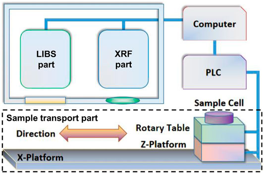
FIGURE 1. Scheme of the LIBS-XRF instrument.

2.2 Sample Preparation and Grouping

The coal samples in this test were provided by the chemical laboratory of the power plant. These samples were originally collected from the coal-carrying haulage trucks. The collected samples were then milled into powders less than 200 μm in size and dried during the measurement of moisture in advance. Before being measured by the LIBS-XRF instrument, the powdered sample must be prepared into pellets. The samples were expected to be pressed directly into pellets, 32 mm in diameter with 20 tons of pressure holding for 20 s. Due to the poor self-binding property of the dry anthracite coal powders in the laboratory, there was a 50% risk of failure for the direct pressing strategy, affecting the operating efficiency of the whole measurement procedure. To avoid the risk of sample preparation failure, the strategy of sample preparation was then changed; for XRF measurement, the coal powders were filled in a holder and the sample surface was flattened, and as for LIBS measurement, KBr was added as a binder into the coal powders with a volume proportion of 6:1 and then the mixture was pressed into pellets as expected.

The coal property values, including calorific value, ash, volatile, and sulfur, were obtained directly from the chemical measurement results of the chemical laboratory in the power plant. The ranges of these values for the coal samples establishing the calibration model were 16.99–30.88 MJ/kg, 12.24–47.84%, 5.36–11.16%, and 1.21–3.79%, respectively.

There were 316 individual samples measured eventually for establishing the calibration models. Besides, another seven samples were measured for evaluating the performance of the calibration results by RMSEPs.

2.3 Data Treatment Methods

2.3.1 Basic Data Treatment

The basic data treatment was the procedure originally used on the LIBS-XRF instrument for coal quality analysis in the power plant. The following spectral intensity correction and piecewise modeling are all based on this procedure for calibration model establishment.

The PLS regression technique was used to establish the calibration models. The spectral data from the LIBS and XRF signals were preprocessed before the PLS algorithm. For taking as much advantage of the stable XRF signals as possible, the input data from the XRF signal were selected covering all peaks present in the XRF spectra; totally 3,200 data points per sample. On the other hand, the input data points from the LIBS signal were limited to three per sample, representing the contents of C, Na, and H, namely the spectral intensities of C I 247.86 nm, Na I doublet 589.00 and 589.59 nm, and broad H I 656.28 nm. The three data points from the LIBS signal were derived as given below:

1) The spectral data by the signal-to-noise ratio (SNR) of the C I line at 247.86 nm were filtered. About 30 spectra of the worst SNR were left out.

2) The integrations of the C, Na, H signals in the remaining spectra were calculated. Backgrounds were subtracted using estimated backgrounds derived from the nearby spectra of the lines where no peak was observed.

3) The former results by the total spectral integration of their corresponding spectral channels were normalized.

4) The three signals over the 270 spectra were averaged. The results were multiplied by the individual scaling factors such that the maximum value of each signal was not more than 10,000, matching the magnitude of the XRF data. The idea of the scaling factors was similar to the decimal scaling method [21], which scales the magnitude of data points no more than 1. The scaling factors are also in the shape 10^j, where j is an integer.

Finally, these data were put end to end. Therefore, 3,200 + three data points per sample were used for establishing the PLS model. In the establishment of the PLS model, 10-fold cross-validation was performed.

2.3.2 Spectral Intensity Correction of XRF Data Points

Since the long-term fluctuation of XRF signals was observed (Figure 3), the spectral intensity correction was added to the data treatment of XRF signals. The intensity correction was expected in the form of x′ = b1∗x + b0, where x is the original intensity value, x′ is the corrected intensity value, and b1 and b0 are the correction factors. The correction factors can be derived from the comparison between the original and the latest measurements of the XRF signal of the standard sample.

As the correction factors were between point to point, the determination of b1 and b0 in the same time is difficult. Therefore, the derivation of the correction factors was separated into two cases: case 1, for the regions where great signal differences lay, mainly peak regions; and case 2, for the regions where signal differences were not significant, mainly non–peak regions and high-energy peak regions. In case 1, b1 was considered more efficient in the intensity correction, while in case 2, b0 was considered more reliable. Therefore, b1 values were derived from case 1, and b0 values were estimated from case 2, separately. As the two cases appeared in the XRF signal alternatively, the b0 values in case 1 could then be estimated from the nearby case 2 regions, while the b1 values in case 2 were 1. Besides, in the derivation of b1 and b0, there must be a factor a controlling the degree of corrections, to avoid overcorrection.

The correction factors b1, b0, and a were derived as below:

1) Rough separation points of all peak regions were determined in advance. These points can be references used in all signals of the standard sample for searching of separations of the two cases for correction.

2) The absolute difference d between the original signal and the latest signal was calculated. The values were substituted to Eq. 1 to derive the correction strength s for preventing the interference of the noises in the signal.

$s=a/\left(\mathit{exp}\left(\left(nl-d\right)/nl*5\right)+1\right)(1)$

where nl is the estimated noise level and can be set for each spectral channel separately as a noise level profile.

3. The original signal by the latest signal was divided. When the dividend was 0, the result was set to 1. The correction strength s was applied into the division result b as follows:

$b^{\prime }=\left(b-1\right)s+1(2)$

4. b′ was separated into pieces depending on the case belongings. b′ was firstly filtered by a median filter to eliminate the unwanted sudden variations. Then, the positions of the points at which the absolute value of (b′−1) was larger than 0 were marked. In fact, a threshold slightly larger than 0 (0.0005 for example) was used here. Within the separated peak regions determined in step 1, the two ends of the marked b′ positions were used as the splitting points of the two cases: case 1 appeared within the two ends of the marked b′ positions, and case 2 appeared between the nearby ends belonging to the nearby peak regions. Within the case 1 regions, finer splitting could be operated if there was a long enough interval in the nearby marked b′ positions.

5. b1 and b0 were calculated depending on the case belongings. For case 2, b1 was set to 1, and b0 was derived by subtracting the latest signal from the original signal first and then multiplying by half of the factor a. The reason for using half value was to reduce the risk of overcorrection by b0. For case 1, b1 was calculated by smoothing and interpolating the marked b′ values in the whole region by spline fitting. The constraint that the first derivative at both the ends of the region was 0 was used in spline fitting. b0 was the average value of the two nearby regions of case 2.

6. A proper a value was chosen. As there were multiple reasons which caused signal fluctuations, the signals after correction must still be different from each other, as well as from the original one. a was the value for totally controlling the degree of correction. A proper a was set such that the signal after correction was about 1.5 times the difference from the original one than in the condition of continuous measurements. As a also appeared in step 2, the determination of a required several repetitions of steps 2 to 5.

The fluctuation corrected XRF signals were then combined with LIBS signals as Section 2.3.1 mentioned for further processing.

2.3.3 Piecewise Modeling

If the XRF signals showed potential of classification by their spectral lines, the piecewise modeling was considered for better accuracy of the calibration models. After spectral intensity correction, the determination of the boundary for separation can be more reliable. So piecewise modeling was performed after the spectral intensity correction. To determine the separation criteria, the principal component analysis (PCA) was performed over the target data points which showed the potential of classification. For each piece, a sub-model was established individually following the procedures in Sections 2.3.1, 2.3.2. The separation criteria divided from the PCA result was used to determine the piece belongings of the data from unknown samples.

3 Results and Discussion

3.1 Spectral Feature Identification and Basic PLS Modeling

Figure 2 shows a typical result of measurement from the LIBS-XRF instrument. The data from the gray area of the XRF spectrum (A) are used in the model establishment, and the LIBS spectral lines used for model establishment are marked out in (B). As shown in Figure 2, the interference of the analytical lines in the XRF signal is weak. The peak in the beginning of several channels may be caused by the misalignment of the SDD, which is unwanted. The weak peaks of trace elements such as V, Cr, Mn, and Zn are also detected and separated in the spectrum. On the other hand, the signals of light elements before Al are very weak. The selection of C, H, and Na lines in the LIBS spectrum just makes up for the lack of elemental lines in the XRF signal.

FIGURE 2

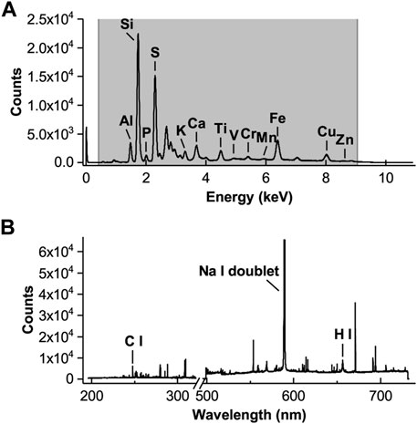
FIGURE 2. Typical measurement result of the LIBS-XRF instrument. (A) XRF spectrum. Data from gray area is used in model establishment. (B) LIBS spectrum. The spectral lines used for model establishment are marked.

According to the approach discussed in Section 2.3.1, the PLS models were established for the determination of calorific value, ash, volatile, and sulfur, respectively. For the calorific value, the model achieved 0.97 in R² and an RMSE of 0.46 MJ/kg. For ash, the model achieved 0.97 in R² and an RMSE of 1.00%. For volatile, the model achieved 0.77 in R² and an RMSE of 0.45%. For sulfur, the model achieved 0.94 in R² and an RMSE of 0.13%. For the samples of the performance test, RMSEPs for calorific value, ash, volatile, and sulfur were 0.68 MJ/kg, 1.62%, 0.32%, and 0.24%, respectively. The results are indicated in Table 1, and all data points for the model establishment and performance test are shown in Figure 6. As shown by these results, although cross-validation was performed in the model establishment for optimization, the model was still not adequate for unknown samples.

TABLE 1

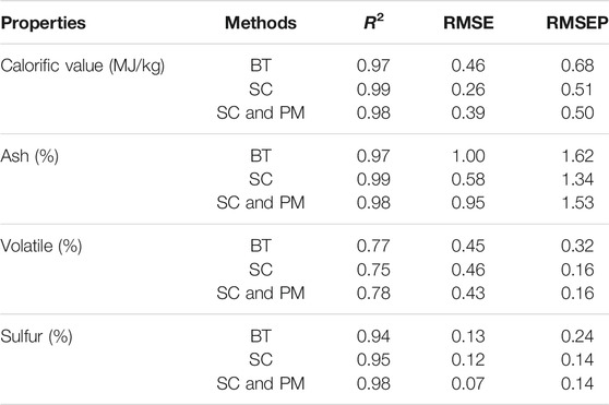
TABLE 1. The performance of the models based on basic data treatment, spectral intensity, correction, and piecewise modeling. BT, SC, and PM represent basic data treatment, spectral intensity correction, and piecewise modeling for short.

3.2 Spectral Intensity Correction

Figure 3 shows the signal fluctuations of the 15 XRF measurements of the standard sample during the measurements in the power plant. The relative standard deviations (RSDs) of several peak areas that are marked by numbers in Figure 3 are the error bars that are marked according to the RSDs. As shown in Figure 3, the intensity fluctuation was significant for channels of low energy, especially for the two high peaks, but for the higher channels, this phenomenon was barely observed. An RSD value below 0.01 can be treated as a normal fluctuation in the continuous measurements. Besides, the intentional changes of a little higher or lower vacuum in the measurements could not recurrent it, as we thought the phenomenon was perhaps caused by the attenuation of low-energy X-ray in air. Since the cause of the spectral intensity fluctuation was unclear, these results were used for the spectral intensity correction of following measurements after repeating the measurement of the standard sample. Therefore, new calibration models were established according to Section 2.3.2. For calorific value, the model achieved 0.99 in R² and an RMSE of 0.26 MJ/kg. For ash, the model achieved 0.99 in R² and an RMSE of 0.58%. For volatile, the model achieved 0.75 in R² and an RMSE of 0.46%. For sulfur, the model achieved 0.95 in R² and an RMSE of 0.12%. For the samples of the performance test, the RMSEPs for calorific value, ash, volatile, and sulfur were 0.51 MJ/kg, 1.34%, 0.16%, and 0.14%, respectively. These results are also indicated in Table 1, and all data points are also shown in Figure 6 for comparison. The results showed that the accuracy of calorific value, ash, and sulfur prediction was improved. Meanwhile, the models for the prediction of calorific value, ash, and sulfur themselves were better than before. But at the same time, the model for volatile prediction was not improved. This may be related to the elemental information–based model formation, which may have not been enough for volatile prediction. In addition, the R² for the volatile model was poor compared with other models.

FIGURE 3

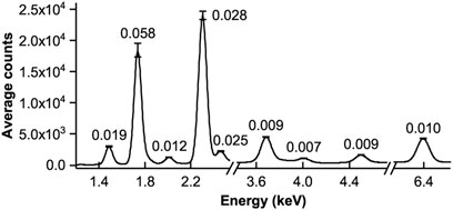
FIGURE 3. Spectral intensity fluctuation: a statistical expression of the 15 XRF measurements of the standard sample. The RSDs of the peak areas are marked by numbers. The error bars show the fluctuation according to the RSDs.

3.3 Piecewise Modeling

For the XRF signals after spectral intensity correction, the two lines around the S peak from channels 805 to 946 tend to group themselves by a clear boundary (Figure 4). Therefore, the PCA algorithm was first applied to the XRF signal from channels 805 to 946 after spectral intensity correction. The first principal components of the 316 samples for model establishment are shown in Figure 5. The first principal component explains 99.89% of the variance of the data. The samples are separated into two groups by their first principal components. The separation criteria were set at the middle of the separation (dash line in Figure 5).

FIGURE 4

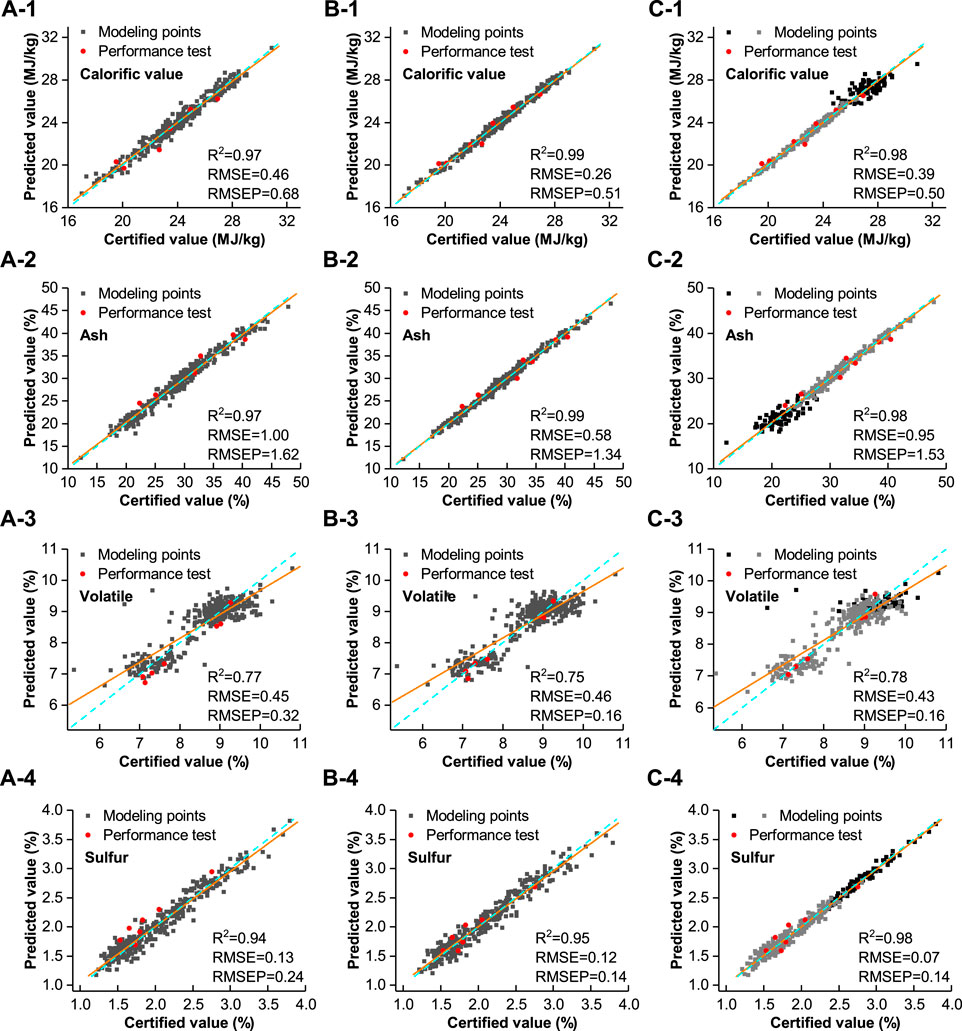
FIGURE 4. XRF channels 805–946 of the 316 modeling samples after spectral intensity correction. There is a clear gap between these two lines.

FIGURE 5

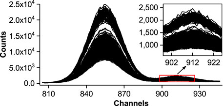
FIGURE 5. The first principal components of the 316 samples for model establishment. The separation criteria is shown by the dash line.

The piecewise modeling results are also indicated in Table 1, and all data points are also shown in Figure 6 for comparison. For calorific value, the model achieved 0.98 in R² and an RMSE of 0.39 MJ/kg. For ash, the model achieved 0.98 in R² and an RMSE of 0.95%. For volatile, the model achieved 0.78 in R² and an RMSE of 0.43%. For sulfur, the model achieved 0.98 in R² and an RMSE of 0.07%. For the samples of the performance test, the RMSEPs for calorific value, ash, volatile, and sulfur were 0.50 MJ/kg, 1.53%, 0.16%, and 0.14%, respectively. As the PCA results showed, the first principal component (PC1) dominated the differences between these signals, which means in fact the piecewise models were separated by the intensity of S signals. As a consequence, the model looks pretty better for sulfur prediction than the other methods, despite the similar result of prediction test as doing spectral intensity correction only. And for the volatile prediction, which has a strong relation to the sulfur content, the models and prediction performance seemed improved as well. The points for the performance test of volatile prediction were the closest to the line of y = x in the comparison between the different methods. On the other hand, the S-based piecewise criteria were not suitable for calorific value and ash prediction. As shown in Figure 6, better models for calorific value and ash were not achieved. The worse model performance for one of the sub-models may affect the accuracy of the whole model. For the other sub-models, the R²s and RMSEs were 0.99 and 0.18 MJ/kg for calorific value, and 0.98 and 0.59% for ash, which were at least as good as the spectral intensity correction models. Comparing the data sets of the two sub-models in Figure 6, this may be related to a lack of dynamic range in the model establishment in one of the sub-models.

FIGURE 6

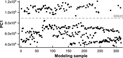
FIGURE 6. Comparison of the modeling results and performance test results. (A) Basic data treatment PLS model; (B) Spectral intensity correction PLS model; (C) Piecewise PLS model with spectral intensity correction. The marks 1–4 represent the results for calorific value, ash, volatile, and sulfur, respectively. The different types of modeling points are used to distinct the two sub-models in the piecewise models. The solid lines are linear fittings of modeling points and the dash lines are y = x lines.

4 Conclusion

In this work, the measurement results of the LIBS-XRF instrument were reassessed because of the long-term intensity fluctuation of the elemental lines in XRF signals. The spectral intensity correction method was introduced for improving the accuracy of the calibration models as well as for the prediction of unknown samples. Besides, the piecewise modeling was performed to make use of the characteristics observed in the signals. The modeling results were evaluated by their RMSEs, R²s, and RMSEPs of unknown samples. The performance of the models was improved after spectral intensity correction. The accuracy of the models on unknown samples was enhanced. For volatile and sulfur prediction of unknown samples, the piecewise modeling further enhanced the performance of the models. Therefore, the spectral intensity correction was recommended for calorific value and ash predictions, while together with piecewise modeling, the predictions for volatile and sulfur were recommended. Besides, as the results showed, the models for volatile prediction were poor in R²s, which was still a hidden trouble of unreliable predictions for unknown samples. On the other hand, the three-only data points from the LIBS signals wasted a lot of LIBS signals for stable elemental and non-elemental information, with which the model performance may be enhanced, which should be studied in the future.

Data Availability Statement

The raw data supporting the conclusion of this article will be made available by the authors, without undue reservation.

Author Contributions

YB, LZ, JL, WY, and SJ planned and supervised the experiments, and YB and LZ wrote and revised the manuscript. YB, JL, WZ, JH, YZ, FC, SW, GW, XM, ZL, and XL worked on data processing. All authors contributed to the article and approved the submitted version.

Funding

This work was financially supported by the National Key R&D Program of China (No. 2017YFA0304203); Changjiang Scholars and Innovative Research Team in the University of Ministry of Education of China (IRT_17R70); National Natural Science Foundation of China (NSFC) (Nos. 6197503, 61875108, 61775125, and 11434007); National Energy R&D Center of Petroleum Refining Technology (RIPP, SINOPEC); Major Special Science and Technology Projects in Shanxi (No. 201804D131036); 111 project (D18001); Fund for Shanxi “1331KSC”.

Conflict of Interest

Authors WZ, GW, XM, ZL, and XL were employed by Shanxi Xinhua Chemical Defense Equipment Research Institute Co. Ltd. Author SW was employed by the Research Institute of Petroleum Processing, SINOPEC.

The remaining authors declare that the research was conducted in the absence of any commercial or financial relationships that could be construed as a potential conflict of interest.

The authors declare that this study received funding from RIPP, SINOPEC. The funder had the following involvement in the study: providing the test site of the instrument.

Publisher’s Note

All claims expressed in this article are solely those of the authors and do not necessarily represent those of their affiliated organizations, or those of the publisher, the editors, and the reviewers. Any product that may be evaluated in this article, or claim that may be made by its manufacturer, is not guaranteed or endorsed by the publisher.

References

1. Maurice S, Wiens RC, Bernardi P, Cais P, Robinson S, Nelson T. The Supercam Instrument Suite on the mars 2020 Rover: Science Objectives and Mast-Unit Description. SPACE SCIENCE REVIEWS (2021) 217. doi:10.1007/s11214-021-00807-w

CrossRef Full Text | Google Scholar

2. Kwak J-h., Lenth C, Salb C, Ko E-J, Kim K-W, Park K Quantitative Analysis of Arsenic in Mine Tailing Soils Using Double Pulse-Laser Induced Breakdown Spectroscopy. Spectrochimica Acta B: At Spectrosc (2009) 64:1105–10. doi:10.1016/j.sab.2009.07.008

CrossRef Full Text | Google Scholar

3. Sheta S, Afgan MS, Hou Z, Yao S-C, Zhang L, Li Z. Coal Analysis by Laser-Induced Breakdown Spectroscopy: a Tutorial Review. J Anal Spectrom (2019) 34:1047–82. doi:10.1039/C9JA00016J

CrossRef Full Text | Google Scholar

4. Chu Y, Chen T, Chen F, Tang Y, Tang S, Jin H. Discrimination of Nasopharyngeal Carcinoma Serum Using Laser-Induced Breakdown Spectroscopy Combined with an Extreme Learning Machine and Random forest Method. J Anal Spectrom (2018) 33:2083–8. doi:10.1039/C8JA00263K

CrossRef Full Text | Google Scholar

5. Sun L, Yu H, Cong Z, Lu H, Cao B, Zeng P. Applications of Laser-Induced Breakdown Spectroscopy in the Aluminum Electrolysis Industry. Spectrochim Acta B (2018) 142:29–36. doi:10.1016/j.sab.2018.02.005

CrossRef Full Text | Google Scholar

6. Guo J, Lu Y, Cheng K, Song J, Ye W, Li N. Development of a Compact Underwater Laser-Induced Breakdown Spectroscopy (Libs) System and Preliminary Results in Sea Trials. Appl Opt (2017) 56:8196–200. doi:10.1364/ao.56.008196

PubMed Abstract | CrossRef Full Text | Google Scholar

7. Cai L, Wang Z, Li C, Huang X, Zhao D, Ding H. Development of an In Situ Diagnostic System for Mapping the Deposition Distribution on Plasma Facing Components of the Hl-2m Tokamak. Rev Sci Instrum (2019) 90:053503. doi:10.1063/1.5082630

PubMed Abstract | CrossRef Full Text | Google Scholar

8. Nicolodelli G, Senesi GS, Ranulfi AC, Marangoni BS, Watanabe A, de Melo Benites V. Double-pulse Laser Induced Breakdown Spectroscopy in Orthogonal Beam Geometry to Enhance Line Emission Intensity from Agricultural Samples. Microchemical J (2017) 133:272–8. doi:10.1016/j.microc.2017.03.047

CrossRef Full Text | Google Scholar

9. Zhang L, Dong L, Dou H, Yin W, Jia S. Laser-induced Breakdown Spectroscopy for Determination of the Organic Oxygen Content in Anthracite Coal under Atmospheric Conditions. Appl Spectrosc (2008) 62:458–63. doi:10.1366/000370208784046786

PubMed Abstract | CrossRef Full Text | Google Scholar

10. Yin W, Zhang L, Dong L, Ma W, Jia S. Design of a Laser-Induced Breakdown Spectroscopy System for On-Line Quality Analysis of Pulverized Coal in Power Plants. Appl Spectrosc (2009) 63:865–72. doi:10.1366/000370209788964458

PubMed Abstract | CrossRef Full Text | Google Scholar

11. Chen M, Yuan T, Hou Z, Wang Z, Wang Y. Effects of Moisture Content on Coal Analysis Using Laser-Induced Breakdown Spectroscopy. Spectrochim Acta B (2015) 112:23–33. doi:10.1016/j.sab.2015.08.003

CrossRef Full Text | Google Scholar

12. Yu Z, Yao S, Jiang Y, Chen W, Xu S, Qin H. Comparison of the Matrix Effect in Laser Induced Breakdown Spectroscopy Analysis of Coal Particle Flow and Coal Pellets. J Anal Spectrom (2021) 36:2473–9. doi:10.1039/d1ja00223f

CrossRef Full Text | Google Scholar

13. Feng J, Wang Z, Li L, Li Z, Ni W. A Nonlinearized Multivariate Dominant Factor–Based Partial Least Squares (Pls) Model for Coal Analysis by Using Laser-Induced Breakdown Spectroscopy. Appl Spectrosc (2013) 67:291–300. doi:10.1366/11-06393

PubMed Abstract | CrossRef Full Text | Google Scholar

14. Li X, Wang Z, Fu Y, Li Z, Ni W. A Model Combining Spectrum Standardization and Dominant Factor Based Partial Least Square Method for Carbon Analysis in Coal Using Laser-Induced Breakdown Spectroscopy. Spectrochim Acta B (2014) 99:82–6. doi:10.1016/j.sab.2014.06.017

CrossRef Full Text | Google Scholar

15. Hou Z, Wang Z, Yuan T, Liu J, Li Z, Ni W. A Hybrid Quantification Model and its Application for Coal Analysis Using Laser Induced Breakdown Spectroscopy. J Anal Spectrom (2016) 31:722–36. doi:10.1039/C5JA00475F

CrossRef Full Text | Google Scholar

16. Zhang Y, Xiong Z, Ma Y, Zhu C, Zhou R, Li X. Quantitative Analysis of Coal Quality by Laser-Induced Breakdown Spectroscopy Assisted with Different Chemometric Methods. Anal Methods (2020) 12:3530–6. doi:10.1039/d0ay00905a

PubMed Abstract | CrossRef Full Text | Google Scholar

17. Li XL, An SQ, Liu YX, Yu ZS, Zhang Q. Investigation of a High-Pressure Pressed Powder Pellet Technique for the Analysis of Coal by Wavelength Dispersive X-ray Fluorescence Spectroscopy. Appl Radiat Isotopes (2018) 132:170–7. doi:10.1016/j.apradiso.2017.11.003

CrossRef Full Text | Google Scholar

18. Wawrzonek L, Parus JL. Application of Multivariate Linear Regression for Determination of Ash Content in Coal by Xrf Analysis. Isotopenpraxis Isotopes Environ Health Stud (1988) 24:82–4. doi:10.1080/10256018808623904

CrossRef Full Text | Google Scholar

19. Ma K. Experimental Study on Determination of Major Elements in Coal Ash by X-ray Fluorescence Spectrometry. Coal Qual Technology (2019) 2, 32–5.

Google Scholar

20. Li X, Zhang L, Tian Z, Bai Y, Wang S, Han J. Ultra-repeatability Measurement of the Coal Calorific Value by Xrf Assisted Libs. J Anal Spectrom (2020) 35:2928–34. doi:10.1039/D0JA00362J

CrossRef Full Text | Google Scholar

21. Patro SK, sahu KK. Normalization: A Preprocessing Stage. IARJSET (2015) 2, 20–2. doi:10.17148/IARJSET.2015.2305

CrossRef Full Text | Google Scholar