Noise-Induced Aggregation of Swimmers in the Kolmogorov Flow

We investigate a model for the dynamics of ellipsoidal microswimmers in an externally imposed, laminar Kolmogorov flow. Through a phase-space analysis of the dynamics without noise, we find that swimmers favor either cross-stream or rotational drift, depending on their swimming speed and aspect ratio. When including noise, i.e., rotational diffusion, we find that swimmers are driven into certain parts of phase space, leading to a nonuniform steady-state distribution. This distribution exhibits a transition from swimmer aggregation in low-shear regions of the flow to aggregation in high-shear regions as the swimmer’s speed, aspect ratio, and rotational diffusivity are varied. To explain the nonuniform phase-space distribution of swimmers, we apply a weak-noise averaging principle that produces a reduced description of the stochastic swimmer dynamics. Using this technique, we find that certain swimmer trajectories are more favorable than others in the presence of weak rotational diffusion. By combining this information with the phase-space speed of swimmers along each trajectory, we predict the regions of phase space where swimmers tend to accumulate. The results of the averaging technique are in good agreement with direct calculations of the steady-state distributions of swimmers. In particular, our analysis explains the transition from low-shear to high-shear aggregation.

1 Introduction

The interaction between self-propelled particles and fluid flows is central to many active matter systems, including swimming bacteria [1], Janus particles [2, 3], and microtubule-based active nematics [4]. A key issue for these systems is understanding how the combined effects of fluid advection and self-propulsion determine the macroscopic properties of the active suspension. This is a nontrivial question even for dilute suspensions of active particles subjected to externally imposed, time-independent fluid flows. In this case, connecting the behavior of individual particles to the macroscopic properties of the fluid-particle suspension may be difficult because active particles can exhibit chaotic dynamics in such flows, e.g., vortex flows [5–9].

For sufficiently simple flows—such as time-independent planar shear flows—swimmers do not exhibit chaos, but the connection between the swimmer trajectories and the macroscopic properties of the suspension has remained elusive. Experiments on swimming microorganisms in microfluidic channel flows reveal that the swimmer concentration profile is nonuniform across the channel and dependent on the type of microorganism and the ratio of the swimming speed relative to the flow speed [1, 10]. Intriguingly, for certain species, the shape of the concentration profile exhibits a transition from being peaked on either side of the channel center to being peaked at the center of the channel as the flow speed increases [10]. Because the magnitude of the fluid shear is peaked at the edges of the channel and goes to zero at the center of the channel, this is characterized as a transition from low-shear depletion to high-shear depletion. In Ref. [1], it is shown that in order to capture this key feature of the experimental data, the model for swimmer motion must take into account fluctuations in the swimming direction caused by rotational diffusion or run-and-tumble swimming. In particular, a Fokker-Planck model [11] predicts a transition from low-shear to high-shear depletion in channel flows as a function of swimmer shape and rotational diffusivity, consistent with the experiments [10].

The Fokker-Planck model provides an accurate quantitative description of the swimmer density in the channel flow, but it does not provide a clear mechanism for the transition from low-shear to high-shear depletion. In particular, it obscures the link between the concentration profile and the swimmer trajectories one actually observes in the presence of both fluid flows and rotational noise. It also leaves open the question of how nonuniform distributions in the swimmer’s phase space arise in the first place, given that typical models of swimmer motion in planar shear flows are conservative dynamical systems perturbed by noise [12–14]. Because conservative systems cannot possess attractors, which typically account for the high-density regions of phase space in noisy dynamical systems, the cause of density variations in the swimmer phase space is more subtle. For elongated swimmers in planar shear flows, the dynamics is conservative but non-Hamiltonian, similar to the case of elongated swimmers in axisymmetric vortex flows [15]. Therefore, the dynamics does not locally preserve phase-space volume, and consequently density variations occur even in the absence of noise. When noise is included, however, the swimmer distributions clearly favor certain trajectories over others, an effect that cannot be accounted for by the non-Hamiltonian character of the dynamics.

In this paper, we study a model of an elongated swimmer in a planar Kolmogorov flow and elucidate the connection between the swimmer trajectories with noise and the swimmer density in phase space. We choose to study the planar Kolmogorov flow—that is, a spatially periodic, alternating shear flow—rather than the channel flow, because this allows us to ignore the effect of boundary conditions on the swimmer dynamics, which can be quite complex and system dependent [16]. We calculate the steady-state distributions of swimmers in the flow numerically, which exhibit nonuniform concentration profiles in the cross-stream direction that are similar to those observed in channel flows. In particular, we map out the transition from low-to high-shear depletion as a function of swimmer speed, shape, and rotational diffusivity. Then, taking advantage of a conserved quantity possessed by our model, we derive a reduced drift-diffusion model for the swimmer dynamics in the limit of weak noise. The reduced model allows us to calculate the likelihood of observing particular swimmer trajectories in the presence of noise. Combining this with the slow-down of trajectories in phase-space, we are able to fully explain the nonuniformity of the swimmer steady-state distributions. The predictions of the reduced model are quantitatively accurate in the small-diffusion limit and explain the transition from low-to high-shear depletion in terms of the relative weighting of different swimmer trajectories.

This paper is organized as follows. In Sec. 2, we describe the phase-space structure of the swimmer in the Kolmogorov flow without noise. In Sec. 3, we add rotational diffusion to our model and calculate the probability density and depletion of swimmers in the Kolmogorov flow as a function of swimmer speed, shape, and rotational diffusivity. In Sec. 4, we introduce the reduced model for swimmer dynamics with weak diffusion, and we use the model to explain our observations from the previous section. Concluding remarks are in Sec. 5. Supplementary Appendix A1 contains details of our numerical method for solving the swimmer Fokker-Planck equation.

2 Deterministic Dynamics of a Swimmer in the Kolmogorov Flow

The 2D, laminar Kolmogorov flow is given by

$\mathbf{\text{u}}=\left(U\cos \left(\frac{y}{w}\right),0\right).(1)$

Here the constant U is the maximum fluid speed at y = 0 and y = ±πw, where 2πw is the spatial period of the flow. We refer to y = 0 and y = ±πw as the centerlines of the flow, in analogy with the Poiseuille flow, which has maximum speed on the centerline of the channel. In the Kolmogorov flow, the equations of motion of an ellipsoidal swimmer with position r = (x, y) and swimming direction θ relative to the x axis, as shown in Figure 1, are [5, 9].

$\dot{x}=u_x+V\cos \theta =U\cos \left(\frac{y}{w}\right)+V\cos \theta ,(\mathrm{2a})$

$\dot{y}=u_y+V\sin \theta =V\sin \theta ,(\mathrm{2b})$

$\dot{\theta }=\frac{1}{2}\left(u_{y,x}-u_{x,y}\right)+\alpha \left[\frac{1}{2}\left(u_{x,y}+u_{y,x}\right)\cos 2\theta -u_{x,x}\sin 2\theta \right]=\frac{U}{2w}\sin \left(\frac{y}{w}\right)\left[1-\alpha \cos 2\theta \right],(\mathrm{2c})$

where the first equality in Eq. 2c is Jeffery’s equation for an ellipsoidal particle in an incompressible flow [17]. We have used the notation (⋅)_,x ≡ ∂(⋅)/∂x. The parameter V is the swimming speed, and α = (γ² − 1)/(γ² + 1) is the swimmer shape parameter, where γ is the ellipsoid aspect ratio. The parameter α takes values between −1 and 1, with α = 1 corresponding to a rod swimming parallel to its major axis, α = 0 corresponding to a circular swimmer, and α = −1 corresponding to a rod swimming perpendicular to its major axis. A schematic of the model is shown in Figure 1.

FIGURE 1

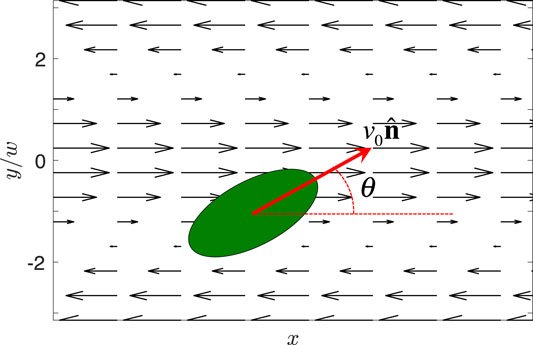
FIGURE 1. Schematic of an ellipsoidal swimmer with shape parameter 0 < α < 1 in the Kolmogorov flow (not to scale).

In this paper, we focus on the dynamics in the (y, θ) plane, since the system is translationally invariant in the x direction. Furthermore, we work with the non-dimensionalized version of Eq. 1, which we obtain by normalizing by the velocity scale U and the length scale w. This leads to

$\dot{y}=v_0\sin \theta ,(\mathrm{3a})$

$\dot{\theta }=\frac{\sin y}{2}\left[1-\alpha \cos 2\theta \right],(\mathrm{3b})$

with the rescaled swimming speed v₀ = V/U. Because Eq. 3 is periodic in both y and θ, we interpret the phase space topologically as a two torus, i.e., a donut. Remarkably, system (3) is conservative, as is the dynamics of ellipsoidal swimmers in 2D and 3D Poiseuille flows [12, 13], spherical gyrotactic swimmers in Kolmogorov flows [14], and spherical swimmers in 2D vortex flows [15]. The conserved quantity may be derived in the standard way. Dividing Eq. 3a by Eq. 3b, we obtain

$\frac{\mathrm{d}y}{\mathrm{d}\theta }=\frac{2v_0\sin \theta }{\sin y\left(1-\alpha \cos 2\theta \right)}.(4)$

Separating variables in Eq. 4, we obtain

$\sin y\mathrm{d}y=\frac{2v_0\sin \theta }{1-\alpha \cos 2\theta }\mathrm{d}\theta .(5)$

Eq. 5 may be integrated, which introduces an integration constant Ψ. This implies that Ψ (y, θ) is a constant of motion, and it is given by

$\mathrm{\Psi }\left(y,\theta \right)=\left\{\begin{array}{cc}\cos y-2v_0\frac{{\tanh }^{-1}\left(\sqrt{\frac{2\alpha }{1+\alpha }}\cos \theta \right)}{\sqrt{2\alpha \left(1+\alpha \right)}},\hfill & \mathrm{f}\mathrm{o}\mathrm{r}0<\alpha \le 1,\hfill \\ \cos y-2v_0\cos \theta ,\hfill & \mathrm{f}\mathrm{o}\mathrm{r}\alpha =0,\hfill \\ \cos y-2v_0\frac{{\tan }^{-1}\left(\sqrt{\frac{2|\alpha |}{1+\alpha }}\cos \theta \right)}{\sqrt{2|\alpha |\left(1+\alpha \right)}},\hfill & \mathrm{f}\mathrm{o}\mathrm{r}-1<\alpha <0.\hfill \end{array}\right.(6)$

When α = 0, i.e., for circular swimmers, Eq. 3 has a Hamiltonian structure $\dot{y}=\partial H/\partial \theta$, $\dot{\theta }=-\partial H/\partial y$, with the Hamiltonian H (y, θ) = Ψ (y, θ)/2. This implies that the phase-space area dydθ is preserved by the dynamics. On the other hand, for elongated swimmers (α ≠ 0), Eq. 3 is non-Hamiltonian, similar to swimmers in Poiseuille flows [13] and axisymmetric vortex flows [15]. Hence, phase-space area is not preserved in this case.

As a result, each trajectory of Eq. 3 lies on a constant-Ψ contour and the phase space is foliated by periodic trajectories almost everywhere. Illustrative phase portraits are shown in Figures 2A–C for α = 0.9 and Figures 2D–F for α = −0.7. The phase portraits are organized around the four fixed points of Eq. 3. For all v₀ and all α < 1, the fixed points are (y₁, θ₁) = (0, 0), (y₂, θ₂) = (0, π), (y₃, θ₃) = (π, π) and (y₄, θ₄) = (π, 0). The fixed points (y₁, θ₁) and (y₃, θ₃) are saddles, while (y₂, θ₂) and (y₄, θ₄) are centers, and the two fixed points within each pair map into each other by the shift-flip symmetry

$\left(y,\theta \right)\mapsto \left(y+\pi ,\pi -\theta \right)(7)$

FIGURE 2

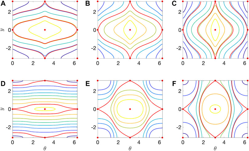
FIGURE 2. Phase portraits of Eq. 3 for (A–C) α = 0.9 and (D–F) α = − 0.7. (A) v₀ = 0.2. (B) v₀ = v*(α) = 0.430. (C) v₀ = 0.8. (D) v₀ = 0.02. (E) v₀ = v*(α) = 0.285. (F) v₀ = 0.6. Red dots are the fixed points of Eq. 3. Red curves are the separatrices emanating out of the saddle fixed points at (y, θ) = (0, 0) and (y, θ) = (±π, π). The color of each remaining curve corresponds to a distinct value of Ψ.

of Eq. 3. The centers are surrounded by periodic orbits, as shown in Figure 2. This can either be viewed as a consequence of the conservative nature of the system, or a consequence of the time-reversal symmetries

$\left(y,\theta ,t\right)\mapsto \left(y,-\theta ,-t\right),(\mathrm{8a})$

$\left(y,\theta ,t\right)\mapsto \left(-y,\theta ,-t\right).(\mathrm{8b})$

Indeed, all of the fixed points are invariant under both of the symmetries (8), in particular the centers, which guarantees that they are surrounded by periodic orbits [18].

The time-reversal symmetries (8) also force the invariant manifolds of the saddles to be homoclinic orbits. These homoclinic orbits (red curves in Figure 2) act as separatrices between two topologically distinct types of periodic trajectories (Figures 2A,C,D,F). Either 1) a trajectory is enclosed by the separatrices of a saddle, and hence wraps around the center inside the separatrices, or 2) the trajectory is in between the separatrices of the two saddles, and hence does not wrap around a center. In other words, the homoclinc orbits separate orbits which are 1) contractible on the torus from those which are 2) non-contractible. We refer to the regions enclosed by a saddle’s separatrices as the islands, and the remaining regions as jets.

For sufficiently small v₀ (Figures 2A,D), the spatially varying shear suppresses sustained cross-stream drift and promotes rotational drift. The islands contain swimmer trajectories that oscillate around the centerlines, while the swimmer’s orientation oscillates back and forth, never completing a 2π rotation. Meanwhile, the jets contain swimmer trajectories that oscillate in the y direction, never crossing the centerlines, while the swimmer orientation continuously drifts either clockwise or counterclockwise. On the other hand, for sufficiently large v₀, (Figures 2C,F), a swimmer’s self-propulsion can prevail and give rise to sustained motion in the y-direction. While the islands are qualitatively similar to the small v₀ case, the jets now either transport swimmers in the +y or −y direction, depending on θ. In these jets, a swimmer’s orientation never completes a full rotation, but oscillates around θ = π/2 or θ = 3π/2, respectively.

The transition from rotational drift to cross-stream drift in the jets occurs at a shape-dependent swimming speed v^∗(α), at which system (3) exhibits a global bifurcation. The bifurcation takes place when the separatrices of each of the saddle points coincide exactly, as shown in Figures 2B,E. This occurs when the level sets containing the saddles (0, 0) and (π, π) are identical, meaning Ψ (0, 0) = Ψ (π, π). Using Eq. 6, this relation leads to v^∗(α), given by

$v^{\ast }\left(\alpha \right)=\left\{\begin{array}{cc}\frac{\sqrt{2\alpha \left(1+\alpha \right)}}{2{\tanh }^{-1}\left(\sqrt{\frac{2\alpha }{1+\alpha }}\right)},\hfill & \text{for\hspace{0.17em}}0<\alpha <1,\hfill \\ \frac{1}{2},\hfill & \text{for\hspace{0.17em}}\alpha =0,\hfill \\ \frac{\sqrt{2|\alpha |\left(1+\alpha \right)}}{2{\tan }^{-1}\left(\sqrt{\frac{2|\alpha |}{1+\alpha }}\right)},\hfill & \text{for\hspace{0.17em}}-1\le \alpha <0.\hfill \end{array}\right.(9)$

The bifurcation curve is plotted in Figure 3. This transition from rotational to cross-stream drift is an interesting aspect of the swimmer dynamics in the Kolmogorov flow, which has no direct counterpart in channel flows. A similar phenomenon has been observed numerically for gyrotactic swimmers in the Kolmogorov flow [14].

FIGURE 3

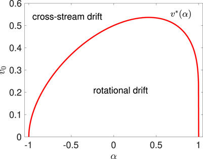
FIGURE 3. Swimmer phase space structure as a function of the swimming speed v₀ and shape parameter α, where α = 0 corresponds to circular particles. The red curve is v*(α) (Eq. 9), the set of parameters where the saddles are heteroclinically connected and phase space bifurcates from containing rotational drift trajectories to cross-stream drift trajectories.

3 Stochastic Dynamics and Noise-Driven Aggregation

In both laboratory experiments and nature, real swimmers are subject to fluctuations in their motion which cause their trajectories to deviate from Eq. 3. We consider the situation where the swimming direction Eq. 3b is perturbed by white noise, while the translational motion continues to follow Eq. 3a. This description is a simple model for biological microswimmers, like swimming bacteria. For such swimmers, translational fluctuations are negligible compared to their self-propulsion, but rotational fluctuations are significant due to the fluctuating active forces that propel the swimmer [19, 20] and potentially run-and-tumble behavior as well [1]. Eq. 3 is replaced by the stochastic differential equation

$\mathrm{d}y=v_0\sin \theta \mathrm{d}t,(\mathrm{10a})$

$\mathrm{d}\theta =\frac{\sin y}{2}\left[1-\alpha \cos 2\theta \right]\mathrm{d}t+\sigma \mathrm{d}W,(\mathrm{10b})$

where σ is the dimensionless strength of rotational diffusion. In Eq. 10b, dW is the infinitesimal increment of a Wiener process, meaning for every instant of time t, dW is a zero-mean normally-distributed random variable with variance dt. We denote a particular realization of the Wiener process as $W(t)={\int }_0^t\mathrm{d}W$. The noise strength σ can be expressed in terms of the rotational diffusivity D_R as

$\sigma =\sqrt{\frac{2D_{R}w}{U}}=\sqrt{\frac{2}{{\mathrm{P}\mathrm{e}}_R}},(11)$

where Pe_R = U/D_Rw is the rotational Péclet number.

3.1 Steady-State Probability Density

Of particular interest is the steady-state probability density P (y, θ) of Eq. 10, which has been measured in experiments on the channel flow [1, 10]. The density P satisfies the steady-state Fokker-Planck equation associated with Eq. 10 [21, 22],

$-v_0\sin \theta \frac{\partial P}{\partial y}-\frac{\sin y}{2}\frac{\partial }{\partial \theta }\left[\left(1-\alpha \cos 2\theta \right)P\right]+\frac{{\sigma }^2}{2}\frac{{\partial }^{2}P}{\partial {\theta }^2}=0.(12)$

For circular swimmers, α = 0 and Eq. 12 is linear in the partial derivatives of P. Hence, the uniform distribution P = const is a solution, and for σ ≠ 0, we suspect that this solution is unique. Therefore, perfectly circular swimmers with rotational diffusion attain a uniform distribution in phase space. This is to be expected, given that the dynamics in the absence of noise is Hamiltonian and thus area-preserving, and the added noise is isotropic. For α ≠ 0 on the other hand, we expect a non-uniform steady-state distribution, due in part to the non-Hamiltonian nature of the deterministic dynamics. The periodicity of Eq. 12 in y and θ means it is straightforward to solve numerically using Fourier transforms. This aspect also makes the Kolmogorov flow more convenient to work with than a channel flow. We describe our numerical method in Supplementary Appendix A1, and our code is available in Ref. [23]¹. Example solutions are plotted in Figure 4. The plots are centered on one of the stable equilibria, (y, θ) = (0, π), and the separatrices enclosing each island are shown as the dotted red curves. The density inside the central y ∈ [ −π/2, π/2] region corresponds to rightward fluid flow (in the x direction), and it is related to the density in the leftward-flow region by the symmetry (7). When α ≠ 0, Figure 4 shows that P (y, θ) is highly nonuniform, featuring sharp peaks in certain regions.

FIGURE 4

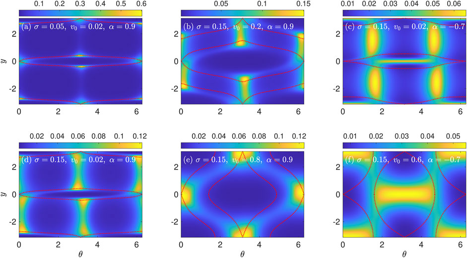
FIGURE 4. Steady-state probability densities P (y, θ) for various combinations of σ, v₀, and α indicated on each panel. Red dotted curves are the separatrices emanating from the saddles (y, θ) = (0, 0) and (y, θ) = (±π, π). Panels (A–D) are for parameters before the bifurcation from rotational to cross-stream drift, and panels (E) and (F) are after this bifurcation.

For α > 0 (i.e., swimming parallel to the particle’s long axis) and swimming speeds below the bifurcation [v₀ < v^∗(α), Figures 4A,B,D], the density is mostly concentrated near θ = 0 and π, with the y position of each peak lying close to the separatrices between the islands and the jets. At these angles, the deterministic part of the angular velocity [Eq. 10b] is minimized, meaning the swimmer spends more time near θ = 0 and π. Hence, this explains the increased density around those angles. When the noise is small (Figure 4A), there are three peaks around each island: one at the saddle point at θ = 0 (which appears as two peaks in Figure 4 due to our cutting the torus at θ = 0), and one on each side of the separatrix. Meanwhile, the density in the center of the islands, around the center equilibrium points, is small and at a local minimum. This suggests that the centers are unstable with respect to perturbations from rotational diffusion, which is not a priori obvious since centers are linearly stable. The small-noise distribution (Figure 4A) approximately respects the time-reversal symmetries (8). As rotational diffusion increases (Figure 4D), the peak around the saddle point splits into two peaks, and the distributions increasingly break the time-reversal symmetries. This is evidenced by the asymmetry of Figure 4D with respect to reflections about y = 0 and reflections about θ = π. The increased noise also causes the peaks near the saddle at (y, θ) = (0, 0) = (0, 2π) to begin merging with the peaks along the middle of the separatrix surrounding the island centered on y = ±π. This merging becomes more pronounced for higher v₀, because the separatrices get closer together (Figure 4B).

For α > 0 and swimming speeds above the bifurcation (Figure 4E), the density is peaked on both of the saddles, with most of the remaining density concentrated in the cross-stream jet region. The occurrence of peaks on the saddles may be surprising, because these fixed points are linearly unstable and hence one might not expect density to accumulate nearby. Again, the density inside the islands is small. Hence, we can sum up the behavior of α > 0 swimmers as follows. The effect of small noise is to eject swimmers from the centers of the islands and make them aggregate near the separatrices. Increasing the intensity of noise tends to preferentially push the swimmer density into the jet region, as seen when comparing Figures 4A,D, but the density is still strongly peaked at specific angles near θ = 0 and π. The aggregation of swimmer density near the separatrices is consistent with similar behavior seen in Monte Carlo simulations of swimmers in Poiseuille flow [1]. These effects are more pronounced the more elongated a swimmer is, i.e., the closer α is to 1. As α → 0 and the swimmer shape becomes more circular, the distribution P (y, θ) tends towards the uniform distribution, so the aggregation effects gradually diminish.

On the other hand, for α < 0 (i.e., swimming perpendicular to the particle’s long axis), the density is peaked both at the center fixed points and away from the islands at the angles θ = π/2 and 3π/2 (Figures 4C,F). When v₀ is small and below the bifurcation, the peaks around the centers have a narrow width in the y direction, as seen in Figure 4C. Meanwhile, there are prominent peaks for θ = π/2 and 3π/2 in the jet region. These angles correspond to the minimal angular speeds in Eq. 10b for the α < 0 case, where the swimmers spend more time. The peaks around the centers suggest that for α < 0, the centers are metastable with respect to perturbations from rotational diffusion. This is a stark difference from the α > 0 case, for which P (y, θ) is at a local minimum at the centers, and it is all the more striking because the linear stability type of the center fixed points does not depend on α. As v₀ increases, the peaks around the centers intensify while the peaks at θ = π/2 and 3π/2 gradually fade. For a sufficiently large v₀ (Figure 4F), the peaks at the centers completely dominate the probability distribution. Though we have selected a v₀ above the bifurcation in Figure 4F, the peaks at the centers become dominant compared to those at θ = π/2 and 3π/2 for values of v₀ well below the bifurcation. This behavior is revealed by examining the swimmer cross-stream concentration profiles.

3.2 Cross-Stream Concentration Profile and Depletion

Using the calculated densities P (y, θ), we investigate the depletion of swimmers from low- or high-shear regions of the flow, which is known to exhibit a complex dependence on the swimmer parameters (v₀, α, σ). Following prior work [1, 10, 11], we define a depletion index to quantify the nonuniformity of the spatial distribution of swimmers. The spatial distribution is given by

$C\left(y\right)={\int }_0^{2\pi }P\left(y,\theta \right)\mathrm{d}\theta .(13)$

The depletion index I_D is defined by computing the ratio of the concentration in the low-shear regions of the flow to the uniform concentration, and subtracting this from 1. For Poiseuille flows, the cutoff for the low-shear region is usually taken to be the central half-width of the channel. In the case of the Kolmogorov flow, which is like a periodically alternating Poiseuille flow, we take a similar definition as the central half-width of a region in which the flow points in one direction. Hence, we define I_D as

$I_D=1-2\left({\int }_{-\pi /4}^{\pi /4}C\left(y\right)\mathrm{d}y+{\int }_{3\pi /4}^{\pi }C\left(y\right)\mathrm{d}y+{\int }_{-\pi }^{-3\pi /4}C\left(y\right)\mathrm{d}y\right).(14)$

The first term in Eq. 14 is the concentration in the rightward low-shear region, and the second two terms comprise the concentration in the leftward low-shear region (see Figure 1). For a uniform density, I_D = 0; for low-shear depletion of swimmers, I_D > 0; for high-shear depletion, I_D < 0.

Example results of these calculations are shown in Figure 5 for the parameters used in Figure 4. We observe a diverse set of concentration profiles that reflect the strong dependence of the density P (y, θ) on the system parameters. For α > 0 and small v₀ (Figures 5A,D), C(y) is peaked on either side of each centerline as a result of the large peaks along the separatrices seen in Figures 4A,D. Because the islands are very narrow in the y direction when v₀ is small, the concentration peaks on either side of the centerline are close together. Hence, we obtain a negative depletion index, indicating high-shear depletion. For higher values of v₀, the separatrices [and the peaks of P (y, θ)] move away from the centerlines (Figure 4B), leading to a positive depletion index (Figure 5B). However, when v₀ is sufficiently large and past the bifurcation, the accumulation of density on the saddles at y = 0 and ±π (Figure 4E) leads again to a negative depletion index (Figure 5E). For α < 0 and small v₀ (Figure 5C), the concentration profile has peaks both at the centerlines and in the high-shear regions, owing to the P (y, θ) peaks at the centers and the jet regions, respectively (Figure 4C). Whether one observes a positive or negative I_D depends on the relative prominence of these two sets of peaks in phase space. As v₀ increases and the peaks at the centers dominate (Figure 4F), the swimmer concentration only features peaks at the centerlines (Figure 5F), leading to a negative depletion index.

FIGURE 5

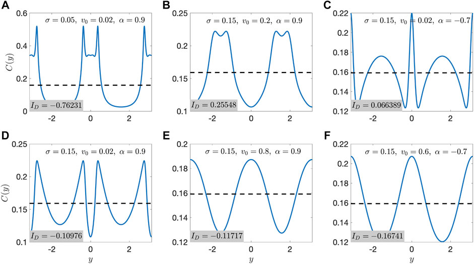
FIGURE 5. Concentration profiles C(y) for various combinations of σ, v₀, and α corresponding to those used in Figure 4. Panels A–D are for parameters before the bifurcation from rotational to cross-stream drift, and panels E and F are after this bifurcation. The dashed lines show the uniform concentration profile, to highlight the nonuniformity of the swimmer concentrations C(y). The depletion index I_D for each parameter is noted on each panel.

We perform a systematic exploration of the (v₀, α, σ) parameter space. The results are plotted in Figure 6 as isosurfaces of I_D. The transitions from high-shear to low-shear depletion (I_D < 0 to I_D > 0) are indicated by the grey surfaces. Clearly, these transitions are highly dependent on v₀ and α, though they only depend weakly on σ for the range of σ values considered here. Surprisingly, the transitions appear to be independent of the bifurcation in the swimmer phase space discussed in Sec. 2, indicated by the black dotted curve in Figure 6.

FIGURE 6

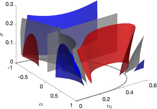
FIGURE 6. Isosurfaces of the depletion index I_D in the (v₀, α, σ) parameter space. Blue surfaces: I_D = −0.15. Grey surfaces: I_D = 0. Red surfaces: I_D = 0.1. The black dotted curve in the (v₀, α) plane is the bifurcation curve shown in Figure 3.

The speed- and shape-dependent depletion behavior of swimmers in the Kolmogorov flow is similar to the experimental observations reported in Refs. [1, 10] for a channel flow. These experiments measured C(y) and I_D as a function of maximum flow speed for several swimming microorganisms, with differing shapes and stroke patterns. We qualitatively mimic this type of experiment by taking cuts of Figure 6 at fixed σ and α, leading to I_D (v₀) as plotted in Figure 7. High v₀ corresponds to low flow speed, while small v₀ corresponds to high flow speed. Figure 7 shows that in all cases where α > 0, the depletion index is maximized at an intermediate v₀. Furthermore, for extremely elongated swimmers such that α is close to 1, I_D > 0 for a wide range of v₀ (Figure 7C). These observations are consistent with experiments on slender swimming bacteria in channel flows, which found that I_D > 0 and is maximized for an intermediate flow speed [1]. On the other hand, for more rounded swimmers for which α is closer to 0, the depletion index goes from positive to negative as v₀ decreases, staying negative over a fairly wide range of v₀ (Figures 7A,B). This is indicative of a transition from low-to high-shear depletion with increasing flow speed, which has been observed in experiments on motile phytoplankton in channel flows [10]. The most extreme high-shear depletion with increasing flow speed depends on σ and α. For the value of σ used in Figure 7, I_D (v₀) becomes most negative with decreasing v₀ for intermediate values of α (i.e., intermediate aspect ratios, Figure 7B), while the effect is much more modest when α is close to 0 (Figure 7A, aspect ratio close to 1).

FIGURE 7

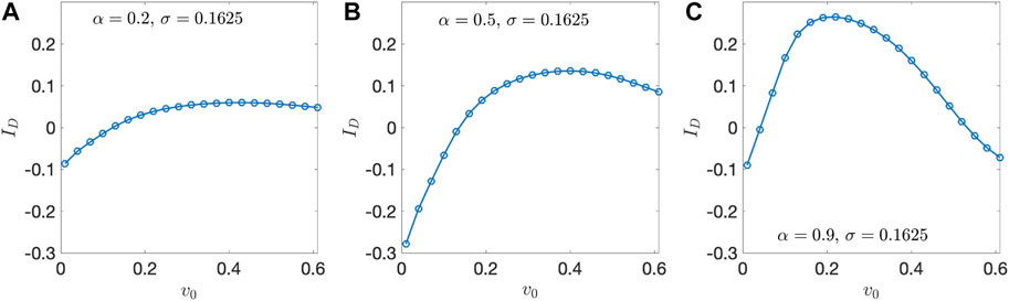
FIGURE 7. Depletion index I_D dependence on v₀ for selected values of α > 0 and σ = 0.1625. (A) α = 0.2. (B) α = 0.5. (C) α = 0.9.

4 Weak-Noise Behavior via the Averaging Principle

In Sec. 3, we showed that rotational diffusion leads to a pronounced, nonuniform probability density of swimmers in phase space. Nonuniform steady states are typical for dissipative—i.e., non-conservative—dynamical systems perturbed by noise. In that case, the probability density is peaked around the dissipative system’s attractors (e.g., stable fixed points or limit cycles) and is shaped by the balance between diffusion and phase space contraction around the attractors. In our case, Eq. 3 is conservative, meaning the phase space does not possess attractors. Hence, the dynamics of Eq. 3 alone cannot explain the regions of phase space where the swimmer density accumulates. This effect is specifically caused by the interplay between rotational diffusion and conservative dynamics in Eq. 10 [1]. In this section, we derive a model that captures this interplay by applying an averaging principle for conservative systems that is valid in the weak-noise limit. The result is a reduced drift-diffusion model that describes how a swimmer randomly moves across the deterministic orbits of its phase space. This model allows us to decompose the swimmer’s steady-state distribution P (y, θ) into the product of a probability density on the space of swimmer orbits, parametrized by the deterministic constant of motion Ψ, and a kinematic factor accounting for the orientation-dependent angular velocity of elongated particles.

4.1 Reduced Drift-Diffusion Model

To gain insight into the interplay between noise and the conservative dynamics, we calculate the evolution equation for the function Ψ (y(t), θ(t)) under Eq. 10. Because Ψ is a function of the stochastic process (y(t), θ(t)), its evolution equation must be derived using Itô’s Lemma [24], which yields the stochastic differential equation

$\mathrm{d}\mathrm{\Psi }=\frac{{\sigma }^2}{2}\frac{{\partial }^2\mathrm{\Psi }}{\partial {\theta }^2}\mathrm{d}t+\sigma \frac{\partial \mathrm{\Psi }}{\partial \theta }\mathrm{d}W.(15)$

When σ = 0, dΨ = 0, which implies the conservation of Ψ with no noise, as expected. Obviously, noise introduces dissipation, in the sense that Ψ is no longer conserved. When Eq. 15 is integrated, we obtain

$\mathrm{\Psi }\left(t\right)-\mathrm{\Psi }\left(0\right)=\frac{{\sigma }^2}{2}{\int }_0^t\frac{{\partial }^2\mathrm{\Psi }}{\partial {\theta }^2}\left(y\left(t^{\prime }\right),\theta \left(t^{\prime }\right)\right)\mathrm{d}{t}^{\prime }+\sigma {\int }_0^t\frac{\partial \mathrm{\Psi }}{\partial \theta }\left(y\left(t^{\prime }\right),\theta \left(t^{\prime }\right)\right)\mathrm{d}W.(16)$

Clearly, when σ is very small, Eq. 16 implies Ψ changes very slowly. We accordingly rescale time as t = τ/σ², under which dW↦σ⁻¹dW, so that Eq. 16 becomes

$\mathrm{\Psi }\left(\tau \right)-\mathrm{\Psi }\left(0\right)=\frac{1}{2}{\int }_0^{\tau }\frac{{\partial }^2\mathrm{\Psi }}{\partial {\theta }^2}\left(y\left({\tau }^{\prime }\right),\theta \left({\tau }^{\prime }\right)\right)\mathrm{d}{\tau }^{\prime }+{\int }_0^{\tau }\frac{\partial \mathrm{\Psi }}{\partial \theta }\left(y\left({\tau }^{\prime }\right),\theta \left({\tau }^{\prime }\right)\right)\mathrm{d}W.(17)$

For sufficiently small σ, a swimmer will complete many oscillations around a periodic orbit at a fixed Ψ (see Figure 2) before its Ψ value will have drifted appreciably. Hence, its motion may be decomposed into fast motion around the deterministic periodic orbits at fixed Ψ, and slow motion transverse to the periodic orbits, caused by noise. In the σ → 0 limit, we can thus approximate the terms on the right-hand side of Eq. 17 by averaging them over one period of the current orbit at fixed Ψ. This averaging principle is derived rigorously for general two-dimensional conservative dynamical systems perturbed by white noise in Ref. [25] and references therein. We describe the technique here and apply it to the swimmer in the Kolmogorov flow.

The averaged equations are as follows. The assumption that Ψ changes slowly implies that the integrand of the first term of Eq. 17 can be approximated by its average value over one period of the orbit with fixed Ψ, which we denote by f(Ψ). The function f is given by

$f\left(\mathrm{\Psi }\right)=\frac{1}{2T\left(\mathrm{\Psi }\right)}\oint \frac{{\partial }^2\mathrm{\Psi }}{\partial {\theta }^2}\mathrm{d}{\tau }^{\prime },(18)$

where T(Ψ) is the period of this orbit, and

$\frac{1}{2}{\int }_0^{\tau }\frac{{\partial }^2\mathrm{\Psi }}{\partial {\theta }^2}\left(y\left({\tau }^{\prime }\right),\theta \left({\tau }^{\prime }\right)\right)\mathrm{d}{\tau }^{\prime }\approx {\int }_0^{\tau }f\left(\mathrm{\Psi }\left({\tau }^{\prime }\right)\right)\mathrm{d}{\tau }^{\prime }.(19)$

Meanwhile, a standard result from stochastic processes, proved in Supplementary Appendix A2, is that the stochastic integral that is the second term of Eq. 17 is given by

${\int }_0^{\tau }\frac{\partial \mathrm{\Psi }}{\partial \theta }\mathrm{d}W=W\left({\int }_0^{\tau }{\left(\frac{\partial \mathrm{\Psi }}{\partial \theta }\right)}^2\mathrm{d}{\tau }^{\prime }\right).(20)$

Eq. 20 essentially states that the effect of the prefactor in front of the noise increment dW is to rescale the time elapsed along the realization of the Wiener process W(τ) by the integrated variance of the noise increment, (∂Ψ/∂θ)²dτ. The integrand on the right-hand side of Eq. 20 can also be approximated using the averaging principle. We define the averaged diffusivity as

$D\left(\mathrm{\Psi }\right)=\frac{1}{2T\left(\mathrm{\Psi }\right)}\oint {\left(\frac{\partial \mathrm{\Psi }}{\partial \theta }\right)}^2\mathrm{d}{\tau }^{\prime }.(21)$

Thus, the righthand side of Eq. 20 can be approximated by $W({\int }_0^{\tau }2D(\mathrm{\Psi }(\tau ))\mathrm{d}\tau )$, and therefore

${\int }_0^{\tau }\frac{\partial \mathrm{\Psi }}{\partial \theta }\mathrm{d}W\approx {\int }_0^{\tau }\sqrt{2D\left(\mathrm{\Psi }\left({\tau }^{\prime }\right)\right)}\mathrm{d}W.(22)$

Substituting Eqs 19, 22 into Eq. 17, we obtain the approximate drift-diffusion process after averaging,

$\mathrm{\Psi }\left(\tau \right)-\mathrm{\Psi }\left(0\right)\approx {\int }_0^{\tau }f\left(\mathrm{\Psi }\left({\tau }^{\prime }\right)\right)\mathrm{d}{\tau }^{\prime }+{\int }_0^{\tau }\sqrt{2D\left(\mathrm{\Psi }\left({\tau }^{\prime }\right)\right)}\mathrm{d}W.(23)$

By time-averaging, we have reduced the two-dimensional drift-diffusion process (10) to the one-dimensional process (23), which describes how a swimmer diffuses across the deterministic orbits.

Eq. 23 is valid in each of the topologically distinct regions of phase space, i.e., the islands and the jets. However, the drift-diffusion processes in each of these regions must be stitched together with proper boundary conditions in order to describe the averaged dynamics on the full phase space [25]. After averaging, the (y, θ) phase space can be reduced to a graph, depicted in Figure 8. Each edge represents one of the topologically distinct regions of phase space, i.e., an island or a jet. Each point on the interior of an edge represents a distinct periodic orbit with a particular value of Ψ. Thus, Ψ is a coordinate along each of the edges. We denote the absolute value of Ψ on the separatrix as Ψ_s = |Ψ(0, 0)| and the maximum value of Ψ, occurring at the center fixed point (y, θ) = (0, π), as Ψ_c = Ψ(0, π). By symmetry, the separatrices occur at Ψ = ±Ψ_s and the centers occur at Ψ = ±Ψ_c. Thus, the nodes of the graph in Figure 8 at Ψ = ±Ψ_c represent the centers, and the nodes at Ψ = ±Ψ_s represent the saddles and separatrices that are on the island-jet boundaries. The graph in Figure 8 has the same structure regardless of whether the jets exhibit cross-stream drift or rotational drift.

FIGURE 8

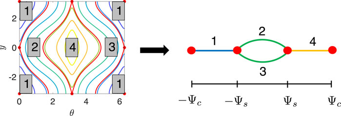
FIGURE 8. Reduction of the swimmer phase space to a graph. Each edge of the graph corresponds to the labeled region of phase space, and the nodes correspond to fixed points and separatrices at the boundaries of each region. Ψ is a coordinate along the edges of the graph.

To each edge, we associate a time-dependent probability density p_i (Ψ, τ), with i ∈ {1, 2, 3, 4}. The densities p_i evolve according to the Fokker-Planck equations associated with Eq. 23,

$\frac{\partial p_i}{\partial \tau }=-\frac{\partial }{\partial \mathrm{\Psi }}\left(f_i{p}_i\right)+\frac{{\partial }^2}{\partial {\mathrm{\Psi }}^2}\left(D_i{p}_i\right)=-\frac{\partial J_i}{\partial \mathrm{\Psi }},(24)$

where J_i is the probability current density

$J_i=f_i{p}_i-\frac{\partial }{\partial \mathrm{\Psi }}\left(D_i{p}_i\right).(25)$

In Eqs 24, 25, f_i and D_i are the averaged drifts and diffusions [Eqs 18, 21 respectively] evaluated in the regions of phase space corresponding to the edges of the graph in Figure 8. At the nodes of the graph where the islands and jets meet, the local conservation of probability implies that the total probability current density entering a node must equal the total probability current density leaving the node, similar to Kirchoff’s first law for circuits. To obtain the total probability current density entering (leaving) a node, one sums over the J_i for edges i connected to that node such that the node is approached in the direction of increasing (decreasing) Ψ. The boundary conditions are thus

$J_1\left(-{\mathrm{\Psi }}_s\right)=J_2\left(-{\mathrm{\Psi }}_s\right)+J_3\left(-{\mathrm{\Psi }}_s\right),(\mathrm{26a})$

$J_4\left({\mathrm{\Psi }}_s\right)=J_2\left({\mathrm{\Psi }}_s\right)+J_3\left({\mathrm{\Psi }}_s\right).(\mathrm{26b})$

Equations 24, 26 thus constitute a drift-diffusion process on the graph illustrated in Figure 8, which captures the swimmer dynamics in the σ → 0 limit.

In order to investigate the steady-state behavior of the swimmer in the weak-noise limit, we seek the steady-state solution of Eqs. 24–26. Because the jets are identical to each other by symmetry, f₂ = f₃ and D₂ = D₃ in Eq. 24, and therefore p₂ = p₃ must be satisfied in the steady-state. This allows us to merge the distinct p_i into a single steady-state density, p₀(Ψ), defined over the entire range −Ψ_c ≤ Ψ ≤ Ψ_c, which satisfies

$p_0\left(\mathrm{\Psi }\right)=\left\{\begin{array}{cc}{p}_1\hfill & \mathrm{f}\mathrm{o}\mathrm{r}-{\mathrm{\Psi }}_c\le \mathrm{\Psi }<-{\mathrm{\Psi }}_s,\hfill \\ p_2+p_3=2p_2\hfill & \mathrm{f}\mathrm{o}\mathrm{r}-{\mathrm{\Psi }}_s\le \mathrm{\Psi }<{\mathrm{\Psi }}_s,\hfill \\ p_4\hfill & \mathrm{f}\mathrm{o}\mathrm{r}{\mathrm{\Psi }}_s\le \mathrm{\Psi }\le {\mathrm{\Psi }}_c.\hfill \end{array}\right.(27)$

The density p₀ satisfies the steady-state Fokker-Planck equation

$-\frac{\mathrm{d}}{\mathrm{d}\mathrm{\Psi }}\left(f{p}_0\right)+\frac{{\mathrm{d}}^2}{\mathrm{d}{\mathrm{\Psi }}^2}\left(D{p}_0\right)=0.(28)$

Eq. 28 can be integrated once, which after rearrangement gives

$p_0^{\prime }=\frac{1}{D}\left[\left(f-D^{\prime }\right)p_0+C_1\right],(29)$

where C₁ is an integration constant and (⋅)′ ≡d(⋅)/dΨ. Eq. 29 is linear, and its solution is

$p_0\left(\mathrm{\Psi }\right)=\exp \left[{\int }_{-{\mathrm{\Psi }}_c}^{\mathrm{\Psi }}\frac{f\left({\mathrm{\Psi }}_1\right)-D^{\prime }\left({\mathrm{\Psi }}_1\right)}{D\left({\mathrm{\Psi }}_1\right)}\mathrm{d}{\mathrm{\Psi }}_1\right]\times \left\{C_0+C_1{\int }_{-{\mathrm{\Psi }}_c}^{\mathrm{\Psi }}\frac{\exp \left[-{\int }_{-{\mathrm{\Psi }}_c}^{{\mathrm{\Psi }}_1}\frac{f\left({\mathrm{\Psi }}_2\right)-D^{\prime }\left({\mathrm{\Psi }}_2\right)}{D\left({\mathrm{\Psi }}_2\right)}\mathrm{d}{\mathrm{\Psi }}_2\right]}{D\left({\mathrm{\Psi }}_1\right)}\mathrm{d}{\mathrm{\Psi }}_1\right\},(30)$

where C₀ is another integration constant. Due to the symmetry of the problem, the conditions

$p_0\left(-{\mathrm{\Psi }}_c\right)=p_0\left({\mathrm{\Psi }}_c\right),(\mathrm{31a})$

$f\left(\mathrm{\Psi }\right)=-f\left(-\mathrm{\Psi }\right),(\mathrm{31b})$

$D\left(\mathrm{\Psi }\right)=D\left(-\mathrm{\Psi }\right)(\mathrm{31c})$

must be satisfied. We substitute Eq. 30 into Eq. 31a, which gives

$C_0=C_0+C_1{\int }_{-{\mathrm{\Psi }}_c}^{{\mathrm{\Psi }}_c}\frac{\exp \left[-{\int }_{-{\mathrm{\Psi }}_c}^{{\mathrm{\Psi }}_1}\frac{f\left({\mathrm{\Psi }}_2\right)-D^{\prime }\left({\mathrm{\Psi }}_2\right)}{D\left({\mathrm{\Psi }}_2\right)}\mathrm{d}{\mathrm{\Psi }}_2\right]}{D\left({\mathrm{\Psi }}_1\right)}\mathrm{d}{\mathrm{\Psi }}_1,(32)$

where we have used Eqs 31b, 31c in evaluating the first term of Eq. 30 on the right-hand side of Eq. 31a. Eq. 32 implies C₁ = 0. Hence, the steady-state Ψ distribution has the form

$p_0\left(\mathrm{\Psi }\right)=\frac{C_0}{D\left(\mathrm{\Psi }\right)}\exp \left[{\int }_{-{\mathrm{\Psi }}_c}^{\mathrm{\Psi }}\frac{f\left({\mathrm{\Psi }}_1\right)}{D\left({\mathrm{\Psi }}_1\right)}\mathrm{d}{\mathrm{\Psi }}_1\right],(33)$

where we have absorbed another constant into C₀, which now plays the role of normalization constant. Eq. 33 is the invariant density of the reduced drift-diffusion model (23). Physically, it is the steady-state probability density of finding a swimmer on a deterministic trajectory with a particular constant of motion Ψ in the σ → 0 limit.

We now use p₀ to reconstruct the phase-space distribution P₀ (y, θ) that is obtained in the σ → 0 limit. The idea is to make a change of coordinates (y, θ)↦(Ψ, s), where Ψ = Ψ (y, θ) is defined by Eq. 6 and s = s (y, θ) is the elapsed Euclidean arclength along a trajectory at fixed Ψ, defined by

$\mathrm{d}s=\sqrt{\mathrm{d}{y}^2+\mathrm{d}{\theta }^2}=|\dot{\mathbf{\text{q}}}|\mathrm{d}t,(34)$

where q = (y, θ) and $|\dot{\mathbf{\text{q}}}|\equiv {({\dot{y}}^2+{\dot{\theta }}^2)}^{1/2}$. The coordinates (Ψ, s) are akin to action-angle variables in Hamiltonian mechanics. Note that this is a local rather than global change of coordinates, because for each value of Ψ in the jet region, there are two distinct orbits, one above and one below the separatrix (see Figure 8). Under this change of coordinates, the phase-space probability distribution must transform as

$\begin{array}{ll}\hfill P_0\left(y,\theta \right)\mathrm{d}y\mathrm{d}\theta & =P^{\ast }\left(\mathrm{\Psi },s\right)\mathrm{d}\mathrm{\Psi }\mathrm{d}s\hfill \\ \hfill & =P^{\ast }\left(\mathrm{\Psi },s\right)\left|\det \left[\frac{\partial \left(\mathrm{\Psi },s\right)}{\partial \left(y,\theta \right)}\right]\right|\mathrm{d}y\mathrm{d}\theta .\hfill \end{array}(35)$

Here, P^∗(Ψ, s) is the steady-state distribution in (Ψ, s) coordinates. Under the assumptions of the averaging principle, the fast motion along the s coordinate is decoupled from the slow motion along the Ψ coordinate, so the joint density P^∗(Ψ, s) must be the product of the density of the Ψ coordinate, p₀(Ψ), and the invariant density along an orbit of fixed Ψ. The latter is inversely proportional to the phase-space speed $|\dot{\mathbf{\text{q}}}|$ at each point. In addition, we must account for the fact that for values of Ψ in the jet region, the two jets share probability equally [see Eq. 27]. Therefore, we obtain

$P^{\ast }\left(\mathrm{\Psi },s\right)=\left\{\begin{array}{cc}\frac{p_0\left(\mathrm{\Psi }\right)}{T\left(\mathrm{\Psi }\right)|\dot{\mathbf{\text{q}}}|}\hfill & \mathrm{f}\mathrm{o}\mathrm{r}|\mathrm{\Psi }|>{\mathrm{\Psi }}_s,\hfill \\ \frac{1}{2}\frac{p_0\left(\mathrm{\Psi }\right)}{T\left(\mathrm{\Psi }\right)|\dot{\mathbf{\text{q}}}|}\hfill & \mathrm{o}\mathrm{t}\mathrm{h}\mathrm{e}\mathrm{r}\mathrm{w}\mathrm{i}\mathrm{s}\mathrm{e}.\hfill \end{array}\right.(36)$

The orbit period T is included in Eq. 36 to normalize the invariant density of the s coordinate.

The calculation of the determinant in Eq. 35 requires the partial derivatives of Ψ and s with respect to (y, θ). The partial derivatives of Ψ are straightforward to obtain from Eq. 6. The partial derivatives of s follow from Eq. 34,

$\frac{\mathrm{d}s}{\mathrm{d}t}=|\dot{\mathbf{\text{q}}}|=\nabla s\cdot \dot{\mathbf{\text{q}}},(37)$

where ∇ ≡ (∂/∂y, ∂/∂θ). From Eq. 37, it follows that

$\nabla s=\frac{\dot{\mathbf{\text{q}}}}{|\dot{\mathbf{\text{q}}}|}.(38)$

Thus, a straightforward calculation leads to

$\det \left[\frac{\partial \left(\mathrm{\Psi },s\right)}{\partial \left(y,\theta \right)}\right]=-\frac{2|\dot{\mathbf{\text{q}}}|}{1-\alpha \cos 2\theta }.(39)$

Combining Eqs 35, 36, 39, we finally obtain

$P_0\left(y,\theta \right)=\frac{g\left(\mathrm{\Psi }\left(y,\theta \right)\right)}{1-\alpha \cos 2\theta },(40)$

where

$g\left(\mathrm{\Psi }\right)=\left\{\begin{array}{cc}\frac{2p_0\left(\mathrm{\Psi }\right)}{T\left(\mathrm{\Psi }\right)}\hfill & \mathrm{f}\mathrm{o}\mathrm{r}|\mathrm{\Psi }|>{\mathrm{\Psi }}_s,\hfill \\ \frac{p_0\left(\mathrm{\Psi }\right)}{T\left(\mathrm{\Psi }\right)}\hfill & \mathrm{o}\mathrm{t}\mathrm{h}\mathrm{e}\mathrm{r}\mathrm{w}\mathrm{i}\mathrm{s}\mathrm{e}.\hfill \end{array}\right.(41)$

Eq. 40 shows that the nonuniformity of the steady-state probability density P (y, θ) in the limit of small noise results from two effects: rotational slowdown and noise-induced drift. Regardless of where one is in phase space, the density is modulated by the factor of (1 − α cos 2θ)⁻¹. This factor accounts for the slowdown of rotating elongated particles, caused by the orientation-dependent angular velocity in Eq. 3b. In addition to this, the density is modulated by the function g(Ψ), which weights each point (y, θ) according to the deterministic orbit it belongs to, indexed by Ψ (y, θ). The modulation by g accounts for the slow dynamics across the deterministic periodic orbits, encapsulated by the averaged drift-diffusion model (23).

4.2 Unraveling Density Variations and Depletion

We proceed by evaluating p₀(Ψ) through the numerical evaluation of Eqs 18, 21, 33 for selected parameters (v₀, α) [23]¹. The resulting distributions are compared against the distributions p(Ψ) obtained directly from the numerical solutions P (y, θ) to the Fokker-Planck Equation 12. We compute p(Ψ) using

$p\left(\mathrm{\Psi }\right)\approx \frac{1}{\mathrm{\Delta }\mathrm{\Psi }}{\int }_{\mathrm{\Psi }}^{\mathrm{\Psi }+\mathrm{\Delta }\mathrm{\Psi }}P\left(y,\theta \right)\mathrm{d}y\mathrm{d}\theta (42)$

for small ΔΨ. Example results are presented in Figure 9. Note that in each panel of Figure 9, p is plotted for the range −Ψ_c ≤ Ψ ≤ Ψ_c. Because Ψ_c depends on v₀ and α, the numerical ranges of p are different in each panel. For sufficiently small σ, we see excellent agreement between p₀ predicted by the averaging principle and p obtained from the exact solutions of the Fokker-Planck equation (Figures 9A,C,E,F). As the intensity of noise increases, the two Ψ distributions begin to deviate from each other, as seen when comparing Figures 9A,D. The assumption underlying the averaging principle is that the noise-induced drift across orbits is slow compared to the fast motion around the deterministic periodic orbits. We estimate the time scale of the fast motion using the period T (Ψ_c) of small oscillations around the centers (y, θ) = (0, π) and (π, 0), which is given by $T({\mathrm{\Psi }}_c)=2^{3/2}\pi /\sqrt{v_0(1-\alpha )}$. Meanwhile, the time scale of the noise-induced drift can be estimated as τ_noise = 1/σ² [see Eq. 16]. Hence, we expect good agreement between p₀ and p when τ_noise ≫ T (Ψ_c), which can be rearranged to give

${\sigma }^2\ll \frac{\sqrt{v_0\left(1-\alpha \right)}}{2^{3/2}\pi }.(43)$

FIGURE 9

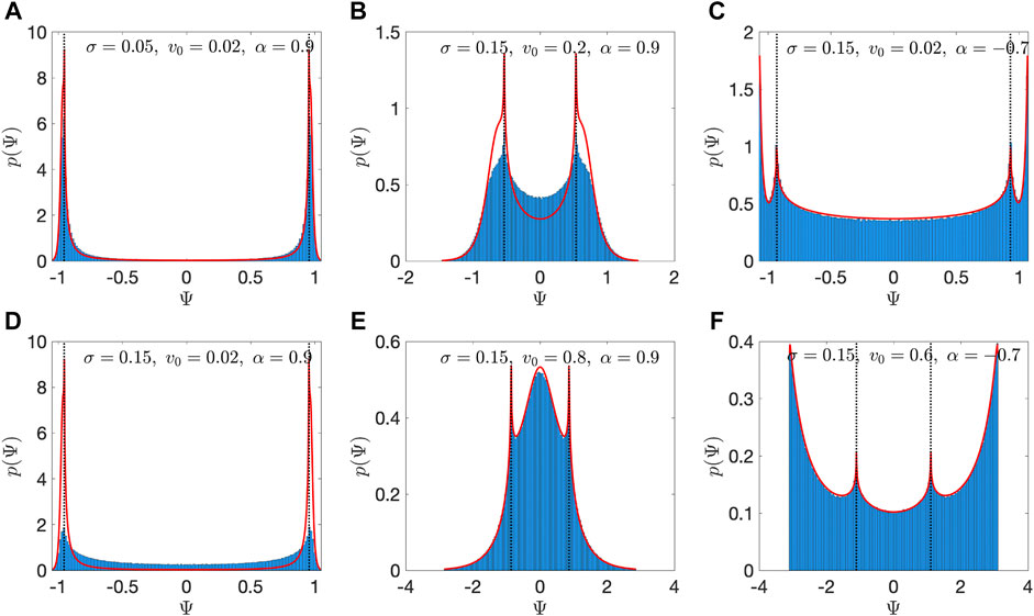
FIGURE 9. Comparison of the steady-state Ψ distributions from the averaging principle [p₀(Ψ), red curves] and those obtained from solving the Fokker-Planck Equation 12 and applying Eq. 42. The parameters are the same as in Figure 4. Panels A–D are for parameters before the bifurcation from rotational to cross-stream drift, and panels E and F are after this bifurcation. Black dotted lines indicate the Ψ values of the separatrices ±Ψ_s. Note that p₀(Ψ) does not depend on σ, so the curves plotted in panels (A) and (D) are the same.

Eq. 43 can also be expressed in terms of the dimensional quantities as

$\frac{D_{R}w}{\sqrt{VU\left(1-\alpha \right)}}\ll 1,(44)$

where we have dropped the numerical constants. The scaling behavior in Eq. 43 explains why for the same value of σ = 0.15, the agreement between p₀ and p is better for large v₀ (Figure 9E compared to Figures 9B,D) and α < 0 (Figure 9C compared to Figure 9D).

Next, we compare the probability densities P₀ predicted by the reduced model and given by Eq. 40 to the densities P obtained by solving the Fokker-Planck Equation 12. In particular, we focus on assessing the extent to which the non-uniformity of P is caused by noise-induced drift, as opposed to rotational slowdown. Owing to the form of P in the σ → 0 limit given in Eq. 40, we filter out the effect of rotational slowdown by multiplying the densities by 1 − α cos (2θ). The results are shown in Figure 10 for selected parameters. Figures 10A–C show Fokker-Planck densities P with the rotational slowdown modulation removed, and they correspond to Figures 4A,C,E, respectively. For α > 0 (Figures 10A,C), the peaks at θ = 0 and π are gone, confirming that these peaks are caused by rotational slowdown. Similarly, for α < 0 (Figure 10B), the peaks at θ = π/2 and 3π/2 are gone. Furthermore, the filtered densities P (1 − α cos 2θ) from the Fokker-Planck simulations (Figures 10A–C) agree well with the corresponding filtered densities P₀ (1 − α cos 2θ) obtained using the averaging technique in the weak-noise limit (Figures 10D–F). After filtering out the rotational slowdown, all that remains in P₀ is g (Ψ(y, θ)). Thus, Figures 10D–F display the orbit weight-factor g at each point of phase space.

FIGURE 10

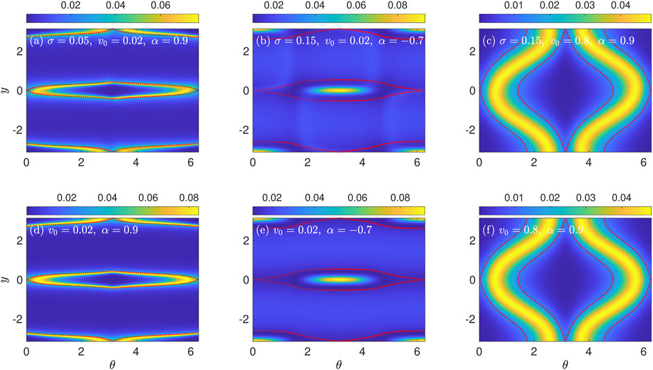
FIGURE 10. Comparison of (A–C) the phase-space distributions with the rotational slowdown effect filtered out, P (y, θ) (1 − α cos 2θ), with (D–F) the distributions P₀ (y, θ) (1 − α cos 2θ) predicted by the averaging model given in Eq. 40.

Figure 11 shows g(Ψ) for several representative combinations of v₀ and α. Note that g(Ψ) appears to be a smooth function, while p₀(Ψ) possesses singularities at the separatrices Ψ = ±Ψ_s, as seen in Figure 9. It can be shown that these singularities occur because in Eq. 33, D (±Ψ_s) = 0. However, from Eq. 41 we have g ∝ p₀/T, and T also diverges at the separatrices. Evidently, these singularities exactly cancel each other out, making g a smooth function.

FIGURE 11

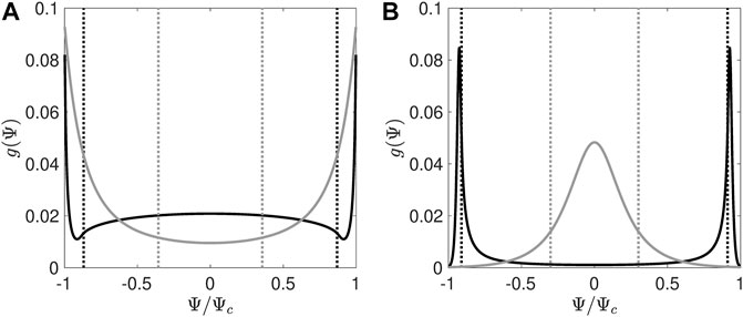
FIGURE 11. Phase space weight factors g for (A) α = − 0.7 and (B) α = 0.9. The solid curves are g(Ψ), and the dotted curves represent the separatrices at ±Ψ_s. Different shades represent different swimming speeds v₀. (A) Black is v₀ = 0.02, and grey is v₀ = 0.6. (B) Black is v₀ = 0.02, and grey is v₀ = 0.8.

The good agreement between Figures 10A–F both validates the reduced model derived in Sec. 4.1 and shows the importance of noise-induced drift in shaping the overall phase-space densities. In particular, the shape of g(Ψ) for different values of swimmer speed v₀ and shape α explains many of our observations concerning the steady-state distributions P (y, θ) in Sec. 3. For example, for α < 0, g is always peaked at the boundaries ±Ψ_c (Figure 11A). In phase space, these features manifest as peaks on the centers, as seen in Figures 10B,E, as well as Figures 4C,F. When v₀ is sufficiently small, g also has a secondary, broad peak centered on the jet region (Ψ = 0), as evidenced by the black curve (v₀ = 0.02) in Figure 11A. This leads to a significant density in the jet regions, as seen in Figure 4C. As v₀ increases, the height of this secondary peak relative to the peaks at ±Ψ_c decreases, while the local minima on either side of the central peak creep inward. For sufficiently large v₀, these local minima merge and the secondary peak disappears entirely, as evidenced by the grey curve (v₀ = 0.6) in Figure 11A. Thus, as v₀ grows, the orbits in the jet region become increasingly suppressed for α < 0 swimmers (Figure 4F).

We observe qualitatively different behavior for g when α > 0 (Figure 11B). When v₀ is small, g is always peaked near the separatrices, as illustrated by the black curve (v₀ = 0.02) in Figure 11B. Note that the peaks are slightly offset from the separatrices, shifted towards the islands. This feature explains the bright bands just inside the separatrices seen in the filtered P (y, θ) distributions in Figures 10A,D and the raw distributions in Figures 4A,B,D. As v₀ increases, both the separatrices and the peaks of g move inward towards Ψ = 0. For sufficiently large v₀, these peaks merge and g exhibits a single peak at Ψ = 0, as illustrated by the grey curve (v₀ = 0.8) in Figure 11B. Hence, at sufficiently high v₀, the orbits in the jet region are weighted the highest, as seen in Figures 10C,F.

The variation of g with the swimmer parameters also clarifies the variation of the depletion index I_D as a function of v₀ and α. Figure 12A shows the variation of I_D predicted using P₀ given by Eq. 40. The quantitative agreement with the depletion index from the Fokker-Planck model is excellent for σ = 0.05 (Figure 12B) and reasonable for σ = 0.15 (Figure 12C). For α < 0, we can now ascribe the transition from low-to high-shear depletion (positive to negative I_D) to the increasing dominance of the peaks of g at Ψ = ±Ψ_c as v₀ increases. Meanwhile, for α > 0, we ascribe the transition from high-to low-shear depletion to the peaks of g tracking the separatrices, which narrowly hug the centerlines for small v₀ and gradually widen as v₀ increases.

FIGURE 12

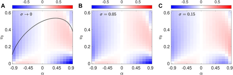
FIGURE 12. Depletion index I_D as a function of (v₀, α) for fixed values of σ. (A) σ → 0, using the averaged drift-diffusion model and Eq. 40. The black dotted curve is the bifurcation curve from Figure 3. (B) σ = 0.05, from the Fokker-Planck model. (C) σ = 0.15, from the Fokker-Planck model.

As for the second transition to high-shear depletion that occurs for α > 0 as v₀ increases further, i.e., the blue region in the upper-right corner of Figure 12A, this is actually due to the interplay between noise-induced drift and rotational slowdown. To demonstrate this, in Figure 13 we compare I_D calculated using the full P₀ given by Eq. 40 (Figure 13A) to a calculation of I_D where we use instead the filtered density P₀ (y, θ) (1 − α cos 2θ) = g (Ψ(y, θ)), which must be normalized (Figure 13B). The two calculations agree well everywhere except for α near 1 for high v₀. In that region, I_D decreases as v₀ increases in both cases, but with rotational slowdown included (Figure 13A), the decline of I_D is enhanced to the point that it becomes negative. For α near 1 and high v₀, g is peaked at Ψ = 0 (Figure 11B), so that orbits in the jet region are highly weighted (Figures 10C,F). At the same time, the rotational slowdown factor 1 − α cos 2θ is accentuated, due to a larger |α|. The combination of these two effects leads to a very high concentration of P (y, θ) near the saddles, modest ridges in the jet regions, and a steep drop-off everywhere else, as seen in Figure 4E. These elements combined then lead to I_D < 0. Overall, we conclude that noise-induced drift is the dominant effect underlying the (v₀, α) parameter dependence of I_D, while rotational slowdown is a secondary effect that becomes most important for fast and highly elongated α > 0 swimmers.

FIGURE 13

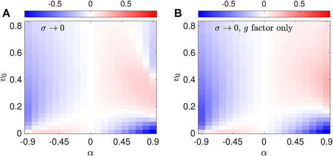
FIGURE 13. Comparison of calculations of the depletion index I_D (A) using P₀ (y, θ) vs. (B) using the rotational slowdown filtered P₀ (1 − α cos 2θ) = g.

5 Conclusion

To conclude, we have analyzed the distribution of microswimmers in the planar, laminar Kolmogorov flow. These distributions are highly nonuniform for elongated swimmers, and the swimmer concentration may be depleted from either low- or high-shear regions of the flow [1, 10]. To explain this effect, we derived a reduced model using an averaging technique [25], which captures the slow motion of swimmers transverse to the deterministic orbits that is induced by weak diffusion. The model leads to an invariant density on the space of deterministic swimmer orbits, parametrized by the constant of motion Ψ of the deterministic dynamics. The steady-state phase-space densities predicted by the reduced model are in good agreement with those obtained from the original model, showing that the main cause of depletion is the noise-induced drift of swimmers in phase space.

The averaging technique we employed here can be applied to other problems involving noisy self-propelled particles in fluid flows. For systems with an effectively two-dimensional phase space, the technique is applicable so long as the system possesses a conserved quantity and the noise is diffusive. For example, it may also be applied to gyrotactic swimmers in a planar laminar Kolmogorov flow [14] and swimmers with both translational and rotational diffusion [19, 22]. For higher dimensional systems possessing one or multiple conserved quantities, such as swimmers in three-dimensional channel flows [13], a generalization of the two-dimensional theory exists for extracting the slow dynamics induced by weak noise [25]. While we focused here on a steady flow, the averaging technique could potentially be generalized to an unsteady flow with simple time dependence. Even though we do not expect a conserved quantity in that case, it is possible that there is a fast time scale of the motion that can be averaged out in a similar fashion. It is also an open question whether an averaging approach would be applicable to models where the rotational noise of the swimmer contains a tumbling component in addition to (or instead of) rotational diffusion [22, 26, 27].

The simplicity of swimmer motion in the Kolmogorov flow makes it a good testbed for understanding other aspects of swimmer-flow interaction. For example, it could be used to better understand the effects of chemotaxis on density variations of swimming microorganisms in fluid flows [1, 26, 27]. Our model can be modified by making the noise intensity σ vary with y and θ, in order to mimic the position- and orientation-dependent tumbling rate of chemotactic swimming bacteria in response to a chemical gradient in the flow. This would modify the averaged drift and diffusion functions f and D, defined in Eqs 18, 21, and it would potentially break the symmetry between the two distinct jet regions. However, the rest of the procedure carried out in Sec. 4 would still be applicable.

Finally, it may be possible to exploit the parameter dependence of the density of variations of swimmers in the Kolmogorov flow to sort particles with differing properties.

Data Availability Statement

The original contributions presented in the study are included in the article/Supplementary Material, further inquiries can be directed to the corresponding authors.

Author Contributions

SB conceived and designed the research. SB, KF, and NB performed the analytical and numerical calculations. All authors contributed to the interpretation of the results and data. SB wrote the first draft of the manuscript. All authors contributed to the revision of the manuscript.

Funding

This study was supported by the National Science Foundation under grants CMMI-1825 379 and DMR-1806 355.

Conflict of Interest

The authors declare that the research was conducted in the absence of any commercial or financial relationships that could be construed as a potential conflict of interest.

Publisher’s Note

All claims expressed in this article are solely those of the authors and do not necessarily represent those of their affiliated organizations, or those of the publisher, the editors and the reviewers. Any product that may be evaluated in this article, or claim that may be made by its manufacturer, is not guaranteed or endorsed by the publisher.

Supplementary Material

The Supplementary Material for this article can be found online at: https://www.frontiersin.org/articles/10.3389/fphy.2021.816663/full#supplementary-material

Footnotes

¹Github Our code used to solve the Fokker Planck equation and compute the quantities associated with the averaged drift-diffusion model (2021) Available at: https://github.com/saberman52/KolmogorovFlowSwimmerDynamics. (Acccessed: December 3, 2021).

References

1. Rusconi R, Guasto JS, Stocker R Bacterial Transport Suppressed by Fluid Shear. Nat Phys (2014) 10:212–7. doi:10.1038/nphys2883

CrossRef Full Text | Google Scholar

2. Ebbens SJ, Howse JR In Pursuit of Propulsion at the Nanoscale. Soft Matter (2010) 6:726–38. doi:10.1039/b918598d

CrossRef Full Text | Google Scholar

3. Bechinger C, Di Leonardo R, Löwen H, Reichhardt C, Volpe G, Volpe G Active Particles in Complex and Crowded Environments. Rev Mod Phys (2016) 88:045006. doi:10.1103/RevModPhys.88.045006

CrossRef Full Text | Google Scholar

4. Sanchez T, Chen DTN, Decamp SJ, Heymann M, Dogic Z Spontaneous Motion in Hierarchically Assembled Active Matter. Nature (2012) 491:431–4. doi:10.1038/nature11591

PubMed Abstract | CrossRef Full Text | Google Scholar

5. Torney C, Neufeld Z Transport and Aggregation of Self-Propelled Particles in Fluid Flows. Phys Rev Lett (2007) 99:078101. doi:10.1103/PhysRevLett.99.078101

PubMed Abstract | CrossRef Full Text | Google Scholar

6. Khurana N, Blawzdziewicz J, Ouellette NT Reduced Transport of Swimming Particles in Chaotic Flow Due to Hydrodynamic Trapping. Phys Rev Lett (2011) 106:198104. doi:10.1103/PhysRevLett.106.198104

PubMed Abstract | CrossRef Full Text | Google Scholar

7. Berman SA, Mitchell KA Trapping of Swimmers in a Vortex Lattice. Chaos (2020) 30:063121. doi:10.1063/5.0005542

PubMed Abstract | CrossRef Full Text | Google Scholar

8. Ariel G, Schiff J Conservative, Dissipative and Super-diffusive Behavior of a Particle Propelled in a Regular Flow. Physica D: Nonlinear Phenomena (2020) 411:132584. doi:10.1016/j.physd.2020.132584

CrossRef Full Text | Google Scholar

9. Berman SA, Buggeln J, Brantley DA, Mitchell KA, Solomon TH Transport Barriers to Self-Propelled Particles in Fluid Flows. Phys Rev Fluids (2021) 6:L012501. doi:10.1103/PhysRevFluids.6.L012501

CrossRef Full Text | Google Scholar

10. Barry MT, Rusconi R, Guasto JS, Stocker R Shear-induced Orientational Dynamics and Spatial Heterogeneity in Suspensions of Motile Phytoplankton. J R Soc Interf (2015) 12:20150791. doi:10.1098/rsif.2015.0791

CrossRef Full Text | Google Scholar

11. Vennamneni L, Nambiar S, Subramanian G Shear-induced Migration of Microswimmers in Pressure-Driven Channel Flow. J Fluid Mech (2020) 890:A15. doi:10.1017/jfm.2020.118

CrossRef Full Text | Google Scholar

12. Zöttl A, Stark H Nonlinear Dynamics of a Microswimmer in Poiseuille Flow. Phys Rev Lett (2012) 108:218104. doi:10.1103/PhysRevLett.108.218104

PubMed Abstract | CrossRef Full Text | Google Scholar

13. Zöttl A, Stark H Periodic and Quasiperiodic Motion of an Elongated Microswimmer in Poiseuille Flow. Eur Phys J E (2013) 36:4. doi:10.1140/epje/i2013-13004-5

CrossRef Full Text | Google Scholar

14. Santamaria F, De Lillo F, Cencini M, Boffetta G Gyrotactic Trapping in Laminar and Turbulent Kolmogorov Flow. Phys Fluids (2014) 26:111901. doi:10.1063/1.4900956

CrossRef Full Text | Google Scholar

15. Arguedas-Leiva J-A, Wilczek M Microswimmers in an Axisymmetric Vortex Flow. New J Phys (2020) 22:053051. doi:10.1088/1367-2630/ab776f

CrossRef Full Text | Google Scholar

16. Chen H, Thiffeault J-L Shape Matters: A Brownian Microswimmer in a Channel. J Fluid Mech (2021) 916:A15. doi:10.1017/jfm.2021.144

CrossRef Full Text | Google Scholar

17. Jeffery GB. The Motion of Ellipsoidal Particles Immersed in a Viscous Fluid. Proc R Soc Lond A (1922) 102:161–79. doi:10.1098/rspa.1922.0078

CrossRef Full Text | Google Scholar

18. Strogatz SH. Nonlinear Dynamics and Chaos: With Applications to Physics, Biology, Chemistry, and Engineering. Boca Raton: CRC Press (2018).

Google Scholar

19. Thiffeault JL, Guo J. Shake Your Hips: An Anisotropic Active Brownian Particle with a Fluctuating Propulsion Force. (2021) arXiv:2102.11758 [cond–mat.soft].

Google Scholar

20. Hyon Y, Marcos, , Powers TR, Stocker R, Fu HC The Wiggling Trajectories of Bacteria. J Fluid Mech (2012) 705:58–76. doi:10.1017/jfm.2012.217

CrossRef Full Text | Google Scholar

21. Solon AP, Cates ME, Tailleur J Active Brownian Particles and Run-And-Tumble Particles: A Comparative Study. Eur Phys J Spec Top (2015) 224:1231–62. doi:10.1140/epjst/e2015-02457-0

CrossRef Full Text | Google Scholar

22. Berman SA, Mitchell KA Swimmer Dynamics in Externally-Driven Fluid Flows: The Role of Noise (2021) arXiv:2108.10488 [physics.flu-dyn].

Google Scholar

23.Github Our code used to solve the Fokker Planck equation and compute the quantities associated with the averaged drift-diffusion model (2021) Available at: https://github.com/saberman52/KolmogorovFlowSwimmerDynamics. (Acccessed: December 3, 2021).

Google Scholar

24. Hassler U. Stochastic Processes and Calculus. Cham: Springer (2016).

Google Scholar

25. Freidlin MI, Wentzell AD. Random Perturbations of Dynamical Systems. New York, NY: Springer (2012). doi:10.1007/978-3-642-25847-3

CrossRef Full Text | Google Scholar

26. Locsei JT, Pedley TJ Run and Tumble Chemotaxis in a Shear Flow: The Effect of Temporal Comparisons, Persistence, Rotational Diffusion, and Cell Shape. Bull Math Biol (2009) 71:1089–116. doi:10.1007/s11538-009-9395-9

PubMed Abstract | CrossRef Full Text | Google Scholar

27. Bearon RN, Hazel AL The Trapping in High-Shear Regions of Slender Bacteria Undergoing Chemotaxis in a Channel. J Fluid Mech (2015) 771:R3. doi:10.1017/jfm.2015.198

CrossRef Full Text | Google Scholar