Nonreversible Markov Chain Monte Carlo Algorithm for Efficient Generation of Self-Avoiding Walks

We introduce an efficient nonreversible Markov chain Monte Carlo algorithm to generate self-avoiding walks with a variable endpoint. In two dimensions, the new algorithm slightly outperforms the two-move nonreversible Berretti-Sokal algorithm introduced by H. Hu, X. Chen, and Y. Deng, while for three-dimensional walks, it is 3–5 times faster. The new algorithm introduces nonreversible Markov chains that obey global balance and allow for three types of elementary moves on the existing self-avoiding walk: shorten, extend or alter conformation without changing the length of the walk.

1 Introduction

A Self-Avoiding Walk (SAW) is defined as a contiguous sequence of moves on a lattice that does not cross itself; it does not visit the same point more than once. SAWs are fractals with fractal dimension 4/3 in two dimensions, close to 5/3 in three dimensions, and two in dimensions above four [2, 3]. In particular two-dimensional SAWs are conjectured to be the scaling limit of a family of random planar curves given by the Schramm-Loewner evolution with parameter κ = 8/3 [4]. Since their introduction, SAWs have been used to model linear polymers [5–7]. They are essential for studies of polymer enumeration where scaling theory, numerical approaches, and field theory are too hard to analyse [8, 9]. SAWs are also used in the numerical studies of finite-scaling [10] and two-point functions [11] of Ising model and n − vector spin model [12]. Analytical results on SAWs are scarce, and generating long SAWs is computationally complex.

Typically one uses Monte Carlo approaches [13, 14] to generate SAWs numerically. Many previous Markov chain Monte Carlo (MCMC) algorithms have been designed to efficiently produce different kinds of SAWs by manipulating potential constructions that can be executed on a walk to increase, decrease its length, or change its conformation. For example, the pivot algorithm samples fixed-length SAWs—it alters the walk’s shape without changing its length [15]. While the Berretti-Sokal algorithm and BFACF algorithm contain length-changing moves and can generate walks with varying lengths [16, 17].

The above described MCMC algorithms satisfy the detailed balance condition—which states that the weighted probabilities of transitions between states are equal. In other words, these algorithms use reversible Markov chains. The reversibility introduces a diffusion-like behavior in the space of states. In recent years, there has been progress in designing nonreversible Markov chains that converge to the correct target distribution. Such chains due to “inertia” reduce the diffusive behavior, sometimes leading to better convergence and mixing properties compared to the reversible chains [18–25].

As for SAW, H. Hu, X. Chen, and Y. Deng modified the Berretti-Sokal algorithm to allow for nonreversible Markov chains [1]. This modification yields about a ten times faster convergence than the original Berretti-Sokal algorithm in two dimensions and is even more superior in higher dimensions. Both the original and the modified Berretti-Sokal algorithm have two elementary moves—to shorten or extend the SAW. Building upon these algorithms, we add another move—to alter the conformation of SAW and introduce a three-move nonreversible MCMC technique to create SAWs. We discuss the advantages of this approach and compare the two nonreversible algorithms. The three types of moves correspond to three types of “atmospheres”; therefore, we start below by defining an atmosphere.

2 The Atmospheres

The algorithms creating SAWs usually manipulate different kinds of proposed moves, often referred to as atmospheres [26–29]. Atmospheres can be described as potential constructions that can be executed on a given walk to increase or decrease the current length or change the conformation. When generating SAWs, the algorithm usually performs moves on either endpoint atmospheres or generalized atmospheres where positive and negative atmospheres are generally defined as ways of adding or removing a fixed number of edges to the current walk. In contrast, neutral moves are ways of altering the walk’s shape without changing its length. For instance, the pivot algorithm, which only acts on neutral atmospheres, can be used to sample fixed-length walks [15]. In contrast, the Berretti-Sokal algorithm and BFACF algorithm contain length-changing atmospheric moves and can generate walks of different lengths [16, 17].

Suppose s is the current SAW starting from the origin with length |s| and its last vertex is v. The positive endpoint atmospheres are the lattice edges incident with the last vertex, which can be occupied to extend the length by one. The negative endpoint atmosphere is just the last occupied edge since removing it can extract the length by one. The neutral endpoint atmospheres are edges that can be occupied by changing the direction of the vertex v. For any SAW with a non-zero length, the number of negative endpoint atmospheres is one. If the SAW has zero length, the number of negative endpoint atmospheres is set to zero, as the length can not be further reduced.

Figure 1 shows a SAW with a length equal to four. In this example, three unoccupied edges are incident with the last vertex; they are shown in red on the graph, making three positive ending atmospheres. As we see from the last occupied edge (black arrow), there is just one negative endpoint atmosphere. There are two neutral endpoint atmospheres, and the corresponding edges are displayed with green arrows.

FIGURE 1

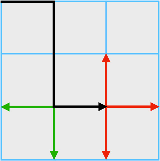
FIGURE 1. The endpoint atmospheres on a self-avoiding walk of length |s| = 4. For this self-avoiding walk, there are three positive ending atmospheres (red arrows) and one endpoint atmosphere, which is the last occupied edge (black arrow), and the number of neutral endpoint atmospheres is two (green arrows).

Three types of elementary moves in the algorithm executing the endpoint atmospheres correspond to the three kinds of endpoint atmospheres. Here we call a positive move the one to be performed on a positive endpoint atmosphere, resulting in occupying one empty edge incident with the last vertex. Similarly, a negative move implies executing on the negative endpoint atmosphere, that is, deleting the last occupied edge. Finally, the neutral move is changing the direction of the last occupied edge. The three kinds of moves’ for the SAW in Figure 1 are illustrated in Figure 2.

FIGURE 2

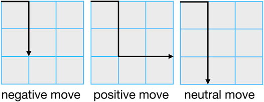
FIGURE 2. Possible self-avoiding walks after executing one move on the self-avoiding walk shown in Figure 1.

3 The Berretti-Sokal Algorithm

The balance condition is one of the most important factors in designing an MCMC algorithm since it ensures that the Markov chain will converge to a target distribution. The balance condition for most MCMCs is the so-called Detailed Balance Condition (DBC)

$P_{ij}{\pi }_j=P_{ji}{\pi }_i,\forall i,j\in \mathrm{\Omega },(1)$

where P_ij is the transition probability from state j to state i, Ω is the space of states, and π is the stationary distribution, see e.g., [21, 30]. Detailed balance is a local condition and thus easy to implement. However, for a Markov chain to asymptotically converge to a stationary distribution π, all we need is a weaker condition—the Global Balance Condition (GBC):

$\sum _{j\in \mathrm{\Omega }}{P}_{ij}{\pi }_j=\sum _{j\in \mathrm{\Omega }}{P}_{ji}{\pi }_i,\forall i\in \mathrm{\Omega },(2)$

where Ω is a space of states. The GBC physically means that the total probability influx at a state equals the total probability efflux from that state [13, 20].

Note that the probability distribution of a SAW of length |s| is

$\pi =x^{|s|}(3)$

where x is the weight of a unit step. This is what we want the Markov chain target distribution to be.

One of the most famous reversible MCMC algorithms that manipulate the endpoint atmospheres is the Berretti-Sokal algorithm [16]. The Berretti-Sokal algorithm only considers the positive and negative endpoint atmospheres and thus has two elementary moves: the increasing and the decreasing move. In this paper, we are using a Metropolis-Hastings style [31, 32] implementation of the Berretti-Sokal algorithm. It works as follows:

1) Suppose the current length of a SAW is given by N. With equal probability, the algorithm chooses the increasing move or the decreasing move.

2) If the increasing move is selected, with probability P₊ one of the empty edges incident with v_N, the last vertex, will be occupied randomly when this leads to a valid SAW of N + 1 steps. Similarly, for the decreasing move, the last occupied edge is deleted with probability P₋. The two probabilities are given by

$P_{+}=\min \left\{1,x\left(z-1\right)\right\},(4)$

$P_{-}=\min \left\{1,\frac{1}{x\left(z-1\right)}\right\},(5)$

where z is the coordination number of the system, i.e., the number of lattice points neighboring a vertex on the lattice.

Special attention is needed for the “null” walk, |s| = 0, in such case only an increasing mode is allowed and the number of empty edges is z, rather than z − 1. For simplicity we permanently set P₊ = min{1, x (z − 1)}.

To prove that the DBC holds in the Berretti-Sokal algorithm, let us for example consider the case where x (z − 1) < 1. From Eqs. 4, 5 we conclude that the choice implies P₊ < 1 and P₋ = 1. Thus we have x^|s|P₊(z − 1)⁻¹ = x^|s+1| = x^|s+1|P₋, which satisfies the DBC, given in Eq. 1. The proof is analogous in the case x (z − 1) > 1.

4 Nonreversible Berretti-Sokal Algorithms

One possible way to set up a nonreversible algorithm is to increase the phase space by introducing replicas [1, 20, 21] and work on the extended space with nonzero probability fluxes. Here we follow an analogous approach. As mentioned above, there has been a successful two-move nonreversible Berretti-Sokal algorithm [1]. The authors achieved an important improvement in the speed of the algorithm. The speedup is about tenfold in two-dimensional systems and is even more pronounced in higher-dimensional systems. They set up two modes in the algorithm, which we call the increasing mode and the decreasing mode.

4.1 Three-Move Nonreversible Berretti-Sokal Algorithm

The new algorithm has a third type of move—besides shortening and extending the SAW, we also allow the SAW to change its conformation. Namely, in the increasing mode, the algorithm can perform either an increasing move or a neutral move; in this mode, the decreasing move is not allowed. Analogously, in the decreasing mode, the algorithm will only execute either a decreasing move or a neutral move. A diagram describing the algorithm is shown in Figure 3. It works as follows:

1) In the increasing mode, with equal probability, perform either the positive move or the neutral move. For the positive move, the algorithm will randomly occupy one of the empty edges incident to the last vertex with probability P₊. While for the neutral move, the algorithm will change the direction of its last occupied edge randomly. If the chosen move does not lead to a valid SAW, the algorithm will change to the decreasing mode.

2) In the decreasing mode, with equal probability, perform either the negative move or the neutral move. For the negative move, the algorithm will delete the last occupied edge with probability P₋. For the neutral move, the algorithm will change the direction of its last occupied edge randomly. If the chosen move does not lead to a valid SAW, the algorithm will change into the increasing mode.

3) When the length is 0, the algorithm will be changed into the increasing mode, and a positive move will be performed.

FIGURE 3

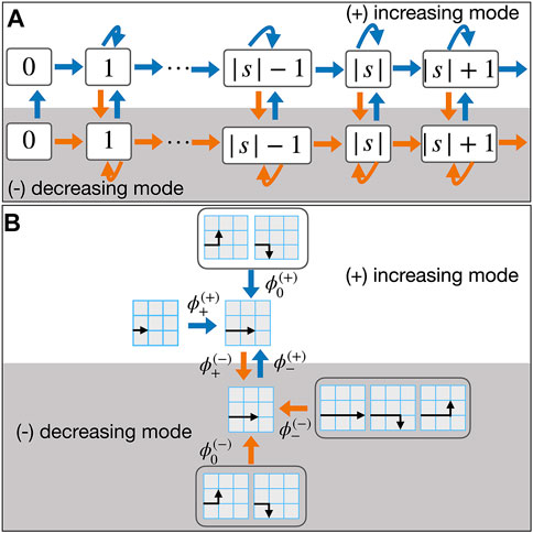
FIGURE 3. (A) Diagram of probability flows in the three-move nonreversible Berretti-Sokal algorithm. Each rectangle specifies a SAW of length |s|. Each realization of the algorithm is different because of the neutral moves, allowing to alter the configuration of the walk. The top row represents the increasing mode in which the algorithm can produce either a positive or neutral move, while the bottom row represents the decreasing mode where the algorithm produces either negative or neutral moves. The circular arrow represents the execution of a neutral move, leading to a SAW with the same length but a different shape as the last occupied edge’s direction is changed. The “null” walk, |s| = 0, requires special attention; in this case, we do not allow neutral and decreasing moves. (B) Example of the incoming fluxes for SAW of length |s| = 2 in 2D on a square lattice.

Therefore, in each step, the algorithm will either execute one of the elementary moves successfully or change to the other mode. The global balance condition implies that the total influx probability flow equals the efflux probability flow; that is, we have

${\varphi }_{\pm }^{\left(\pm \right)}+{\varphi }_0^{\left(\pm \right)}+{\varphi }_{\mp }^{\left(\pm \right)}=x^{|s|},(6)$

where x^|s| is the distribution of SAWs of length |s| and ϕ − s describe the incoming probability fluxes, where the superscript denotes the mode and the subscripts denote the move. The three terms on LHS are the incoming flow of executing a ± move in mode (±), ${\varphi }_{\pm }^{(\pm )}$, the incoming flow of executing one neutral move in mode (±), ${\varphi }_0^{(\pm )}$, and the incoming flow from switching the mode from (∓) to (±), ${\varphi }_{\mp }^{(\pm )}$. To clarify the third term in the LHS by example: ${\varphi }_{-}^{(+)}$ is the incoming flux from switching from (−) mode to the (+) mode. Let us show that global balance condition holds for the increasing mode when x (z − 1) < 1. Proofs for the other cases follow analogously. In this case the three fluxes are:

• The incoming flux from a positive move is

${\varphi }_{+}^{\left(+\right)}=x^{|s|-1}{P}_{+}\frac{1}{2\left(z-1\right)}=\frac{x^{|s|}}{2},(7)$

where in the second equality we used Eq. 4. The factor 1/2 is the result of selecting either a positive move or a neutral move and the term (z − 1)⁻¹ is from occupying one of the z − 1 empty edges incident to the last vertex.

• The incoming flux from a neutral move is

${\varphi }_0^{\left(+\right)}=\frac{x^{|s|}{z}^{″}}{2\left(z-1\right)},(8)$

where z^″ is the number of possible edges which will lead to a valid SAW for the last occupied edge when changing its direction.

• The incoming flux from the decreasing mode, ${\varphi }_{-}^{(+)}$, since P₋ = 1, as we assume that x (z − 1) < 1, the only possible reason of changing from another mode is that when the last occupied changes it direction, it does not lead to a valid SAW, thus

${\varphi }_{-}^{\left(+\right)}=\frac{1}{2}{x}^{|s|}\left(1-\frac{z^{″}}{z-1}\right).(9)$

Summing over the incoming flows, given in Eqs. 7–9 incoming-flow-from-minus, we verify that the global balance condition, Eq. 6, holds. Note that we do not assume that a particular SAW configuration of length |s| is achieved with the same frequency in the increasing and the decreasing mode—it comes out as a corollary of the global balance condition.

To test the efficiency of the new algorithm, we used the integrated autocorrelation time τ. For a given observable $\mathcal{O}$, it is defined as

$\tau =\frac{m}{2}\frac{{\sigma }_{\bar{\mathcal{O}}}^2}{{\sigma }_{\mathcal{O}}^2},(10)$

where m is the number of steps, $\bar{\mathcal{O}}$ is the estimator of the average $\mathcal{O}$, and σ² denotes a variance, c.f. [33]. Here we choose the length of the walk, |s|, for the observable as it is a common choice for SAWs. We tested the efficiency as a function of the linear system size by generating SAWs in a square lattice with n × n points and in a cubic lattice with n × n × n points. The boundary conditions were fixed. With τ₀ we denote the integrated autocorrelation time of the two-move nonreversible Berretti-Sokal algorithm (algorithm from [1]). The comparison of the two algorithms is on Figure 4.

FIGURE 4

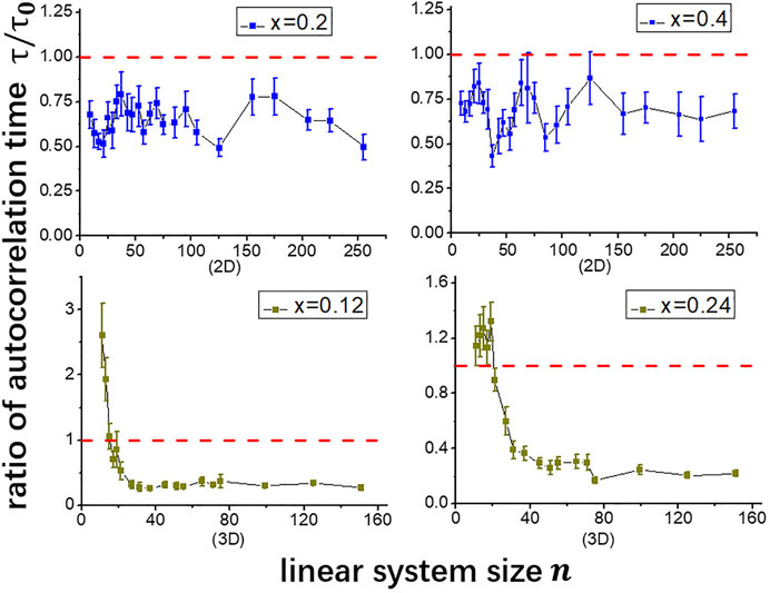
FIGURE 4. The ratio of integrated autocorrelation times of the three-move nonreversible Berretti-Sokal algorithm, τ, and the two-move nonreversible Berretti-Sokal algorithm, τ₀, for 2D, and 3D systems as a function of the linear system size n. The three-move nonreversible Berretti-Sokal algorithm’s performance is slightly better in 2D systems while it is 3 – 5 times faster in most 3D systems.

Note, that there are two different scenarios based on the value of weight of a unit step x. For example, for a 2D square lattice, when x = 0.4, P₊ = 1, and P₋ < 1, while for x = 0.2, P₋ = 1, and P₊ < 1. To study both scenarios present the results under initial setting where x = 0.2 and x = 0.4 in a 2D system and correspondingly x = 0.12 and x = 0.24 in a 3D system. From Figure 4 we conclude that the ratio of the autocorrelation times for large systems is weakly dependent on the value of x.

In 2D, the ratio of the autocorrelation time of the new algorithm over the previous one is always less than one, which means that the new algorithm has a slightly better performance. We further tested the new algorithm in a three-dimensional cubic system. The new algorithm tends to have better performance in large systems, and the difference is more significant than the 2D situation. When the length of the cube is less than 20, the previous algorithm is more efficient with less autocorrelation time. However, as the system’s scale increases, the ratio τ/τ₀ becomes less than one, and the value is between 0.2 and 0.3, indicating that the new algorithm is 3–5 times faster in these larger 3D systems. We have also tested our algorithm in 4D and 5D systems where no general improvements are found compared to the two-move nonreversible Berretti-Sokal algorithm. We show the detailed findings in Appendix. The fact that the addition of neutral moves does not improve the efficiency in generating SAWs in 4D and 5D, could be explained by the fact that as dimension gets higher, it will be much more likely for the algorithm to make a successful, positive move, which results in less benefit from adding the neutral move.

To summarize, we have created a new nonreversible algorithm manipulating the endpoint atmospheres to generate SAWs. By introducing all three kinds of endpoint atmospheres’ moves, the new algorithm has greater flexibility than the two-move nonreversible Berretti-Sokal algorithm, from [1]. For instance, when occupied lengths surround the endpoint of a given SAW, the algorithm will change into the negative mode since neither a neutral move nor a positive move will lead to a valid SAW. Assume that P₊ < 1, for an algorithm with only positive and negative moves, it will return to the origin and start from the beginning again. On the other hand, with a neutral move, the SAW does not have to start from the origin again. When a neutral move in the negative mode is not possible, the algorithm will change into the positive mode. The addition of neutral moves gives the algorithm greater flexibility in finding valid SAWs.

5 Conclusion

We have created a new nonreversible algorithm manipulating the endpoint atmospheres to generate SAWs. The previous two-move nonreversible Berretti-Sokal algorithm has already improved the efficiency greatly as its speed is ten times faster than the original Berretti-Sokal algorithm in 2D systems and is even more superior in higher-dimensional systems. By introducing all three kinds of endpoint atmospheres’ moves, the three-move nonreversible Berretti-Sokal algorithm has greater flexibility and higher efficiency than the two-move algorithm. By comparing the autocorrelation time, the new algorithm is slightly faster in 2D systems and is 3–5 times faster in most 3D systems.

The three-move nonreversible Beretti-Sokal algorithm is designed to create SAWs with a fixed beginning point and variant ending points. There are also algorithms manipulating general atmospheres instead of endpoint atmospheres. Algorithms like the BFACF algorithm can create SAWs with a fixed beginning and ending point [17]. Meanwhile, other algorithms generating SAWs like the PERM, GARM, and pivot algorithm have no nonreversible versions yet [15, 28, 34, 35]. Previous research has improved the efficiency of PERM algorithm without implementing the nonreversible MCMC techniques [36]. These algorithms might serve as aspects for future research.

Finally, here we manually found a way with three atmospheres on how to fulfill the global balance. Looking into the future, one might delegate this task to a neural network alike in [37]. Optimizing the transition operator with more than three types of endpoint atmospheres might further increase the efficacy.

Data Availability Statement

The raw data supporting the conclusion of this article will be made available by the authors, without undue reservation.

Author Contributions

All authors listed have made a substantial, direct, and intellectual contribution to the work and approved it for publication.

Funding

This material is based upon work supported by the National Science Foundation under Grant No. DMR-1944 539.

Conflict of Interest

The authors declare that the research was conducted in the absence of any commercial or financial relationships that could be construed as a potential conflict of interest.

Publisher’s Note

All claims expressed in this article are solely those of the authors and do not necessarily represent those of their affiliated organizations, or those of the publisher, the editors and the reviewers. Any product that may be evaluated in this article, or claim that may be made by its manufacturer, is not guaranteed or endorsed by the publisher.

Acknowledgments

MV and HZ acknowledge discussions with Michael Chertkov, Gia-Wei Chern, Jon Machta, Joris Bierkens, Christoph Andrieu, and Chris Sherlock.

Appendix

We investigated the performance of the three-move nonreversible Berretti-Sokal algorithm in 4D and 5D. We did not find it to be efficient, when compared to the two-move nonreversible Berretti-Sokal algorithm. The detailed findings are in the Table 1.

TABLE 1

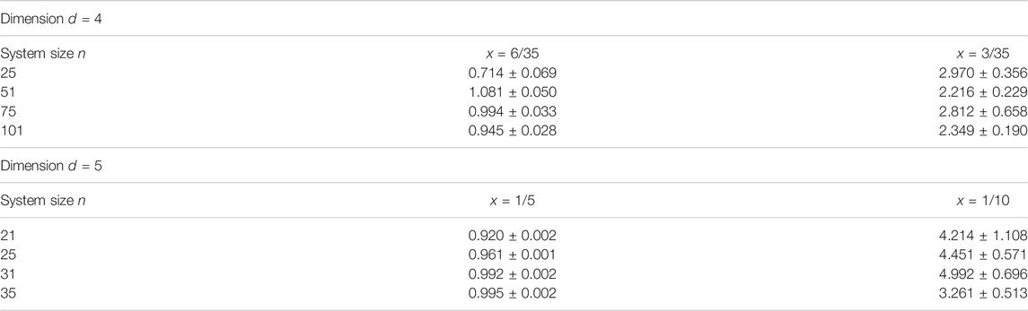
TABLE 1. The ratio of integrated autocorrelation times of the three-move nonreversible Berretti-Sokal algorithm, τ, and the two-move nonreversible Berretti-Sokal algorithm, τ₀, for 4D and 5D systems as a function of the linear system size n and the SAW unit step weight x. The ratio about 1 for (x = 6/35, d = 4) and (x = 1/5, d = 5), however for (x = 3/35, d = 4) and (x = 1/10, d = 5) it is above unity, which indicates that two-mode nonreversible Berretti-Sokal algorithm is more efficient there.

References

1. Hu H, Chen X, Deng Y. Irreversible Markov Chain Monte Carlo Algorithm for Self-Avoiding Walk. Front Phys (2016) 12:120503. doi:10.1007/s11467-016-0646-6

CrossRef Full Text | Google Scholar

2. Havlin S, Ben-Avraham D. New Approach to Self-Avoiding Walks as a Critical Phenomenon. J Phys A: Math Gen (1982) 15:L321–L328. doi:10.1088/0305-4470/15/6/013

CrossRef Full Text | Google Scholar

3. Havlin S, Ben-Avraham D. Theoretical and Numerical Study of Fractal Dimensionality in Self-Avoiding Walks. Phys Rev A (1982) 26:1728–34. doi:10.1103/physreva.26.1728

CrossRef Full Text | Google Scholar

4. Lawler GF, Schramm O, Werner W. On the Scaling Limit of Planar Self-Avoiding Walk. Fractal geometry Appl a jubilee Benoît Mandelbrot (2002) 2 339–64. doi:10.1090/pspum/072.2/2112127

CrossRef Full Text | Google Scholar

5. Flory P. Principles of Polymer Chemisty. Ithaca, NY: Cornell University Press (1953).

Google Scholar

6. Metropolis N, Ulam S. The Monte Carlo Method. J Am Stat Assoc (1949) 44:335–41. doi:10.1080/01621459.1949.10483310

CrossRef Full Text | Google Scholar

7. Janse van Rensburg EJ. Monte Carlo Methods for the Self-Avoiding Walk. J Phys A: Math Theor (2009) 42:323001. doi:10.1088/1751-8113/42/32/323001

CrossRef Full Text | Google Scholar

8. de Carvalho CA, Caracciolo S, Fröhlich J. Polymers and G|φ|4 Theory in Four Dimensions. Nucl Phys B (1983) 215:209–48. doi:10.1016/0550-3213(83)90213-4

CrossRef Full Text | Google Scholar

9. Duplantier B. Polymer Network of Fixed Topology: Renormalization, Exact Critical Exponentγin Two Dimensions, Andd=4−ε. Phys Rev Lett (1986) 57:941–4. doi:10.1103/physrevlett.57.941

PubMed Abstract | CrossRef Full Text | Google Scholar

10. Zhou Z, Grimm J, Fang S, Deng Y, Garoni TM. Random-Length Random Walks and Finite-Size Scaling in High Dimensions. Phys Rev Lett (2018) 121:185701. doi:10.1103/physrevlett.121.185701

PubMed Abstract | CrossRef Full Text | Google Scholar

11. Zhou Z, Grimm J, Deng Y, Garoni TM. Random-length Random Walks and Finite-Size Scaling on High-Dimensional Hypercubic Lattices I: Periodic Boundary Conditions. arxiv (2020).

Google Scholar

12. Fang S, Deng Y, Zhou Z. Logarithmic Finite-Size Scaling of the Self-Avoiding Walk at Four Dimensions. Phys Rev E (2021) 104:064108. doi:10.1103/PhysRevE.104.064108

CrossRef Full Text | Google Scholar

13. Sokal A. Monte Carlo Methods in Statistical Mechanics: Foundations and New Algorithms. In: C DeWitt-Morette, P Cartier, and A Folacci, editors. Functional Integration, Vol. 361 of NATO ASI Series, 131–192. New York, NY, USA: Springer US (1997). doi:10.1007/978-1-4899-0319-8_6

CrossRef Full Text | Google Scholar

14. Newman MEJ, Barkema GT. Monte Carlo Methods in Statistical Mechanics. Walton St. Oxford: Clarendon Press (1999).

Google Scholar

15. Madras N, Sokal AD. The Pivot Algorithm: A Highly Efficient Monte Carlo Method for the Self-Avoiding Walk. J Stat Phys (1988) 50:109–86. doi:10.1007/bf01022990

CrossRef Full Text | Google Scholar

16. Berretti A, Sokal AD. New Monte Carlo Method for the Self-Avoiding Walk. J Stat Phys (1985) 40:483–531. doi:10.1007/bf01017183

CrossRef Full Text | Google Scholar

17. Rensburg EJJv., Whittington SG. The BFACF Algorithm and Knotted Polygons. J Phys A: Math Gen (1991) 24:5553–67. doi:10.1088/0305-4470/24/23/021

CrossRef Full Text | Google Scholar

18. Diaconis P, Holmes S, Neal RM. Analysis of a Non-reversible Markov Chain Sampler (1997) Cornell University. Technical Report BU-1385-M.

Google Scholar

19. Chen F, Lovasz L, Pak I. Lifting Markov Chains to Speed up Mixing. In: Proceedings of the ACM symposium on Theory of Computing; 1999 May 1-4; New York, NY, United States (1999). p. 275–81. doi:10.1145/301250.301315

CrossRef Full Text | Google Scholar

20. Turitsyn KS, Chertkov M, Vucelja M. Irreversible Monte Carlo Algorithms for Efficient Sampling. Physica D: Nonlinear Phenomena (2011) 240:410–4. doi:10.1016/j.physd.2010.10.003

CrossRef Full Text | Google Scholar

21. Vucelja M. Lifting-A Nonreversible Markov Chain Monte Carlo Algorithm. Am J Phys (2016) 84:958–68. doi:10.1119/1.4961596

CrossRef Full Text | Google Scholar

22. Sakai Y, Hukushima K. Dynamics of One-Dimensional Ising Model without Detailed Balance Condition. J Phys Soc Jpn (2013) 82:064003. doi:10.7566/jpsj.82.064003

CrossRef Full Text | Google Scholar

23. Bierkens J, Roberts G. A Piecewise Deterministic Scaling Limit of Lifted Metropolis–Hastings in the Curie–Weiss Model. Ann Appl Probab (2017) 27:846–82. doi:10.1214/16-aap1217

CrossRef Full Text | Google Scholar

24. Bierkens J. Non-reversible Metropolis-Hastings. Stat Comput (2016) 26:1213–28. doi:10.1007/s11222-015-9598-x

CrossRef Full Text | Google Scholar

25. Kapfer SC, Krauth W. Irreversible Local Markov Chains with Rapid Convergence towards Equilibrium. Phys Rev Lett (2017) 119:240603. doi:10.1103/physrevlett.119.240603

PubMed Abstract | CrossRef Full Text | Google Scholar

26. Janse van Rensburg EJ, Rechnitzer A. Atmospheres of Polygons and Knotted Polygons. J Phys A: Math Theor (2008) 41:105002. doi:10.1088/1751-8113/41/10/105002

CrossRef Full Text | Google Scholar

27. Rechnitzer A, Rensburg EJJV. Canonical Monte Carlo Determination of the Connective Constant of Self-Avoiding Walks. J Phys A: Math Gen (2002) 35:L605–L612. doi:10.1088/0305-4470/35/42/103

CrossRef Full Text | Google Scholar

28. Rechnitzer A, Janse van Rensburg EJ. Generalized Atmospheric Rosenbluth Methods (GARM). J Phys A: Math Theor (2008) 41:442002. doi:10.1088/1751-8113/41/44/442002

CrossRef Full Text | Google Scholar

29. van Rensburg EJJ, Rechnitzer A. Generalized Atmospheric Sampling of Self-Avoiding Walks. J Phys A: Math Theor (2009) 42:335001. doi:10.1088/1751-8113/42/33/335001

CrossRef Full Text | Google Scholar

30. Levin DA, Peres Y, Wilmer EL. Markov Chains and Mixing Times. Providence, RI, USA: American Mathematical Society (2009).

Google Scholar

31. Metropolis N, Rosenbluth AW, Rosenbluth MN, Teller AH, Teller E. Equation of State Calculations by Fast Computing Machines. J Chem Phys (1953) 21:1087–92. doi:10.1063/1.1699114

CrossRef Full Text | Google Scholar

32. Hastings WK. Monte Carlo Sampling Methods Using Markov Chains and Their Applications. Biometrika (1970) 57:97–109. doi:10.1093/biomet/57.1.97

CrossRef Full Text | Google Scholar

33. Goodman J, Weare J. Ensemble Samplers with Affine Invariance. CAMCoS (2010) 5:65–80. doi:10.2140/camcos.2010.5.65

CrossRef Full Text | Google Scholar

34. Hsu H-P, Grassberger P. Polymers Confined between Two Parallel Plane walls. J Chem Phys (2004) 120:2034–41. doi:10.1063/1.1636454

CrossRef Full Text | Google Scholar

35. Owczarek AL, Prellberg T. Scaling of Self-Avoiding Walks in High Dimensions. J Phys A: Math Gen (2001) 34:5773–80. doi:10.1088/0305-4470/34/29/303

CrossRef Full Text | Google Scholar

36. Campbell S, Janse van Rensburg EJ. Parallel PERM. J Phys A: Math Theor (2020) 53:265005. doi:10.1088/1751-8121/ab8ff7

CrossRef Full Text | Google Scholar

37.I Guyon, UV Luxburg, S Bengio, H Wallach, R Fergus, S Vishwanathanet al. editors. A-NICE-MC: Adversarial Training for MCMC. Red Hook, New York: Curran Associates, Inc. (2017).

Google Scholar