 Lucia Carichino
 Derek Drumm2
 Sarah D. Olson
94% of researchers rate our articles as excellent or good
Learn more about the work of our research integrity team to safeguard the quality of each article we publish.
Find out more
ORIGINAL RESEARCH article
Front. Phys. , 01 November 2021
Sec. Social Physics
Volume 9 - 2021 | https://doi.org/10.3389/fphy.2021.735438
This article is part of the Research Topic Physics of Social Interactions View all 12 articles
Although hydrodynamic interactions and cooperative swimming of mammalian sperm are observed, the key factors that lead to attraction or repulsion in different confined geometries are not well understood. In this study, we simulate the 3-dimensional fluid-structure interaction of pairs of swimmers utilizing the Method of Regularized Stokeslets, accounting for a nearby wall via a regularized image system. To investigate emergent trajectories of swimmers, we look at different preferred beat forms, planar or quasi-planar (helical with unequal radii). We also explored different initializations of swimmers in either the same plane (co-planar) or with centerlines in parallel planes. In free space, swimmers with quasi-planar beat forms and those with planar beat forms that are co-planar exhibit stable attraction. The swimmers reach a maintained minimum distance apart that is smaller than their initial distance apart. In contrast, for swimmers initialized in parallel beat planes with a planar beat form, we observe alternating periods of attraction and repulsion. When the pairs of swimmers are perpendicular to a nearby wall, for all cases considered, they approach the wall and reach a constant distance between swimmers. Interestingly, we observe sperm rolling in the case of swimmers with preferred planar beat forms that are initialized in parallel beat planes and near a wall.
The tumultuous journey of the mammalian sperm involves navigating the female reproductive tract. Even though millions of sperm are deposited at the beginning of the tract, only a select few are able to traverse the long distances and overcome all of the hurdles to make it to the egg [1, 2]. Using a single flagellum, sperm progress through a wide range of environments and their motility patterns must change in response to various chemical and physical cues; this could act to group sperm together or separate them [3–5]. A sperm senses other nearby sperm and surfaces via hydrodynamic interactions, which results in a wide range of collective motion, from alignment in trains and vortices to synchronization and attraction [6–8].
Sperm are able to propel themselves through different fluid environments by bending their elastic and flexible flagellum or tail. Within the flagellum, dynein is the molecular motor that actively generates force along the length of the flagellum, which results in a bending wave [2, 9–11]. The emergent beat form and trajectory will depend on the local fluid environment and the particular species of sperm. In experiments, emergent planar, helical, and quasi-planar flagellar beat forms have been observed, with planar beat forms more likely in higher viscosity fluids [10, 11]. Similarly, tracking of sperm trajectories has shown linear trajectories as well as helical trajectories [12, 13].
Surface interactions play an important role of many micro-organisms, including sperm swimming in the reproductive tract [6, 14]. Once sperm reach the oviduct, they generally bind to the epithelial cell wall and remain in this sperm reservoir until the time of ovulation [15]. At ovulation, signaling molecules such as heparin or progesterone will increase in concentration and will aid in the release of the sperm from the oviductal wall [15–17]. Likely, these signaling molecules will either act to break bonds of the cell body with the wall or bind to the flagellum and initiate a different beat form that will aid in generating increased force to break away from the wall [18, 19]. There are many interesting and unanswered questions as to how sperm get to the walls, how long they stay at the walls, as well as how the sperm reservoir could act as a filter to sort out healthy sperm [20, 21]. Investigations with microfluidic channels have revealed that sperm guidance can be achieved with surface topography and microchannels [22, 23].
There are many different modeling approaches that can be taken to model sperm motility, but one of the key ingredients is how the sperm cell itself is being represented. Simplified approaches neglect the head or cell body [24–26]; headless sperm can still swim and previous analysis has shown that neglecting the cell body results in similar dynamics [27, 28]. Other studies have focused on capturing accurate cell body geometries to investigate the role on swimming and interactions [29–31]. Similarly, when accounting for the bending of the flagellum, there are a few options. One can actuate or drive the dynamics of the flagellum with forces or torques corresponding to a curvature wave [24, 32], prescribe a preferred curvature that is utilized in an energy functional that determines forces [25, 26, 33], or exactly prescribe the beat form [29–31]. When the beat form is prescribed exactly, the swimmer may rotate, but the flagellum will always have its entire centerline in the same plane and it will always have the same beat form parameters (e.g., amplitude and beat frequency). Preferred beat forms will have emergent beat forms based on interactions with other swimmers and/or surfaces.
To date, there have been many studies that have investigated the 3-dimensional (3D) dynamics of a single sperm near a wall [10, 19, 34]. Wall attraction was observed when approaching at specific angles, including perpendicular to the wall. Similarly, there have been studies of pairs of swimmers in free space to study the dynamics of attraction since biologically, most sperm are not swimming in isolation [24–26, 31]. Since there has not been a detailed study of the interactions of pairs of swimmers near a wall, our goal is to further investigate and characterize how pairwise interactions vary from free space to the case where the sperm are swimming in close proximity and perpendicular to a planar wall. Using the method of regularized Stokeslets with an image system to account for the wall, we study swimmers propagating both preferred planar and quasi-planar beat forms. The dynamics of attraction and repulsion of swimmers is explored through different configurations; we vary both the initial distance between the sperm as well as the planes in which the swimmers are initialized. Our results show that sperm will attract to and stay near the wall while phenomenon such as sperm rolling will occur for a subset of sperm configurations. Our results further contextualize divergent results for pairs of swimmers in previous studies and provides insight into relevant interactions that can be utilized in the development of artificial micro-swimmers [35–37].
We utilize a fluid-structure interaction framework where the sperm is assumed to be neutrally buoyant and immersed in the fluid. Since sperm swim in viscosity dominated environments and are often in close proximity to a wall or boundary [2, 38], we will consider the 3-dimensional (3D) incompressible Stokes equations for the fluid velocity u above a planar wall at
subject to the boundary condition
To determine the body forces, we will study a simplified representation of a sperm cell where we neglect the cell body, similar to previous studies of [32, 39]. Additionally, we assume the sperm flagellum is isotropic and homogeneous with constant radius much smaller than length L so that we can represent it using the Kirchhoff Rod (KR) model. This allows for each cylindrical elastic flagellum ι to be represented via a space curve Xι(t, q) for arc length parameter q (0 ≤ q ≤ L). Local twisting is accounted for via a right-handed orthonormal triad,
In the KR model, through a variational energy argument, we can define the internal force Fι and torque Mι on a cross section of flagellum ι as
where δ3i is the Kronecker delta and
Sperm propagate bending along the length of the flagellum due to the coordinated action of molecular motors inside the flagellum [2, 47]. We can capture a range of beat forms representative of experimental observations [9, 10] by assuming that the flagella have the preferred configuration of
with beat frequency f = ω/2π, wavelength 2π/η, and beat amplitudes α and β. Planar bending of the flagellum occurs when either α or β are zero whereas quasi-planar bending occurs when α, β ≠ 0 and either α < β or β < α. We note that we are not prescribing a rotation of the flagellum; we simply actuate or drive it to beat (and bend) in this preferred planar or quasi-planar configuration that is a function of arc length parameter q and time t. Similarly, these are the initialized and preferred configurations that can deviate later in the simulation due to interactions with other swimmers and/or the wall. Utilizing this preferred configuration, we can calculate the preferred orthonormal triad
which is a spatiotemporal function based on
For this configuration, we impose force and torque balance along the length of the flagellum. That is, the fluid feels the sperm through a force per unit length fι and torque per unit length mι [only defined on Xι(q, t)],
The body force
where Γι = Xι(q, t), x is any point in the 3D domain with
where
We discretize each of the
where
which ensures that the boundary condition at the wall is satisfied,
To solve this coupled fluid-structure interaction, at each time point t, we complete the above steps to determine the resulting linear and angular velocity due to a given flagellar configuration (assuming the preferred configuration in Eqs 3, 4). Once the velocity of the flagellum, u (Xι), and angular velocity of the triads, w (Dι), are known, we determine the new flagellar location and triads at time t + τ by solving the no-slip equations in Eq. 7 with the forward Euler method. This process is repeated, solving for the new instantaneous flow due to each time-dependent force balance equation, which depends on the emergent flagellar configurations. We emphasize that this is a Lagrangian method; only the flagella are discretized. Through the regularized image system in Eq. 8, we automatically satisfy that the wall at
The actual beat form, swimming speed, and trajectory that the sperm achieves is an emergent property of the coupled system that depends on both the geometry of the swimmers and the wall, fluid parameters such as viscosity, beat form parameters, as well as stiffness or moduli of the flagella. We will explore these dynamic and nonlinear relations through simulations. Here we highlight some of the metrics and different parameters that are studied.
The sperm number is a non-dimensional number that characterizes the ratio of viscous fluid effects to elastic effects of the bending flagellum, computed as
Here, L is the flagellum length, f is the beat frequency (inverse time), ɛ is the regularization parameter that approximates the flagellum radius, μ is fluid viscosity, and a1 is the bending modulus. To compare to previous studies, we utilize the resistive force theory coefficient χ to capture viscous effects, similar to [32]. For mammalian sperm, previous estimates have had Sp in the range of 2–17 [2]. Using the values reported in Table 1, the baseline sperm number for our simulations is Sp = 5.11. We explore increasing Sp to a value of 7.64 by increasing μ to 5μ and increasing Sp to 9.08 by increasing μ to 10μ. Similarly, we also explore increasing Sp by setting ai to ai/5 or ai/10 for i = 1, 2, 3. Even though this leads to the same sperm number, we explore the differences since a change in μ changes the magnitude of all terms in Eq. 8 whereas a change in ai only changes the magnitude of the terms involving the torque, which can be seen from Eq. 2.
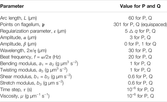
TABLE 1. Computational parameters for preferred planar (P) and quasi-planar (Q) beat forms.
Through interactions, the beating planes of swimmers may continue to deviate from the plane they were initialized in. A diagram of the directions of pitching and/or rolling out of the beating plane is given in Figure 1. The beating plane is calculated as the plane that passes through the center of mass
where n is the normal vector to the beating plane. The pitching angle θ is in the range [ −90°, 90°] and θ > 0 (θ < 0) corresponds to the plane pitching upward (downward). The rolling angle γ of the swimmer’s beating plane is the angle between the plane and the unitary vector in the y-direction ey,
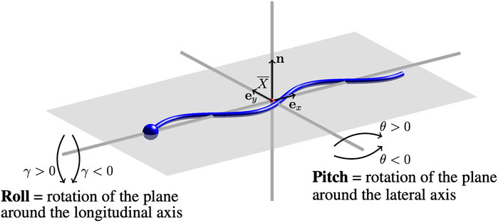
FIGURE 1. Pitching and Rolling of Flagellar Beating Planes. A sketch of the swimmer (blue) and the beating plane (gray). Changes in the initial beating plane are characterized by a pitching angle θ and rolling angle γ. The center of mass of the swimmer
The rolling angle γ is also in the range [ −90°, 90°] and γ > 0 (γ < 0) corresponds to the plane rolling right (left) with respect to the direction of motion.
The aim of this study is to further quantify and understand the hydrodynamic interactions of pairs of swimmers close to or far away from a wall. To do this, we will consider a few different scenarios that include planar or quasi-planar beat forms initialized a distance d apart. For the case of planar beat forms, we also consider the case of flagellar beating with centerlines initialized in parallel planes or the same plane (co-planar). The wall is either initialized at x = −5 (near a wall) or at x = −10,000, which we denote as the free space solution since the wall has negligible effects on swimming at this location. The baseline parameters used for the numerical methods and preferred beat form are given in Table 1; we assume that in a given simulation, all sperm flagella have the same preferred configuration given by Eqs 3, 4, with values in the range of mammalian sperm [10]. Swimmers are separated by a distance d in either the y or z-directions. We explore distances d in the range of 3–30 μm, i.e., distances where there is non-negligible flow effects from the nearby swimmer. Here, 30 μm is half the length of the swimmer (L = 60 μm) and 3 μm is equal to the beat amplitude α.
This case involves two planar swimmers (α = 3 and β = 0 in Eq. 3) initialized such that their initial beating planes are in the plane z = 0, shifted a distance d apart in the y-direction. That is, the average y-value,
Figure 2A shows the configuration of two co-planar sperm cells at time t = 0 (gray dashed lines) and at time t = 0.6 s (gray solid lines) for swimmers initialized d = 6 μm apart. The first point is represented by a solid gray circle and denotes the cell body and swimming direction. The trajectories of the first point during this time frame (blue and black solid lines) show the hydrodynamic attraction of the two sperm cells; the top sperm starts to go down and attract to the bottom sperm, which is swimming with an upward trajectory. We classify this movement as yaw since these motions remain within the plane z = 0, which has been observed in other modeling work for a single swimmer [29, 30, 34]. A solo swimmer has an upward yaw [34], but attraction dominates and allows the top swimmer to have a downward yaw and attract to the bottom swimmer. This attraction is also in agreement with previously published theoretical and experimental studies [24–26, 31, 33, 53].
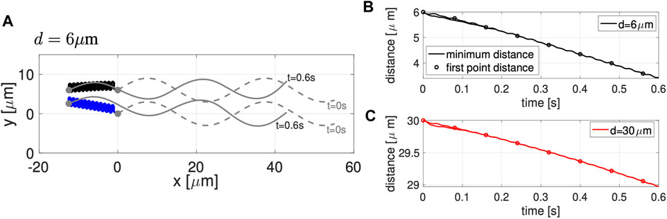
FIGURE 2. Co-Planar Sperm in Free Space. (A) Swimmer configurations with planar preferred beat forms at t = 0 s (dashed gray lines) and t = 0.6 s (solid gray lines), and traces of the first point on the swimmer in time (blue and black solid lines) for the initial separation distance of d = 6 μm. Minimum distance between the two sperm (solid lines) and distance between the first points of the two swimmers (circles) in time, for initial distances d = 6 μm (B) and d = 30 μm (C). Distances reported are the average over a beat period.
Figures 2B,C track the minimum distance between the two sperm (solid lines) and the distance between the first points of the two sperm (circles) as a function of time, for the initial distances d considered. In both cases, for d = 6 and d = 30 μm, we observe a monotonic decrease in the distance between the sperm for this initial time period of attraction, similar to results of [26]. Even though the sperm are initialized at the same distance d apart along the entire flagellum, the minimum distance between the sperm cells occurs at the head (first point). For longer time simulations, we continue to observe attraction, reaching a steady configuration of flagella that are a very small distance apart. We do not show simulations or report this distance since a repulsion term is required to keep the filaments from occupying the same space and hence, the steady state distance between the flagella will depend on the strength and form of the repulsion term.
We also varied the sperm number Sp (given in Eq. 10); similar dynamics of attraction were observed but on a slower time scale (results not shown). As previously noted in [32], for a solo swimmer, increasing Sp results in a decreased swimming speed. We observe a similar decrease for a pair of swimmers with increased Sp, which leads to the increased time scale for attraction to occur.
Previous studies with planar beat forms required to stay in the plane have reported an increase in swimming speeds for pairs of swimmers relative to the case of a solo swimmer when filaments propagate planar beat forms, are co-planar, and the flagella are sufficiently stiff [25]. Other studies that allow beat forms to deviate from the plane have reported a slowdown of swimming speed while swimmers attract [26]. For the parameters utilized in Figure 2 (reported in Table 1), we observe a decrease in swimming speed for a pair of swimmers initialized d = 6 μm apart and a small increase in swimming speed for a pair of swimmers initialized d = 30 μm. The speeds reported in Table 2 are looking at the magnitude of velocity of the first point on the flagellum by utilizing locations at time t = 0 and t = 0.6 s; for two swimmers, the speed is the average over both swimmers. We do not observe a significant increase in swimming speed during the attraction phase for a range of initial separation distances. However, on longer time intervals after attraction has occurred, we do observe an increase in swimming speed (results not shown).
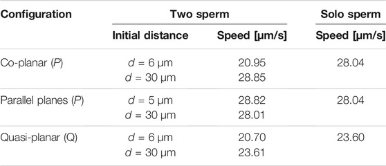
TABLE 2. Swimming speeds in free-space for the preferred planar (P) beatform in co-planar or parallel beating planes and quasi-planar (Q) beat forms, comparing the two sperm configuration initialized d apart to the solo sperm.
We have shown that our model can capture a range of known phenomena for a pair of swimmers in free space, but sperm are not swimming in isolation and they are swimming in close proximity to walls as they navigate the female reproductive tract [2, 5]. Hence, we wish to go beyond previous studies of a pair of swimmers in free space or a solo swimmer near a wall to understand whether the wall will help or hinder attraction of swimmers. For a solo swimmer, simulations have shown attraction to a wall is immediate but no yawing motion or vertical translation (up or down with respect to the centerline of the flagellum) is observed [34]. We note that for a solo swimmer initialized perpendicular to the wall, it will always attract to the wall regardless of whether it starts 2 μm or 50 μm away (the wall does not cause the swimmer to tilt and escape the wall). The questions are now 1) will additional sperm change the dynamics of attraction to a wall; 2) will swimmers near a wall still be able to attract to each other; 3) if attraction occurs, will it happen with heads decreasing their distance apart at a faster rate (similar to Figures 2B,C)?
To study these questions, we consider the case of two co-planar swimmers initialized at a distance d apart and perpendicular to a planar wall at x = −5 μm. Figure 3 shows the configurations of the swimmers at time t = 0 (gray dashed lines) and at three snapshots in time (gray solid lines), for the initial distance of d = 3 μm in A, d = 6 μm in B, and d = 11 μm in C. The first point of the swimmer is represented by a solid gray circle and the trace of this point (from t = 0 until the time point given in that panel) is shown with the solid lines. For all values of d considered, the swimmers start with the head 5 μm away from the wall and rapidly attract to the wall, remaining close to the wall for the full time of the simulation (over 2.5 s).
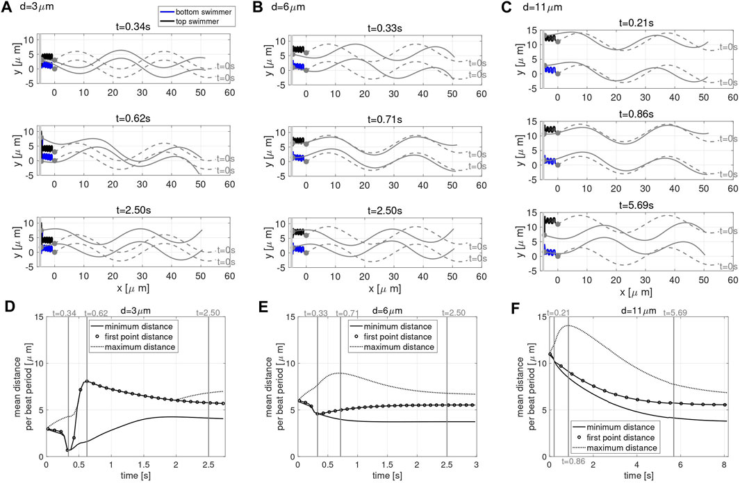
FIGURE 3. Co-Planar Sperm Near a Wall. Swimmer configurations with planar preferred beat forms at t = 0 s (dashed gray lines) and at three snapshots in time (solid gray lines) for the initial distance d = 3 μm (A), d = 6 μm (B) and d = 11 μm (C) with a planar wall at x = −5 μm. The traces of the first point on the swimmer are shown (blue and black solid lines). The time-dependent distance between swimmers is characterized in (D)–(F). For initial swimmer distances of d = 3 μm (D), d = 6 μm (E) and d = 11 μm (F), the minimum (solid line), maximum (dashed line), and first point distance (circles) are reported as averages over each beat period. The times chosen to report the swimmer configurations for each value of d (A–C) are identified with vertical gray lines in the corresponding distance graphs (D–F). The thick gray vertical line in (A–C) represents the wall.
In order to explore the rich dynamics of swimmers near a wall, we also report the minimum (solid line) and maximum (dotted line) distance between the two swimmers, along with the average distance between the first points of the two swimmers (circles) in Figure 3, for initial distance d = 3 μm in D, d = 6 μm in E and d = 11 μm in F. The snapshots in time in A–C are identified with vertical gray lines in the corresponding distance graphs in D–F, and were chosen to highlight specific points of interest. The top panel in Figures 3A–C is the last time point for which the distance between the first points equals the minimum distance between the swimmers, i.e., the end of the first attraction period between the two swimmers where the heads are moving closer. The middle panel in Figures 3A–C is where the maximum distance between the swimmers is at a maximum. The stable configuration achieved by the swimmers is shown in the bottom panel in Figures 3A–C. Here, we are defining stable as attaining an average distance between points on the swimmer that persists in time. The same preferred beat form is given for all swimmers in all of these simulations; the presence of the wall and the initial separation distance is what causes the different beat forms to emerge. We note that two swimmers in free space attract, with the top swimmer yawing down and the bottom swimmer yawing up (Figure 2B). The dynamics of the nearby wall prevent the swimmers to attract with equal yawing due to the emergent flagellar beat forms.
For all the values of d considered, the stable configuration achieved toward the end of the simulation (third snapshot) consists of an average first point distance of approximately 5.5 μm, in between the maximum and minimum average distance between the swimmers. As shown in Figures 3A,D, for an initial distance d smaller than 6 μm, the swimmer’s first points initially attract, reaching a minimum distance on the order of 1 μm at t = 0.34 s, then repulse reaching the maximum average distance of approximately 8 μm at t = 0.62 s (with the top swimmer moving up). Due to hydrodynamic interactions of the swimmer and the close wall, even though the swimmers have centerlines that are parallel, we observe a dramatic yaw in the top swimmer as the head of the top swimmer is pushed up. Later, the swimmers reach a stable configuration after 2.50 s where flagellar centerlines are again parallel. For an initial distance d equal to 6 μm, shown in Figures 3B,E, the head of the swimmers (first point) attract up until t = 0.33 s, reaching a distance of approximately 4.5 μm. After this initial attraction, the heads of the swimmer then repulse, reaching a maximum distance 9 μm apart at t = 0.71 s, and reach the stable configuration after 2.50 s. For an initial distance d greater than 6 μm, Figures 3C,F, the maximum distance of 14 μm between the swimmers is reached at t = 0.86 s and the distance between the first points show a continuous decrease in time until reaching a plateau and the stable configuration after 5.69 s. In this last scenario, the top swimmer, after reaching the wall, is moving downward to get closer to the bottom swimmer, clearly visible in Figure 3C at t = 5.69 s. The asymmetry between the swimmer’s behavior is due to the direction of motion chosen. When the direction of motion is reversed (wall at x = 5, swimmers reflected about the y-axis, and preferred beat form propagating a wave in the opposite direction with − ω), we observe the bottom swimmer moving upward to get closer to the top swimmer (results not shown).
To explore competing effects of wall attraction and swimmer dynamics, we vary the sperm number Sp in Eq. 10. Figure 4 shows the swimmer configurations obtained for the different values of Sp considered in the case of two co-planar swimmers near a wall, varying μ in A,B,E and varying ai in C,D,F. Increasing Sp means that the viscous effects are increasing relative to the elastic effect. As a result, in both Figures 4A–D, increasing Sp exhibits a beat form with decreased achieved amplitude. In A,B, this is due to the increased viscosity of the fluid creating additional drag on the bending flagellum whereas in C,D, this is due to the decrease in the bending moduli making the flagellum less stiff and less able to propagate bending at the preferred amplitude. Even though the achieved amplitude of the flagellar beat form decreases, this does not prevent or slow down attraction to the wall (shown in zoomed views in B and D). Through a close examination of the distance between the swimmers at different time points, we can see the subtle differences between increasing Sp via increasing μ in Figure 4E and decreasing ai in Figure 4F. The baseline value of Sp = 5.11 exhibits attraction and then repulsion with the heads being further apart than the rest of the flagellum at later time points (Figures 4E,F) and reaching a steady state configuration by t = 2 s. In contrast, if an increase in Sp to 7.64 or 9.08 is obtained by increasing μ by a factor 5 or 10, the swimmers do not maintain a stable configuration near the wall, but they continue to attract with the heads being the closest points at later time points (Figure 4E). Increased Sp in Figure 4E results in continued attraction whereas increased Sp in Figure 4F results in a quasi steady state configuration at t = 2 s.
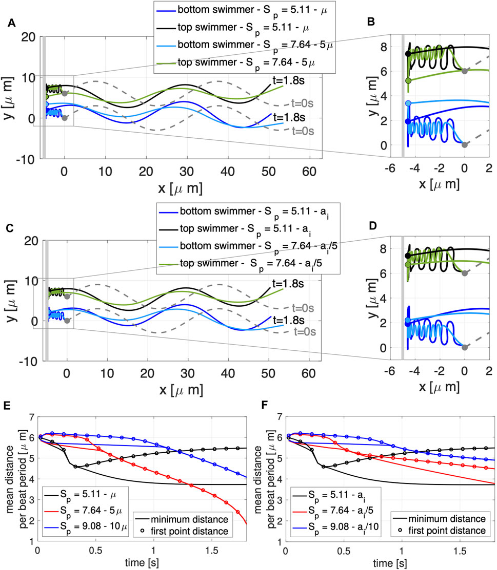
FIGURE 4. Varying Sperm Number: Co-Planar Sperm Near a Wall. Swimmers with planar preferred beat forms are initialized a distance d = 6 μm apart with a planar wall at x = −5 μm. Configurations at t = 0 s (gray dashed lines) and t = 1.8 s (colored solid lines) are shown along with traces of the first point on the flagellum for varying fluid viscosity in (A), with zoomed in view in (B), and varying flagellar material parameters ai in (C), with zoomed in view in (D). The thick gray vertical line in (A)–(D) represents the wall. The minimum distance between the two swimmers (solid lines) and distance between the first points of the two swimmers (circles) are shown as averages over a beat period, varying μ in (E) and ai in (F).
We emphasize that for all simulations presented here for co-planar swimmers near a wall, the swimmers had a preferred planar configuration. With swimmer interactions and the presence of the wall, there was some out of plane motion, but on average, the swimmers tended to maintain a beat form in the same plane (due to torques in Eq. 2 that penalize deviations from the preferred motion). Additionally, for all simulations, the head or first point of the swimmers attract to the wall and maintains a small distance away from the wall. This occurs for a range of parameters in the case of two swimmers and also occurs on a similar time scale to that of a solo swimmer [34]. For a sperm number of Sp = 5.11, in the range for mammalian sperm, we observe swimmers reaching a somewhat steady state distance of ∼5.5 μm within a few seconds when starting in the same plane at a distance of 3–11 μm apart. Since the beat frequency of the swimmers is set to f = 20 Hz; attraction on the order of seconds near the wall requires hundreds of beats of the flagellum. The dynamics of attraction will depend on the sperm number and increased Sp (increased viscous forces) results in sperm being able to attract closer at the first point or cell body. This is important to consider since the epithelial cells on the oviductal walls may be secreting proteins and/or fluids that will change the viscosity near the walls [54] and potentially control or dominate emergent interactions and motility of sperm [55].
It is well known that as mammalian sperm navigate through the female reproductive tract, their motility patterns change in response to different signaling molecules, which may be released from the wall or be present in the entire fluid [2, 3, 5]. When sperm are trapped on the oviductal walls, signaling molecules such as heparin or progesterone initiate changes in motility by binding to the cell body or the flagellum [15, 16]. In turn, changes to asymmetrical beating occur, which aids in the release of these trapped sperm [15–17, 19]. The ability for these molecules to reach the sperm and bind to receptors is highly dependent on the local fluid flows. In Figure 5, we look at the mixing of the fluid by the swimmers in the case of an initial separation of d = 3 μm in A,B and a separation of d = 11 μm in C,D. The left hand side (A,C) is the case of the wall at
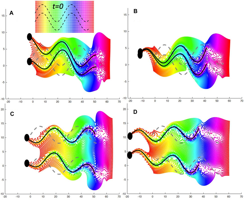
FIGURE 5. Fluid Mixing by Co-Planar Swimmers. A plane of fluid markers was initialized at t = 0 with x ∈ [0, 60] and either y ∈ [ −4, 7] when d = 3 μm or y ∈ [ −4, 16] when d = 11 μm, as shown on the inset in (A); fluid markers are colored by initial x-value. The fluid markers are advected by the flow and are shown at later time points with the same color as at t = 0. (A): d = 3 μm and a nearby wall at x = −5 at t = 0.882 s, (B): d = 3 μm and free space at t = 0.804 s, (C): d = 11 μm and a nearby wall at x = −5 at t = 0.882 s, (D): d = 11 μm and free space at t = 0.804 s. The gray dashed lines correspond to the initial location at t = 0 and the solid black lines correspond to the flagellar configurations at the specified time point.
We continue to consider the case of two planar swimmers (α = 3 and β = 0 in Eq. 3), but now these swimmers are initialized with parallel beating planes. The distance d between the swimmers is initialized by placing the bottom swimmer in the plane z = 0 and the top swimmer in the plane z = d. However, the emergent beat plane may pitch upward or downward in the z-direction and/or roll left or right around the lateral axis (refer to Figure 1 for a schematic). Similar to the co-planar case, we wish to first benchmark our model and further explore the case of swimmers far away (free space) or close to a wall to understand how these dynamics change.
The results in the case of free space are reported in Figure 6. The short-term simulations, up to t = 3.25 s, are shown in Figures 6A–D. A non-monotonic behavior depending on the initial distance d between the swimmer’s beating planes is observed. For d = 5 μm, the distance between the first points of the two swimmers increases in time (Figure 6A) while the rest of the swimmers slightly attract and then slowly increase their distance. The beating plane of the bottom swimmer pitches downward while the top swimmer pitches upward by angles of ±2.3° at t = 3 s (Figures 6B,C), corresponding to the swimmers pushing away from each other. In contrast, for d = 30 μm, the distance between the first points of the two swimmers decrease in time (Figure 6A), attracting with the beating plane of the bottom swimmer pitching upward and the top swimmer pitching downward with angles of ±1.6° (Figures 6B,D). In the shorter time simulations (Figures 6A–D), the beating plane of both swimmers have a minimal rolling motion, alternating between left and right rolling with −0.26° ≤ γ ≤ 0.26° for d = 5 μm and −0.14° ≤ γ ≤ 0.14° for d = 30 μm.
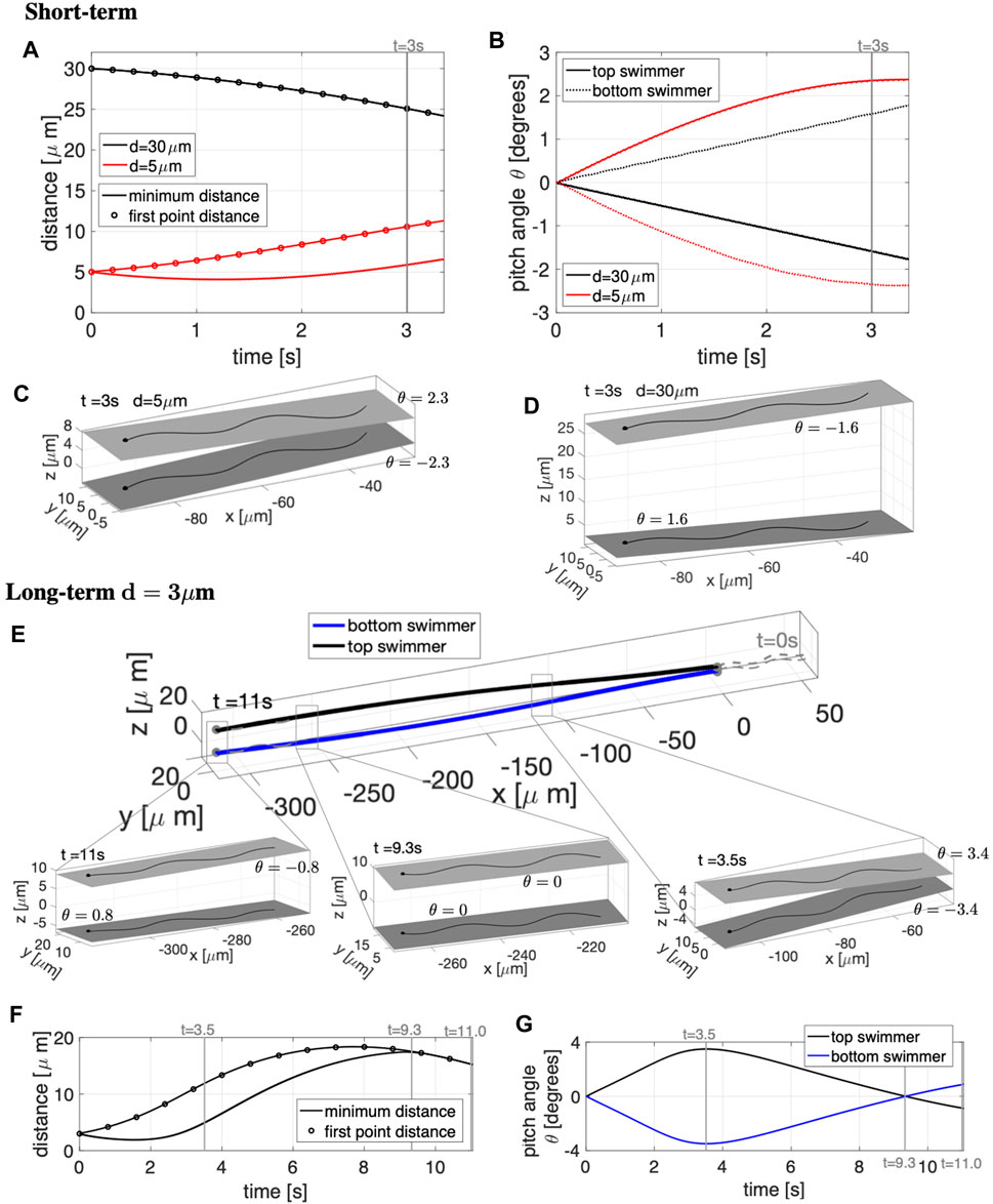
FIGURE 6. Parallel Sperm in Free Space. Short-term behavior for initial distances d = 5, 30 μm (A–D) and long-term behavior for d = 3 μm (E–G) for swimmers initialized in parallel beating planes. Minimum distance between the two swimmers (solid lines) and distance between the first points of the two swimmers (circles) in time, for initial distances d = 5, 30 μm in (A) and d = 3 μm in (F). Pitching angle θ of the beating planes of the top and bottom swimmers in time, for initial distances d = 5, 30 μm in (B) and d = 3 μm in (G). Top and bottom swimmer’s beating planes and pitching angles θ for d = 5 μm in (C) and d = 30 μm in (D) at time t = 3 s. (E) Swimmer configurations at t = 0 s (gray dashed lines) and traces of the swimmers initial points in time (colored solid lines). Top and bottom swimmer’s beating planes and pitching angles θ for three snapshots in time are reported in the corresponding zoomed portions. The times chosen for the zoomed portions of (E) are identified with vertical gray lines in (F,G). In (C,D,E), a filled in sphere is used to denote the swimmer first point in the direction of motion.
In terms of the swimming speeds for these shorter term dynamics over 3 s, the swimming speed of two parallel swimmers was similar to the corresponding solo swimmer (Table 2). This is similar to previous results for pairs of swimmers separated by a distance of at least half their length, swimming speeds are similar to that of a solo swimmer [24, 26, 31]. However, we observe marked differences between swimmers that are co-planar and those that are in parallel planes. At an initial separation distance of d = 6 μm, the swimmers in parallel planes are significantly faster (∼28 μm/s) than the case of the co-planar swimmers (∼20 μm/s).
To investigate the long-term dynamics, we look at an initial separation of d = 3 μm for t = 0–11 s in Figures 6E–G. The zoomed in portions of Figure 6E show the top and bottom swimmer’s beating planes and corresponding pitching angles θ for the three snapshots in time, delineating the switches among near-field, mid-field and far-field dynamics. The times of the snapshot are identified with vertical gray lines in Figures 6F,G. The swimmers show near-field repulsion until t = 3.5 s, i.e., with heads or first points increasing in separation (Figure 6F) and beating planes pitching away from each other (Figure 6G and right-most zoomed portion of Figure 6E). The top and bottom swimmer’s beating planes obtain their maximum pitching angle at t = 3.5 s and after t = 3.5 s, the swimmers enter the mid-field regime where they will continue to repel each other (Figure 6F) but the pitching angles will decrease in magnitude (Figure 6G) and reach θ ≃ 0 at t = 9.3 s (central zoomed portion of Figure 6E). After t = 9.3 s, the swimmers show far-field attraction, i.e., decreasing distance between the swimmers (Figure 6F) with beating planes pitching toward each other (Figure 6G and leftmost zoomed portion of Figure 6E). In the long-term simulations, the rolling of the beating planes is also minimal, with −0.38° ≤ γ ≤ 0.38° over 11 s.
In summary, swimmers that are close to each other will initially show near-field repulsion and then eventually, after reaching a significant distance between each other, will transition to far-field attraction (Figure 6E). Conversely, if the swimmers are initialized relatively far away from each other, the swimmers will initially show far-field attraction and then eventually, when getting too close to each other, will transition to near-field repulsion (results not shown for d = 14 μm). Hence, dynamics of swimmers with planar beat forms in initially parallel beating planes will not reach a stable configuration of attraction and will continue to oscillate between attraction and repulsion. Our far-field attraction results differ from previous results of [26] where only repulsion was observed and [31] where only attraction is observed; this is likely due to different modeling assumptions with regards to the preferred planar beat form, how out of plane beating is penalized, and geometry of the cell body. We note that rotations of swimmers with respect to θ and γ are also on par with previous studies [24].
Similar to the previous cases, we wish to understand whether pairs of swimmers initialized in parallel planes will attract or repulse when near a wall. Results for the case of a wall at x = −5 μm are highlighted in Figure 7. For all the values of d considered, the swimmers also attract to the wall (similar to the case of initially co-planar swimmers in Figures 3, 4). When the swimmers are initialized d = 3 μm apart, they push apart and then quickly reach a constant distance apart (Figure 7A) whereas in free space, they continued to push apart initially (Figure 6A) and then oscillate between attraction and repulsion in the long term (Figure 6E). With the wall, the beating plane of the bottom swimmer pitches downward while the top swimmer pitches upward, but at a very small angle (Figures 7B,C). For the full ∼ 4 s simulation, the beating planes show minimal rolling behavior with −0.91° ≤ γ ≤ 0.91°. For the case of an initial distance of d = 30 μm, we observe constant attraction in Figure 7A, similar to the free space case in Figure 6A. In Figure 7A, the average distance between the two swimmers decreases monotonically in time for t ≥ 2.5 s. To understand why the first point or head distance is in between the minimum and maximum distance, we can see in Figure 7D that the entire length of the flagellum is not remaining in the same plane. The beating plane of the bottom swimmer pitches upward while the top swimmer pitches downward (i.e., toward each other), with a more preeminent rolling motion of the swimmer’s beating planes (Figures 7B,D), with −3.29° ≤ γ ≤ 3.29° for d = 30 μm.
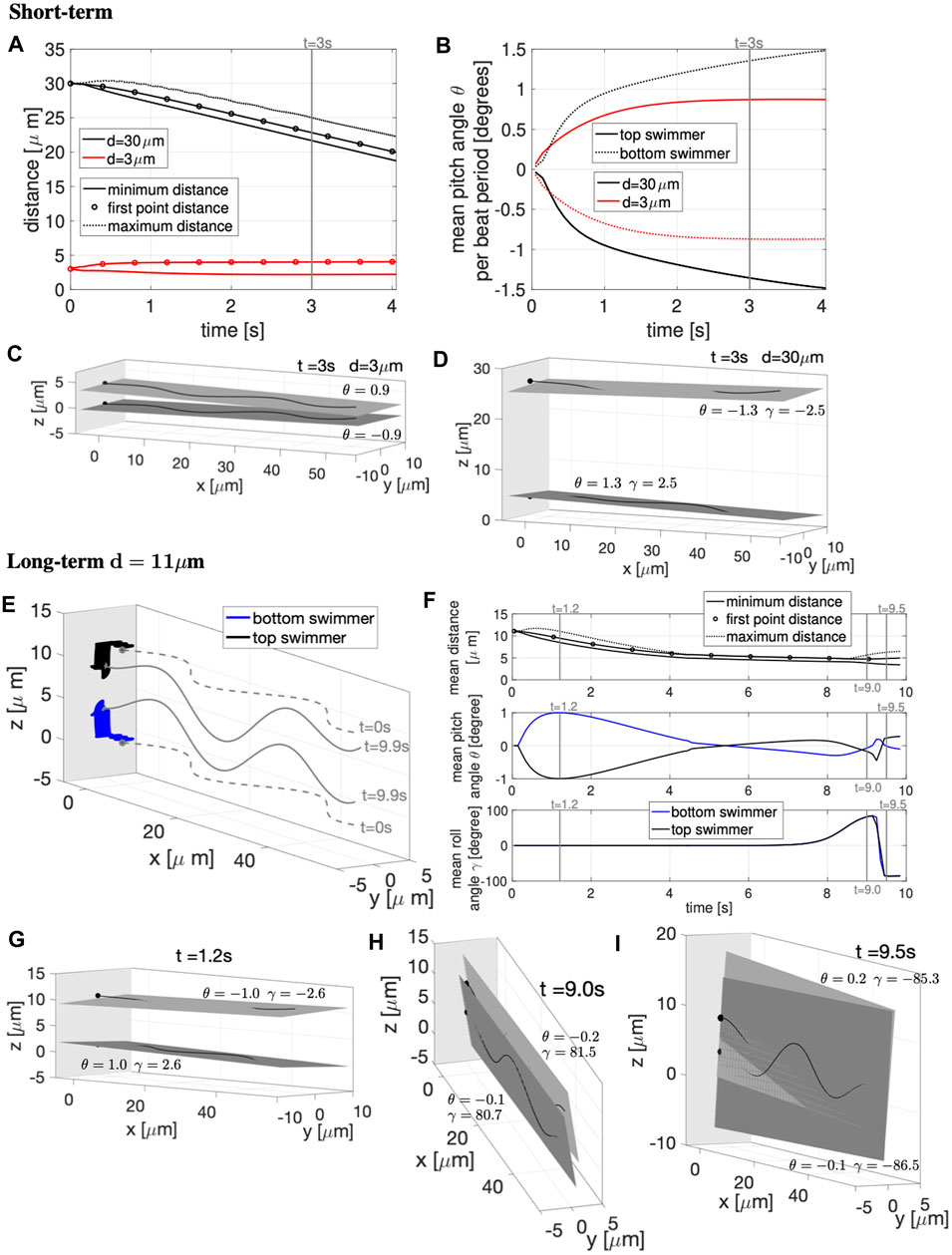
FIGURE 7. Parallel Sperm Near a Wall. Sperm with planar beat forms initialized in parallel planes (z = 0 and z = d) near a wall at x = −5 μm. (A–D): Short-term behavior for initial distances d = 3, 30 μm. (A) Minimum (solid lines) and maximum (dotted lines) distance between the two swimmers and distance between the first points of the two swimmers (circles). (B) Pitching angle θ of the top and bottom swimmers in time. The top and bottom swimmers beating planes for d = 3 μm is in (C) and d = 30 μm is in (D), both at time t = 3 s. (E–I): Long-term behavior for d = 11 μm. (E) Swimmer configurations at t = 0 s (gray dashed lines) and traces of the first point in time (colored solid lines). Corresponding beating planes of the swimmers for three snapshots are in (G–I). The times chosen for the snapshots are identified with vertical gray lines in (F), which has distance between the swimmers in the top panel, pitching angle θ in the middle panel, and rolling angle γ in the bottom panel. In (C–E,G–I), a filled in sphere is used to denote the swimmer first point in the direction of motion. The light gray plane in (C–E,G–I) represents the wall (and the darker gray planes are the beating planes).
To investigate the long-term behavior, we report in Figures 7E–I the results for d = 11 μm for ∼ 10 s. Figure 7E shows the swimmer configurations at t = 0 s (gray dashed lines) and traces of the first point or head in time (colored solid lines). Figures 7G–I shows the top and bottom swimmer’s beating planes and corresponding pitching and rolling angles (θ and γ) for three snapshots in time. The times coincide with the vertical gray lines in Figure 7F. When initialized at d = 11 μm, the swimmers show far-field attraction until t ≃ 4 s, reaching an average distance apart of ∼5 μm (Figure 7F top panel). The top and bottom swimmer’s beating planes obtain their maximum average pitching angle at t = 1.2 s (Figure 7G) and after t ≃ 4 s, the swimmers enter in the near-field stability regime with the swimmer’s beating planes pitching away from each other (Figure 7F mid panel). However, after t ≃ 8 s, the swimmer’s dynamics change drastically since the average rolling angle γ, for both swimmers, increases and reaches the maximum value of ∼84° (Figure 7F bottom panel), i.e., both swimmer’s beating planes roll to the right and the beating planes become almost perpendicular to the z = 0 plane (Figure 7H). Then, both swimmer’s beating planes roll to the left with an almost 180° motion (Figure 7I), the average rolling angle γ decreases and reaches the minimum value of ∼ −86° (Figure 7F bottom panel). After this second rotation, the swimmers reach a configuration similar to the one obtained in the two co-planar swimmers case in Figures 3C,G for the same initial distance d = 11 μm.
In summary, if the swimmers are initialized close to a wall and relatively far away from each other, the swimmers will initially attract and then eventually, when getting too close to each other, will transition to a short-term near-field stability. After a certain period of time, the stability is broken by variations in the rolling angle γ that cause the swimmer’s planes to rotate (twice) and reach a final configuration in which the swimmers are almost co-planar, with beating planes almost perpendicular to the z = 0 plane.
The rolling of sperm has been observed in experiments where the frequency of rolling is correlated with the beat frequency of the flagellum [10, 56]. In this longer term simulation, we observe two rotations in ∼10 s with a beat frequency of 20 Hz (Table 2), so this is at a higher rate than the beat frequency. Simulations observe rolling with a very low frequency but we hypothesize that additional perturbations to the flow from additional swimmers would increase the rolling rate; this is backed up by a recent study that showed a nonplanar component of the beat form is necessary to see rolling [57]. Indeed, rolling was previously observed in free space with a pair of swimmers when they were initialized as a perturbation to the coplanar configuration [26]. This will be important to further investigate as it has been proposed that sperm rolling plays an important role in selection of sperm as well as in the organization of sperm in the female reproductive tract [56]. In our simulations, the rolling episode is what enables the swimmers to fully align, allowing for cooperative movement of sperm swimming in close proximity and near a wall.
We also investigated trajectories of passive fluid markers to further understand how signaling molecules near or around the swimmer would be advected by the flow. In Figures 8A,B, we look at particles initialized at different x-locations with swimmers separated by distances of d = 3, 5 μm. For reference, even though the swimmer is not shown, it is similar to that of Figure 6 where the swimmers are 60 μm in length and the top swimmer is in the plane z = d and the bottom swimmer is in the plane z = 0. In Figure 8A, the fluid particles start below the bottom swimmer (z = −2.9) and mid-way along the swimmer in the x-direction. We observe that for both cases, trajectories below the bottom swimmer are the same at this location and that particles are being pushed down and further back, similar to the pitching angles of the swimmers. Signaling molecules initialized in this region will not be able to reach and bind to the flagellum. When looking at a particle trajectory initialized slightly above the plane
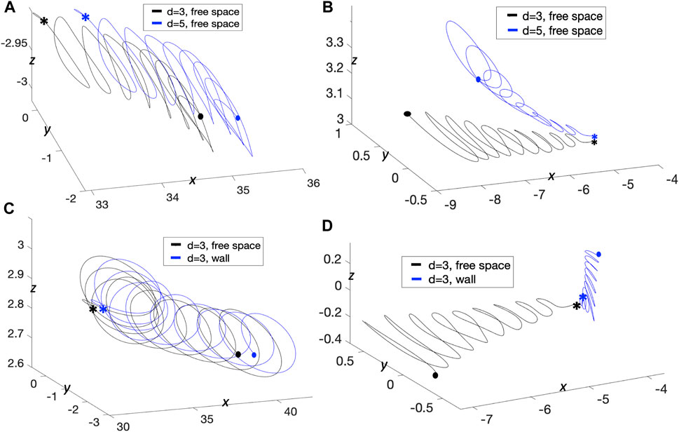
FIGURE 8. Trajectories with Parallel Sperm. Resulting trajectories for passive fluid markers as a result of the motion of sperm initialized in parallel planes with preferred planar beat forms. (A,B) Free space case with swimmers initialized d = 3, 5 μm apart. Initial locations of fluid markers in (A) are (33, 0, −2.9) and (33.6, 0, −2.9) and initialized at (−4.8, 0, 3.02) and (−4.8, 0, 3.04) in (B), for t = 0–0.4775 s. (C,D) Comparing trajectories with and without a wall with swimmers initialized d = 3 μm apart. Initial locations of fluid markers in (C) are (32.84, 0, 2.82) and (33.28, 0, 2.82) and initialized at (−4.2, 0, −0.1) and (−4.12, 0, −0.04) in (D), for t = 0–0.4325 s. Starting locations are denoted with * and ending locations are denoted with •.
Everything presented thus far has been for swimmers with a planar preferred beat form. Due to interactions with a swimmer or the wall, nonplanar beat forms have emerged (e.g., Figure 7D). Since different species of sperm exhibit a variety of nonplanar beat forms [2, 9], we now consider here the case of two quasi-planar swimmers where α = 3 μm and β = 1 μm in the preferred beat form in Eq. 3. The bottom swimmer is initialized with its centerline lying on the plane z = 0 and the top swimmer’s centerline is on the plane z = d.
We now wish to further characterize interactions of two swimmers with quasi-planar beat forms and understand how they are similar or different to swimmers with planar beat forms. In Figure 9, for an initial distance d = 6 μm apart, the two swimmer’s trajectories rotate around each other creating a bundle formed by the two flagella. At the same time, the two swimmers are attracting to each other, as shown in Figure 9B, where all distance metrics considered are oscillating and decreasing in time. Here, there are no signs of repulsion between the swimmers as they reach a minimum distance between the swimmers on the order of 3–4 μm for t ∈ [4, 5]s, similar to the swimmers with planar beat forms that were initialized as co-planar in Figure 2B and in contrast to those initialized in parallel planes in Figures 6A,E where repulsion was observed when starting d = 3, 5 μm apart. For the quasi-planar case, as expected, the trace of the first point shown in the zoomed portions of Figure 9A exhibit a more complicated trajectory, known as the flagelloid curve (or f-curve), as previously recorded in experiments and simulations for a single sperm [32, 39, 58, 59]. The flagelloid curve is shown in the yz-plane over the time interval from 2 to 3.2 s, where the curvature is higher at the bottom of the bundle and lower at the top of the bundle; this trend in curvature is consistent for the full time of the simulation.
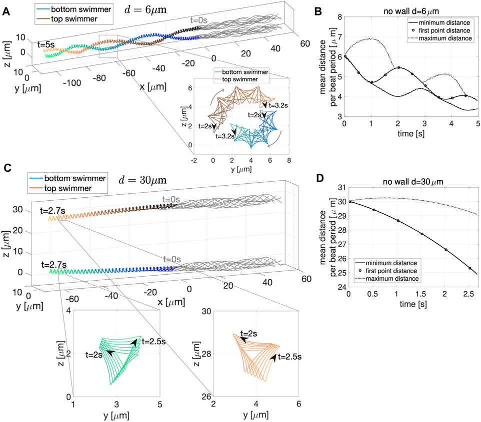
FIGURE 9. Quasi-Planar Swimmers in Free Space. 3D flagellar configurations for the first beat period (gray lines) and the trajectory of the first point in the direction of swimming (colored lines with respect to time) over the specified time interval for the two swimmers, initialized at a distance d = 6 μm apart in (A) and d = 30 μm apart in (C). The curves traced by the first point of the two swimmers on the yz-plane over the specified time interval are shown in the corresponding zoomed-in portions. Minimum (solid line) and maximum (dotted line) distance between the two swimmers and distance between the first points (circles) with respect to time for initial distance d = 6 μm in (B) and d = 30 μm in (D) (averages over a beat period).
We have also considered the case of two quasi-planar swimmers initialized at a distance of d = 30 μm in Figure 9C. In this case, the swimmer’s trajectories show clear attraction between the swimmers. That is, the minimum distance between the swimmers in Figure 9D is monotonically decreasing. Here, the average minimum distance and the average distance between the first points coincide for the full simulation. The flagelloid curves for d = 30 μm are also reported in the zoomed in portions of Figure 9C and exhibit a similar pattern to those in the zoomed in portions of Figure 9A.
The results reported in Figure 9 suggest that the fundamental dynamics in free space of two quasi-planar swimmers, in terms of attraction and repulsion, is similar to the dynamics of two co-planar swimmers reported in Section 3.1.1 and Figure 2. We also quantified the swimming speeds of a solo quasi-planar swimmer as well as a pair of quasi-planar swimmers (Table 2). Again, similar to the dynamics of attraction, the swimming speed trends were similar to that of the co-planar swimmers. Relative to the swimming speed of a solo swimmer, a pair of swimmers 5 μm apart had a decrease in swimming speed whereas swimmers initially 30 μm apart had a very small increase in swimming speed (at earlier time points). For the preferred configurations studied, the quasi-planar swimmers were slower than the planar swimmers (by a few μm/s). We also emphasize that no difference in the results are obtained if the second swimmer was initialized with a centerline lying on the plane y = d, instead of z = d, i.e., translating on the y-axis instead of the z-axis.
Figure 10A shows the dynamics near a planar wall for a pair of swimmers initialized a distance d = 6 μm apart; the two swimmers attract to the wall and start rotating around each other. Similar to the free space case in Figure 9A, the swimmers continue to circle each other. However, with the wall in Figure 10A, they do not progress forward but stay a constant distance away from the wall, remaining perpendicular to the wall. The zoomed portion of Figure 10A shows the flagelloid curves traced by the first point on the swimmers. The curvature is approximately the same whether the swimmer is at the top or at the bottom of the bundle. This trend in curvature is consistent for the full time of the simulation and in contrast to quasi-planar swimmers in free space (Figures 9A,C). In terms of the dynamics of attraction, after an initial transient period of approximately 1 s where the first points of the swimmer attract and then repulse, the swimmers reach an almost-constant average distance between the heads at ∼6 μm apart (Figure 10C). Similarly, swimmers initialized 3 μm apart reach a constant distance apart around 1 s, but the heads repulse initially and level off at a distance ∼5 μm apart (Figure 10B).
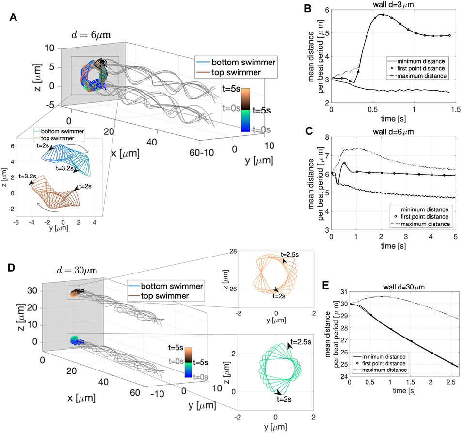
FIGURE 10. Quasi-Planar Swimmers Near a Wall. 3D flagellar configurations for the first beat period (gray lines) and the trajectory of the first point in the direction of swimming (colored lines with respect to time) over the time interval from 0 to 5 s for the two swimmers, initialized at a distance d = 6 μm in (A) and d = 30 μm in (D) near a wall at x = −5 μm. The curves traced by the first point of the two swimmers on the yz-plane over the specified time interval are shown in the corresponding zoomed-in portions. Minimum (solid line) and maximum (dotted line) distance between the two swimmers and distance between the first points of the two swimmers (circles) with respect to time for initial distance d = 3 μm in (B), d = 6 μm in (C), and d = 30 μm in (E) (distances averaged over a beat period). The gray panel in (A,D) represents the wall.
The case of two quasi-planar swimmers initialized at a distance of 30 μm apart and also near the wall at x = −5 is shown in Figure 10D. In this case, the swimmer’s trajectories show clear attraction, i.e., monotonic decrease of the average minimum distance between the swimmers (Figure 10E). The results reported in Figure 10 suggest that the fundamental dynamics near a wall of two quasi-planar swimmers, in terms of attraction and repulsion, is similar to the dynamics of two co-planar swimmers near a wall reported in Section 3.1.1 and Figure 3. In particular, we point out the strong similarity between Figures 3D–F and Figures 10B,C,E. We also emphasize that no difference in the results were obtained if the second swimmer was initialized with a centerline lying on the plane y = d, instead of z = d.
The ability of mammalian sperm to reach and fertilize the egg is aided by a multitude of dynamic interactions between swimmers, signaling molecules in the fluid, and walls of the female reproductive tract. In this work, we provide a detailed look at pairs of swimmers to characterize conditions that lead to emergent phenomena such as attraction or repulsion of swimmers. In free space, we observe long-term attraction of two swimmers in the case of initially co-planar sperm with preferred planar beat forms and sperm initially with centerlines in parallel planes with preferred quasi-planar beat forms. In contrast, sperm initially with centerlines in parallel planes and preferred planar beat forms exhibit oscillatory dynamics, alternating between periods of attraction and repulsion. For both of these, we emphasize that these classifications are for separation distances on a length scale smaller than the length of the flagella and greater than or equal to the beat amplitude. When sperm are swimming in close proximity to a wall, we observe attraction to the wall for planar and quasi-planar beat forms, i.e., even if swimmers are in close proximity when near the wall, they are still trapped at the wall. For sperm initialized in parallel planes with a planar preferred beat form and near a wall, due to the instability in the angle of the attracted swimmers, we observe significant rolling episodes that allow the swimmers to attain a beat form and distance apart that can then be maintained. The observation of this rolling behavior is important as it is proposed to be an important mechanism in sperm selection [56].
The results presented in this work further clarify and contextualize divergent results in the literature. For example, in the case of parallel sperm in free space, our far-field attraction results differ from previous results of [26] where only repulsion was observed and [31] where only attraction is observed. We are able to show that the swimmers in this configuration will not reach a stable configuration of attraction and will continue to oscillate between attraction and repulsion. Zooming in on a particular time frame and/or different parameter choice leads to these divergent behaviors. Understanding the complex interactions of beat form and elasticity of the flagella can also be utilized to design artificial micro-swimmers that navigate in complex environments [35–37].
The modeling framework used did not account for background fluid flows and limited the study to the case of two swimmers initialized in the same plane or with centerlines in parallel planes. In all of the cases where attraction is observed, we emphasize that perturbations to the flow would likely cause additional rolling and pitching. Similarly, we focused on the case of a purely homogeneous fluid with a constant viscosity. It is well known that the viscosity of the fluid in the female reproductive tract varies and will often exhibit nonlinear properties with respect to stress and strain [2, 10]. We observed changes in the dynamics of attraction with increases in the viscosity and hence, we expect that nonhomogeneous or nonlinear fluid contributions will also act to change the frequency of rolling and the degree of pitching in the swimmers. This will be the focus of future studies.
The raw data supporting the conclusions of this article will be made available by the authors, without undue reservation.
LC and SO conceptualized this research and completed the writing. LC and DD completed simulations and created figures. All authors have contributed to this article and have given approval for this submission.
The work of SDO and DD was supported, in part, by NSF DMS 1455270. SDO was also supported, in part, by the Fulbright Research Scholar Program. Simulations were run on a cluster at WPI acquired through NSF grant 1337943 and on a cluster provided by Research Computing at the Rochester Institute of Technology (60).
The authors declare that the research was conducted in the absence of any commercial or financial relationships that could be construed as a potential conflict of interest.
All claims expressed in this article are solely those of the authors and do not necessarily represent those of their affiliated organizations, or those of the publisher, the editors and the reviewers. Any product that may be evaluated in this article, or claim that may be made by its manufacturer, is not guaranteed or endorsed by the publisher.
1. Dcunha R, Hussein R, Ananda H, Kumari S, Adiga S, Kannan N, et al. Current Insights and Latest Updates in Sperm Motility and Associated Applications in Assisted Reproduction. Reprod Sci (2020) [Epub ahead of print] 1–19. doi:10.1007/s43032-020-00408-y
2. Gaffney EA, Gadêlha H, Smith DJ, Blake JR, Kirkman-Brown JC. Mammalian Sperm Motility: Observation and Theory. Annu Rev Fluid Mech (2011) 43:501–28. doi:10.1146/annurev-fluid-121108-145442
3. Alavi S, Cosson J. Sperm Motility in Fishes. (II) Effects of Ions and Osmolality: a Review. Cel Biol Int (2006) 30:1–14. doi:10.1016/j.cellbi.2005.06.004
4. Suarez SS, Pacey AA. Sperm Transport in the Female Reproductive Tract. Hum Reprod Update (2006) 12:23–37. doi:10.1093/humupd/dmi047
5. Suarez SS. Regulation of Sperm Storage and Movement in the Mammalian Oviduct. Int J Dev Biol (2008) 52:455–62. doi:10.1387/ijdb.072527ss
6. Elgeti J, Winkler RG, Gompper G. Physics of Microswimmers-Single Particle Motion and Collective Behavior: a Review. Rep Prog Phys (2015) 78:056601. doi:10.1088/0034-4885/78/5/056601
7. Schoeller SF, Keaveny EE. From Flagellar Undulations to Collective Motion: Predicting the Dynamics of Sperm Suspensions. J R Soc Interf (2018) 15:20170834. doi:10.1098/rsif.2017.0834
8. Schoeller SF, Holt WV, Keaveny EE. Collective Dynamics of Sperm Cells. Phil Trans R Soc B (2020) 375:20190384. doi:10.1098/rstb.2019.0384
9. Guerrero A, Carneiro J, Pimentel A, Wood CD, Corkidi G, Darszon A. Strategies for Locating the Female Gamete: the Importance of Measuring Sperm Trajectories in Three Spatial Dimensions. Mol Hum Reprod (2011) 17:511–23. doi:10.1093/molehr/gar042
10. Smith DJ, Gaffney EA, Gadêlha H, Kapur N, Kirkman-Brown JC. Bend Propagation in the Flagella of Migrating Human Sperm, and its Modulation by Viscosity. Cell Motil. Cytoskeleton (2009) 66:220–36. doi:10.1002/cm.20345
11. Woolley DM, Vernon GG. A Study of Helical and Planar Waves on Sea Urchin Sperm Flagella, with a Theory of How They Are Generated. J Exp Biol (2001) 204:1333–45. doi:10.1242/jeb.204.7.1333
12. Su TW, Xue L, Ozcan A. High-throughput Lensfree 3D Tracking of Human Sperms Reveals Rare Statistics of Helical Trajectories. Proc Natl Acad Sci U S A (2012) 109:16018–22. doi:10.1073/pnas.1212506109
13. Su T-W, Choi I, Feng J, Huang K, McLeod E, Ozcan A. Sperm Trajectories Form Chiral Ribbons. Sci Rep (2013) 3:1664. doi:10.1038/srep01664
14. Lauga E, Powers TR. The Hydrodynamics of Swimming Microorganisms. Rep Prog Phys (2009) 72:096601. doi:10.1088/0034-4885/72/9/096601
15. Ardon F, Markello RD, Hu L, Deutsch ZI, Tung CK, Wu M, et al. Dynamics of Bovine Sperm Interaction with Epithelium Differ between Oviductal Isthmus and Ampulla. Biol Reprod (2016) 95:90–7. doi:10.1095/biolreprod.116.140632
16. Lamy J, Corbin E, Blache M-C, Garanina AS, Uzbekov R, Mermillod P, et al. Steroid Hormones Regulate Sperm-Oviduct Interactions in the Bovine. Reprod (2017) 154:497–508. doi:10.1530/rep-17-0328
17. Ramal-Sanchez M, Bernabo N, Tsikis G, Blache M-C, Labas V, Druart X, et al. Progesterone Induces Sperm Release from Oviductal Epithelial Cells by Modifying Sperm Proteomics, Lipidomics and Membrane Fluidity. Mol Cell Endocrinol (2020) 504:110723. doi:10.1016/j.mce.2020.110723
18. Curtis MP, Kirkman-Brown JC, Connolly TJ, Gaffney EA. Modelling a Tethered Mammalian Sperm Cell Undergoing Hyperactivation. J Theor Biol (2012) 309:1–10. doi:10.1016/j.jtbi.2012.05.035
19. Simons J, Olson S, Cortez R, Fauci L. The Dynamics of Sperm Detachment from Epithelium in a Coupled Fluid-Biochemical Model of Hyperactivated Motility. J Theor Biol (2014) 354:81–94. doi:10.1016/j.jtbi.2014.03.024
20. Wang S, Larina IV. In Vivo three-dimensional Tracking of Sperm Behaviors in the Mouse Oviduct. Development (2018) 145:dev157685. doi:10.1242/dev.157685
21. Camara Pirez M, Steele H, Reese S, Kölle S. Bovine Sperm-Oviduct Interactions Are Characterized by Specific Sperm Behaviour, Ultrastructure and Tubal Reactions Which Are Impacted by Sex Sorting. Sci Rep (2020) 10:16522. doi:10.1038/s41598-020-73592-1
22. Denissenko P, Kantsler V, Smith DJ, Kirkman-Brown J. Human Spermatozoa Migration in Microchannels Reveals Boundary-Following Navigation. Proc Natl Acad Sci U S A (2012) 109:8007–10. doi:10.1073/pnas.1202934109
23. Tung C-k., Ardon F, Fiore AG, Suarez SS, Wu M. Cooperative Roles of Biological Flow and Surface Topography in Guiding Sperm Migration Revealed by a Microfluidic Model. Lab Chip (2014) 14:1348–56. doi:10.1039/c3lc51297e
24. Llopis I, Pagonabarraga I, Lagomarsino MC, Lowe C. Cooperative Motion of Intrinsic and Actuated Semiflexible Swimmers. Phys Rev E (2013) 87:032720. doi:10.1103/physreve.87.032720
25. Olson SD, Fauci LJ. Hydrodynamic Interactions of Sheets vs Filaments: Synchronization, Attraction, and Alignment. Phys Fluids (2015) 27:121901. doi:10.1063/1.4936967
26. Simons J, Fauci L, Cortez R. A Fully Three-Dimensional Model of the Interaction of Driven Elastic Filaments in a Stokes Flow with Applications to Sperm Motility. J Biomech (2015) 48:1639–51. doi:10.1016/j.jbiomech.2015.01.050
27. Miki K, Clapham DE. Rheotaxis Guides Mammalian Sperm. Curr Biol (2013) 23:443–52. doi:10.1016/j.cub.2013.02.007
28. Ishimoto K, Gaffney EA. Fluid Flow and Sperm Guidance: a Simulation Study of Hydrodynamic Sperm Rheotaxis. J R Soc Interf (2015) 12:20150172. doi:10.1098/rsif.2015.0172
29. Gillies EA, Cannon RM, Green RB, Pacey AA. Hydrodynamic Propulsion of Human Sperm. J Fluid Mech (2009) 625:445–74. doi:10.1017/s0022112008005685
30. Smith DJ, Gaffney EA, Blake JR, Kirkman-Brown JC. Human Sperm Accumulation Near Surfaces: a Simulation Study. J Fluid Mech (2009) 621:289–320. doi:10.1017/s0022112008004953
31. Walker B, Ishimoto K, Gaffney E. Pairwise Hydrodynamic Interactions of Synchronized Spermatozoa. Phys Rev Fluids (2019) 4:093101. doi:10.1103/physrevfluids.4.093101
32. Ishimoto K, Gaffney EA. An Elastohydrodynamical Simulation Study of Filament and Spermatozoan Swimming Driven by Internal Couples. IMA J Appl Math (2018) 83:655–79. doi:10.1093/imamat/hxy025
33. Yang Y, Elgeti J, Gompper G. Cooperation of Sperm in Two Dimensions: Synchronization, Attraction, and Aggregation through Hydrodynamic Interactions. Phys Rev E Stat Nonlin Soft Matter Phys (2008) 78:061903. doi:10.1103/PhysRevE.78.061903
34. Huang J, Carichino L, Olson SD. Hydrodynamic Interactions of Actuated Elastic Filaments Near a Planar wall with Applications to Sperm Motility. J Coupled Syst Multiscale Dyn (2018) 6:163–75. doi:10.1166/jcsmd.2018.1166
35. Gao W, Wang J. Synthetic Micro/nanomotors in Drug Delivery. Nanoscale (2014) 6:10486–94. doi:10.1039/c4nr03124e
36. Nelson BJ, Kaliakatsos IK, Abbott JJ. Microrobots for Minimally Invasive Medicine. Annu Rev Biomed Eng (2010) 12:55–85. doi:10.1146/annurev-bioeng-010510-103409
37. Sanders L. Microswimmers Make a Splash: Tiny Travelers Take on a Viscous World. Sci News (2009) 176:22–5. doi:10.1002/scin.5591760124
38. Fauci LJ, Dillon R. Biofluidmechanics of Reproduction. Annu Rev Fluid Mech (2006) 38:371–94. doi:10.1146/annurev.fluid.37.061903.175725
39. Carichino L, Olson SD. Emergent Three-Dimensional Sperm Motility: Coupling Calcium Dynamics and Preferred Curvature in a Kirchhoff Rod Model. Math Med Biol (2019) 36:439–69. doi:10.1093/imammb/dqy015
40. Lim S, Ferent A, Wang XS, Peskin CS. Dynamics of a Closed Rod with Twist and bend in Fluid. SIAM J Sci Comput (2008) 31:273–302. doi:10.1137/070699780
41. Lim S. Dynamics of an Open Elastic Rod with Intrinsic Curvature and Twist in a Viscous Fluid. Phys Fluids (2010) 22:024104. doi:10.1063/1.3326075
42. Olson SD, Lim S, Cortez R. Modeling the Dynamics of an Elastic Rod with Intrinsic Curvature and Twist Using a Regularized Stokes Formulation. J Comput Phys (2013) 238:169–87. doi:10.1016/j.jcp.2012.12.026
43. Schmitz-Lesich KA, Lindemann CB. Direct Measurement of the Passive Stiffness of Rat Sperm and Implications to the Mechanism of the Calcium Response. Cel Motil. Cytoskeleton (2004) 59:169–79. doi:10.1002/cm.20033
44. Olson SD, Suarez SS, Fauci LJ. Coupling Biochemistry and Hydrodynamics Captures Hyperactivated Sperm Motility in a Simple Flagellar Model. J Theor Biol (2011) 283:203–16. doi:10.1016/j.jtbi.2011.05.036
45. Chouaieb N, Maddocks JH. Kirchhoff's Problem of Helical Equilibria of Uniform Rods. J Elasticity (2004) 77:221–47. doi:10.1007/s10659-005-0931-z
46. Chouaieb N, Goriely A, Maddocks JH. Helices. Proc Natl Acad Sci (2006) 103:9398–403. doi:10.1073/pnas.0508370103
47. Woolley DM. Flagellar Oscillation: a Commentary on Proposed Mechanisms. Biol Rev Camb Philos Soc (2010) 85:453–70. doi:10.1111/j.1469-185X.2009.00110.x
48. Cortez R. The Method of Regularized Stokeslets. SIAM J Sci Comput (2001) 23:1204–25. doi:10.1137/s106482750038146x
49. Cortez R, Fauci L, Medovikov A. The Method of Regularized Stokeslets in Three Dimensions: Analysis, Validation, and Application to Helical Swimming. Phys Fluids (2005) 17:0315041. doi:10.1063/1.1830486
50. Ainley J, Durkin S, Embid R, Boindala P, Cortez R. The Method of Images for Regularized Stokeslets. J Comput Phys (2008) 227:4600–16. doi:10.1016/j.jcp.2008.01.032
51. Cortez R, Varela D. A General System of Images for Regularized Stokeslets and Other Elements Near a Plane wall. J Comput Phys (2015) 285:41–54. doi:10.1016/j.jcp.2015.01.019
52. Eberly D. Least Squares Fitting of Data (Version February 14, 2019). Chapel Hill, NC: Magic Software (2000).
53. Woolley DM, Crockett RF, Groom WDI, Revell SG. A Study of Synchronisation between the Flagella of Bull Spermatozoa, with Related Observations. J Exp Biol (2009) 212:2215–23. doi:10.1242/jeb.028266
54. Hunter RHF, Coy P, Gadea J, Rath D. Considerations of Viscosity in the Preliminaries to Mammalian Fertilisation. J Assist Reprod Genet (2011) 28:191–7. doi:10.1007/s10815-010-9531-3
55. Kirkman-Brown JC, Smith DJ. Sperm Motility: Is Viscosity Fundamental to Progress? Mol Hum Reprod (2011) 17:539–44. doi:10.1093/molehr/gar043
56. Babcock DF, Wandernoth PM, Wennemuth G. Episodic Rolling and Transient Attachments Create Diversity in Sperm Swimming Behavior. BMC Biol (2014) 12:67. doi:10.1186/s12915-014-0067-3
57. Gadêlha H, Hernández-Herrera P, Montoya F, Darszon A, Corkidi G. Human Sperm Uses Asymmetric and Anisotropic Flagellar Controls to Regulate Swimming Symmetry and Cell Steering. Sci Adv (2020) 6:eaba5168. doi:10.1126/sciadv.aba5168
58. Woolley D. Motility of Spermatozoa at Surfaces. Reprod (2003) 126:259–70. doi:10.1530/rep.0.1260259
59. Woolley DM. Studies on the Eel Sperm Flagellum. 2. The Kinematics of normal Motility. Cel Motil. Cytoskeleton (1998) 39:233–45. doi:10.1002/(sici)1097-0169(1998)39:3<233::aid-cm6>3.0.co;2-5
Keywords: method of regularized stokeslets, sperm motility, hydrodynamic interactions, image systems, quasi-planar beatforms, collective motion
Citation: Carichino L, Drumm D and Olson SD (2021) A Computational Study of Hydrodynamic Interactions Between Pairs of Sperm With Planar and Quasi-Planar Beat Forms. Front. Phys. 9:735438. doi: 10.3389/fphy.2021.735438
Received: 02 July 2021; Accepted: 27 September 2021;
Published: 01 November 2021.
Edited by:
Laura Ann Miller, University of Arizona, United StatesReviewed by:
Charles Wolgemuth, University of Arizona, United StatesCopyright © 2021 Carichino, Drumm and Olson. This is an open-access article distributed under the terms of the Creative Commons Attribution License (CC BY). The use, distribution or reproduction in other forums is permitted, provided the original author(s) and the copyright owner(s) are credited and that the original publication in this journal is cited, in accordance with accepted academic practice. No use, distribution or reproduction is permitted which does not comply with these terms.
*Correspondence: Lucia Carichino, bGNzbWExQHJpdC5lZHU=
Disclaimer: All claims expressed in this article are solely those of the authors and do not necessarily represent those of their affiliated organizations, or those of the publisher, the editors and the reviewers. Any product that may be evaluated in this article or claim that may be made by its manufacturer is not guaranteed or endorsed by the publisher.
Research integrity at Frontiers
Learn more about the work of our research integrity team to safeguard the quality of each article we publish.