A Novel Cell Vertex Model Formulation that Distinguishes the Strength of Contraction Forces and Adhesion at Cell Boundaries

The vertex model is a useful mathematical model to describe the dynamics of epithelial cell sheets. However, existing vertex models do not distinguish contraction forces on the cell boundary from adhesion between cells, employing a single parameter to express both. In this paper, we introduce the rest length of the cell boundary and its dynamics into the existing vertex model, giving a novel formulation of the model that treats separately the contraction force and the strength of adhesion between cells. We apply this vertex model to the phenomenon of compartment boundary in the fruit fly pupa, recapturing the observation that increasing the strength of adhesion between cells straightens the compartment boundary, even though contraction forces at cell boundaries remain unchanged. We also discuss possibilities of the novel vertex models by considering the stretching of a cell sheet by external forces.

Introduction

During embryonic development, epithelial cells form a monolayer sheet that covers the entire embryo. Cells comprising the sheet move drastically, like an active viscoelastic fluid, while maintaining their attachment to adjacent cells. This spontaneous movement of epithelial cells is considered a driving force for morphogenesis of multicellular organisms. Understanding the mechanism of the movement from not only a molecular but also a mechanical point of view is a challenging problem in morphogenesis. Although the molecular mechanism of the movement has come to be relatively well understood [1], its mechanical mechanism is still an ongoing problem.

To approach the mechanical mechanism of the dynamics of the epithelial sheet, a cell-based mathematical model, the vertex model, is often used [2, 3]. In this model, each epithelial cell in the sheet is expressed by a polygon, and the cell configuration within the sheet is completely specified by the positions of the vertices of the polygons. The vertex model can describe various aspects of the epithelial sheet at the cellular level, including mechanical forces generated by each cell and the planar polarities of cells [2, 3]. Indeed, by using the vertex model, important behaviors of the epithelial sheet, such as elongation, bending, and unidirectional movement of the sheet, have been explained from not only a biological but also a mechanical viewpoint [4–7].

Although the existing vertex model is well able to describe important properties of epithelial cell sheets, certain modifications are necessary in order to more precisely describe cell sheet dynamics. One important consideration is the lack of distinction between the contraction forces acting on the cell boundaries and the adhesion between cells. The existing vertex models consider the contraction forces and the strength of adhesion together and express the strengths of these two factors using a single parameter [8, 9]. However, biologically, contraction and adhesion are regulated by different molecules. For example, contraction forces are generated by actomyosin networks beneath the plasma membrane, whereas adhesion between cells is accomplished by adhesion molecules such as cadherin. Hence, to make the vertex model more useful and to more precisely describe epithelial cell sheet dynamics, it is preferable to modify the existing model to separately treat the forces of contraction and adhesion at the cell boundaries.

In this paper, we provide a novel formulation of the vertex model that introduces a phenomenological variable corresponding to the rest length of a cell boundary. This formulation allows us to treat separately the contraction forces acting on cell boundaries and the effects of adhesion between cells. The vertex model presented here is in accordance with and an extension of the existing vertex model. As an application of the model presented in this paper, we consider a phenomenon observed in the anterior-posterior (AP) compartment boundary in the Drosophila pupa [10, 11], in which the AP compartment boundary is straightened not only by an increase in contraction force at this boundary but also by an increase in the strength of adhesion between cells in the posterior region. While it has been demonstrated that the increase in contraction forces at the AP compartment boundary straightens the boundary [10], it has not yet been demonstrated whether the increase in adhesion between posterior cells does likewise. We use the vertex model presented here to show that the increase in adhesion between cells in the posterior region does straighten the AP compartment boundary and explain why the increase in adhesion straightens the boundary. As a second application of the new vertex model, we focus on stretching of the epithelial sheet by an external force. This application illustrates the difference in cell remodeling behavior between existing vertex models and our new model and compares the results predicted by the models with those observed experimentally.

Setup of the Vertex Model

As in existing vertex models, cells comprising an epithelial sheet are represented by polygons. The mechanical forces generated by the cells are expressed by the potential function $U$:

$U=\frac{K}{2}{\displaystyle \sum _{\mathrm{cell}\alpha }{\left(A_{\alpha }-A_{\alpha }^{\left(0\right)}\right)}^2}+{\displaystyle \sum _{\langle ij\rangle }{\gamma }_{ij}{\ell }_{ij}}+\frac{k}{2}{\displaystyle \sum _{\langle ij\rangle }{\left({\ell }_{ij}-{\ell }_{ij}^{\left(M\right)}\right)}^2},(1)$

where $A_{\alpha }$ is the area of the α^th cell, $A_{\alpha }^{\left(0\right)}$ is its preferred value, $K$ and $k$ are positive constants, and ${\ell }_{ij}$ is the length of cell boundary $ij$ that connects the $i^{th}$ and $j^{th}$ vertices. The index α includes all cells in the cell sheet, and $\langle ij\rangle$ below the summation symbol implies that index $ij$ includes all cell boundaries in the system. A point of difference of this model compared with previous ones is the third term in Eq. 1. The first term in Eq. 1 represents cytosolic hydrostatic pressure that acts on the cell boundaries. The second term in Eq. 1 represents the contraction force acting on the cell boundary $ij$, which comes from the cortical actomyosin network beneath the plasma membrane. In this model, ${\gamma }_{ij}$ represents only the strength of the contraction force and does not include the strength of adhesion between cells; the strength of adhesion will be expressed by ${\tau }_{ij}$ in Eq. 3. The novel third term in Eq. 1 represents phenomenological forces acting on cell boundaries, which are introduced by considering the rest length (natural length) of cell boundary $ij$, denoted by ${\ell }_{ij}^{\left(M\right)}$. The introduction of this last term is based on the following considerations. The cell boundary consists of materials such as membrane, cytoskeleton, and associated components. In our model, we symbolically describe the amount of these cell boundary components by ${\ell }_{ij}^{\left(M\right)}$. Since ${\ell }_{ij}^{\left(M\right)}$ has the dimension of length, this quantity is obtained by dividing the amount of the cell boundary components by some constant having the dimensions of (amount of components)/(length). If the amount of the materials at cell boundary ij is greater than the appropriate amount of the materials for making the boundary with length ${\ell }_{ij}$, the excess of the materials may give rise to repulsive forces by showing the wriggle of membrane. On the other hand, if the amount of material comprising the cell boundary ij is less than the appropriate value for the length ${\ell }_{ij}$, where the distances between the components comprising the cell boundary, such as lipid molecules, are large, an attractive force may arise to return these components to the equilibrium positions. These tendencies of the force on the cell boundary are expressed by the third term in Eq. 1. The quantity ${\ell }_{ij}^{\left(M\right)}$ is a variable that evolves with time, as given by Eq. 3.

In the previous vertex models [2, 7, 9], there is another term in $U$, which is a quadratic term of cell perimeter, expressed by $\frac{K_p}{2}{\displaystyle \sum _{\mathrm{cell}\alpha }{\left(L_{\alpha }-L_0\right)}^2}$ (see Supplementary Appendix 1), where $L_{\alpha }$ is the perimeter of cell α, and $K_p$ and $L_0$ are constants. This term serves to express the conservation of the amount of cell membrane, or the effect of quadratic terms of cell perimeter, into the cell sheet dynamics. Our model, however, does not include this term in $U$, because an equivalent effect is included in Eq. 3.

The total mechanical force acting on vertex $i$ is given by $-\partial U/\partial {\mathbf{r}}_i$, where ${\mathbf{r}}_{\mathit{i}}$ is the position of the ith vertex, ${\mathbf{r}}_{\mathit{i}}=\left(x_i,y_i\right)$. We set up the model such that the positions of all vertices in the sheet move in such a way that the total mechanical force on each vertex must sum to zero at any time, i.e.,

$-\frac{\partial U}{\partial {\mathbf{r}}_{\mathit{i}}}=0(2)$

holds for all vertices $i$ at any time t. This situation corresponds to the case where we consider the cell sheet dynamics on a relatively longer time scale, such as minutes or tens of minutes. For the practical implementation of Eq. 2, it is useful to solve $\eta \frac{d{\mathbf{r}}_{\mathit{i}}}{dt}=-\frac{\partial U}{\partial {\mathbf{r}}_{\mathit{i}}}$ with an extremely small positive value of $\eta$. In this implementation, the vertex positions obtained are nearly independent of the value of $\eta$, when $\eta$ is taken to be sufficiently small.

Next, we consider the time evolution equation for ${\ell }_{ij}^{\left(M\right)}$. As mentioned above, the quantity ${\ell }_{ij}^{\left(M\right)}$ corresponds to the amount of materials comprising cell boundary ij, so that the rate of change in ${\ell }_{ij}^{\left(M\right)}$ is related to the rate of change in the amount of these materials. For example, it depends on the rate of turnover of cell membrane at the boundary, which relates to the frequency of membrane endocytosis [12] and exocytosis at the cell boundary. Hereafter we refer to the ability to change the amount of cell boundary components as the “activity of the cell boundary”. In addition, ${\ell }_{ij}^{\left(M\right)}$ tends to approach ${\ell }_{ij}$ over time, because if the amount of cell boundary components is not appropriate for length ${\ell }_{ij}$, the amount tries to approach the appropriate value. The speed at which ${\ell }_{ij}^{\left(M\right)}$ approaches ${\ell }_{ij}$ may depend on the activity of the cell boundary. Furthermore, the total sum of ${\ell }_{ij}^{\left(M\right)}$ in each cell tends to be conserved over the timescale considered here, because the creation and destruction of components of cell membrane are modest within periods of minutes or several tens of minutes [13]. Considering these properties of the dynamics of cell boundary components, we determine the time evolution equation for ${\ell }_{ij}^{\left(M\right)}$ as

$\frac{d{\ell }_{ij}^{\left(M\right)}}{dt}=-\frac{1}{{\tau }_{ij}}\left({\ell }_{ij}^{\left(M\right)}-{\ell }_{ij}\right)-\frac{\partial M}{\partial {\ell }_{ij}^{\left(M\right)}},(3)$

where ${\tau }_{ij}$ is a relaxation time that expresses the rate of approach of ${\ell }_{ij}^{\left(M\right)}$ to ${\ell }_{ij}$. In this model, ${\tau }_{ij}$ is assumed to depend on the activity of cell boundary $ij$. $M$ is a function of $\left\{{\ell }_{ij}^{\left(M\right)}\right\}$ that expresses the tendency to conserve the sum of ${\ell }_{ij}^{\left(M\right)}$ for each cell, given as

$M=\frac{k_{pm}}{2}{\displaystyle \sum _{\mathrm{c}\mathrm{e}\mathrm{l}\mathrm{l}\mathrm{\alpha }}{\left(\left({\displaystyle \sum _{klin\mathrm{c}\mathrm{e}\mathrm{l}\mathrm{l}\mathrm{\alpha }}{\ell }_{kl}^{\left(M\right)}}\right)-L_{\alpha }^{\left(0\right)}\right)}^2},(4)$

where $k_{pm}$ is a positive constant expressing the degree of tendency to conserve the junction rest lengths. $L_{\alpha }^{\left(0\right)}$ is a positive constant corresponding to the total amount of cell boundary components in the α^th cell. The sign “kl in cell α” under the summation symbol signifies that the sum is taken over all boundaries of cell α.

As stated above, the quantity ${\tau }_{ij}$ in Eq. 3 expresses the inverse of the rate at which ${\ell }_{ij}^{\left(M\right)}$ approaches ${\ell }_{ij}$. That is, when ${\tau }_{ij}$ is large, ${\ell }_{ij}^{\left(M\right)}$ approaches ${\ell }_{ij}$ slowly, and vice versa. Experimental results indicate that the rate of cell membrane turnover can differ from one cell boundary to another, due to planar polarized endocytic activity [14]. In addition, the rate of endocytosis at a cell boundary is related to the degree of adhesion at the boundary [14], i.e., when endocytosis at the cell boundary is frequent, adhesion between the cells sharing the boundary is weakened, and vice versa. Thus, in this model we interpret that the state where ${\tau }_{ij}$ is large is a state at which the adhesion at cell boundary ij is strong, and vice versa. If we accept this setup, we can distinguish contraction force acting on the cell boundary from the strength of adhesion at the boundary, namely, the contraction on cell boundary ij is expressed by ${\gamma }_{ij}$ in Eq. 1 (large ${\gamma }_{ij}$ indicating strong contraction on cell boundary ij), while the strength of adhesion at cell boundary ij is expressed by ${\tau }_{ij}$ in Eq. 3 (large ${\tau }_{ij}$ indicating strong adhesion at this boundary).

Application 1: Straightening of Compartment Boundary in Developing Fruit fly Pupa

Numerical Demonstrations that the Increase in ${\tau }_{ij}$ at Boundaries Between P Cells Shortens the Compartment Boundary

As an application of this new vertex model, we treat the phenomenon of compartment boundary straightening in the fruit fly pupa [15]. In this phenomenon, two types of epithelial cells, anterior (A) cells and posterior (P) cells, form two domains in an epithelial sheet, and the two cell domains meet at a boundary called the compartment boundary. For pupal development to progress correctly, the compartment boundary must undergo sufficient straightening. A mechanism that has been considered for the straightening of the compartment boundary is a strengthening of the contraction force on the compartment boundary, which shortens and straightens the compartment boundary. This scenario has been confirmed using the previous vertex model [10]. Recently, however, another mechanism for straightening of the compartment boundary was experimentally demonstrated [11], in which this boundary is straightened by an increase in the strength of adhesion between P cells, with the contraction force on the compartment boundary remaining unchanged. To restore this phenomenon, we used the new vertex model to try to understand why and how an increase in adhesion between P cells straightens the compartment boundary.

To do this, we set up the situation where a cell sheet consists of two types of cells, A cells (red) and P cells (blue) (Figure 1A). We refer to the boundary between the A and P cells as the compartment boundary in this model. As the initial state (t = 0) of the cell sheet, we took the equilibrium state obtained under the condition in which both A and P cells had the same parameters. Then at t = 0, we changed the parameters of interest and observed the length difference ($\Delta L$) of the compartment boundary between the initial state (t = 0) and the final state. Here, the final state is the steady state of the sheet under the new parameter values. If the result of numerical simulation exhibited $\Delta L<0$, the compartment boundary was shortened and straightened, or vice versa. First, to retrace the previous work [10], we increased the contraction forces (${\gamma }_{ij}$) at the compartment boundary at t = 0 in our model. The result of numerical simulation showed that $\Delta L<0$ in response to the increase in ${\gamma }_{ij}$ at compartment boundary (Figure 1B; Supplementary Movie 1). This result is reasonable because the large ${\gamma }_{ij}$ (strong contraction) at the compartment boundary pulls the vertices at the compartment boundary closer together, hence shortening and straightening the compartment boundary.

FIGURE 1

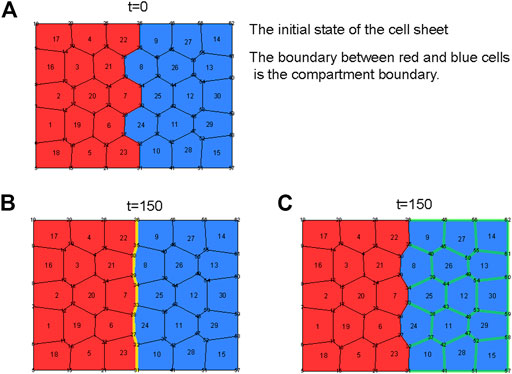
FIGURE 1. (A) The initial state of the cell sheet. Red and blue cells are anterior and posterior cells, respectively. At the initial state of the sheet, both cells have the same parameters. At time t = 0, some parameters are changed. The compartment boundary is the boundary between red and blue cells. (B) The final state of the cell sheet when ${\gamma }_{ij}$ at the compartment boundary is changed from ${\gamma }_{ij}=0.1$(default value) to ${\gamma }_{ij}=0.2$ (see Supplementary Movie 1). (C) The final state of the cell sheet when ${\tau }_{PP}$ at the cell boundary between P cells is changed from ${\tau }_{PP}=0.1$ (default value) to ${\tau }_{PP}=0.3$ (see Supplementary Movie 2). To highlight which cell boundary changed parameters, we colored them yellow (B) and green (C). The parameter values used here are $K=4$, $k=1$, $A_{\alpha }^{\left(0\right)}=2\text{.}2$, ${\gamma }_{ij}=0.1$ (default), $k_{pm}=5$, $\eta =0.01$, ${\tau }_{ij}=0.1$ (default), and $L_{\alpha }^{\left(0\right)}=1.2\times \left(2\pi \sqrt{A_{\alpha }^{\left(0\right)}/\pi }\right)=6.3$. For the units of these parameters see Supplementary Table 1.

Next, to investigate the effects on $\Delta L$ of a change in adhesion strength between cells, we changed the values of ${\tau }_{ij}$ at the cell boundaries between P cells at t = 0. In this simulation, we increased only the adhesion strength, without changing any other cell parameters, such as ${\gamma }_{ij}$. Hereafter, we will use the symbols ${\tau }_{PP}$, ${\tau }_{AP}$, and ${\tau }_{AA}$ to refer to the relaxation times (${\tau }_{ij}$) at the boundaries between P cells, between A and P cells, and between A cells, respectively. Numerical simulations in which we increased ${\tau }_{PP}$ showed that when $L_{\alpha }^{\left(0\right)}$ in Eq. 4 was larger than some characteristic value, denoted by $L^{\left(0\right)\ast }$, $\Delta L$ became negative, and vice versa (Figures 2A,B). The value of the characteristic length $L^{\left(0\right)\ast }$ (=5.55) is close to the mean perimeter length (=5.56) of cells of the system. In our model, $L_{\alpha }^{\left(0\right)}$ denotes the preferred total resting length of a cell, and in reality, it is reasonable to expect $L_{\alpha }^{\left(0\right)}$ to be longer than the perimeter of the cell because laser ablation experiments [16] have demonstrated extension of the cell boundary after cutting of actomyosin networks beneath the plasma membrane. Hence, in our model, it is reasonable to set $L_{\alpha }^{\left(0\right)}$ longer than the mean cell perimeter. Under this setup ($L_{\alpha }^{\left(0\right)}>L^{\left(0\right)\ast }$), the results of numerical simulations in this vertex model coincided with experimental outcomes, i.e., when adhesion between P cells was made stronger than adhesion between other pairs of cells, i.e., ${\tau }_{PP}>{\tau }_{AP}={\tau }_{AA}$, $\Delta L<0$ (Figure 1C; Supplementary Movie 2).

FIGURE 2

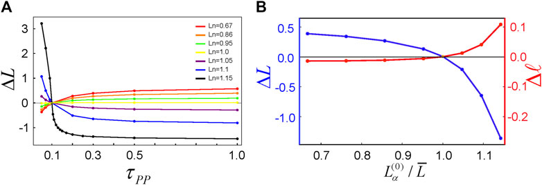
FIGURE 2. (A) The length difference ($\Delta L$) of the compartment boundary between the initial and final states of the sheet as a function of ${\tau }_{PP}$ and $L_n$. The quantity $L_n$ is given by $L_{\alpha }^{\left(0\right)}/\overline{L}$. The quantity $\overline{L}$ (=5.56) is the mean perimeter length of P cells in the initial state. (B) Plots of $\Delta L$ and the mean length difference ($\Delta \ell$) of cell boundaries between P cells as a function of $L_{\alpha }^{\left(0\right)}/\overline{L}$. In this simulation, ${\tau }_{PP}$ was changed from ${\tau }_{PP}=0.1$ (default) to ${\tau }_{PP}=0.3$ at t=0. The parameter values used here are the same as in Figure 1, except for the values of the parameters ${\tau }_{PP}$ and $L_{\alpha }^{\left(0\right)}$. In this simulation ${\tau }_{PP}$ is varied from 0.05 to 1.0, and $L_{\alpha }^{\left(0\right)}$ is varied from 4.4 to 7.6.

Here a question may arise. Why does the increase in ${\tau }_{PP}$ shorten the compartment boundary? In the case of an increase in ${\gamma }_{ij}$ at the compartment boundary, shortening of the compartment boundary is reasonable because the term in $U$ that contains ${\gamma }_{ij}$ (Eq. 1) makes shortening energetically preferable. However, in the case of a change in ${\tau }_{ij}$, this parameter represents the relaxation time defined in Eq. 3 and is not directly related to the potential energy $U$. Hence, it is not immediately apparent how ${\tau }_{PP}$ affects the length of the compartment boundary. To understand this, we first look at the data given in Figure 2B, where the quantity $\Delta \ell$ is the average length change of cell boundaries between P cells that contact the compartment boundary. These data indicate that, with the increase in ${\tau }_{PP}$, the cell boundaries between P cells became longer ($\Delta \ell$ increases), while the cell boundaries between A and P cells became shorter ($\Delta L$ decreases). This result suggests that, if we consider in this model a cell having cell boundaries with different relaxation times ${\tau }_{ij}$, the cell boundary having a large ${\tau }_{ij}$ would lengthen, while the cell boundary having a small ${\tau }_{ij}$ would shorten. To illustrate this property of the model, in the next subsection we conduct a simple analysis concerning the cell boundary length of a simple cell.

A Simple Analysis to Understand Why the New Vertex Model Lengthens the Cell Boundary with Large ${\tau }_{ij}$

Let us consider a single cell whose dynamics obey Eqs. 1–4 and whose shape is kept rectangular, in which the state of the cell is specified only by the quantities characterizing the vertical and horizontal boundaries of the cell. Let us denote the lengths of vertical and horizontal boundaries of the cell by ${\ell }_1$ and ${\ell }_2$, respectively. All the boundaries of the cell have the same contraction force $\gamma$ (>0), while the vertical and horizontal cell boundary have different relaxation times, ${\tau }_1$ and ${\tau }_2$, respectively. We are concerned with the cell’s steady state under these conditions. The potential function $U$ of this cell is given by

$U=\frac{K}{2}{\left({\ell }_1{\ell }_2-A^{\left(0\right)}\right)}^2+2\gamma \left({\ell }_1+{\ell }_2\right)+k\left[{\left({\ell }_1-{\ell }_1^{\left(M\right)}\right)}^2+{\left({\ell }_2-{\ell }_2^{\left(M\right)}\right)}^2\right].(5)$

The force balance equations at each boundary are given by $\partial U/\partial {\ell }_1=\partial U/\partial {\ell }_2=0$, which gives

$\begin{array}{l}\frac{1}{2}{\ell }_{2}K\left({\ell }_1{\ell }_2-A^{\left(0\right)}\right)+\gamma +k\left({\ell }_1-{\ell }_1^{\left(M\right)}\right)=0\\ \frac{1}{2}{\ell }_{1}K\left({\ell }_1{\ell }_2-A^{\left(0\right)}\right)+\gamma +k\left({\ell }_2-{\ell }_2^{\left(M\right)}\right)=0.\end{array}(6)$

In our model, ${\ell }_1$, ${\ell }_2$, ${\ell }_1^{\left(M\right)}$, and ${\ell }_2^{\left(M\right)}$ are independent variables, so ${\ell }_1^{\left(M\right)}$ and ${\ell }_2^{\left(M\right)}$ are not differentiated with ${\ell }_1$ and ${\ell }_2$. The time evolution equations for ${\ell }_1^{\left(M\right)}$ and ${\ell }_2^{\left(M\right)}$ are given by

$\begin{array}{l}\frac{d{\ell }_1^{\left(M\right)}}{dt}=-\frac{1}{{\tau }_1}\left({\ell }_1^{\left(M\right)}-{\ell }_1\right)-\frac{1}{2}\frac{\partial M}{\partial {\ell }_1^{\left(M\right)}}\\ \frac{d{\ell }_2^{\left(M\right)}}{dt}=-\frac{1}{{\tau }_2}\left({\ell }_2^{\left(M\right)}-{\ell }_2\right)-\frac{1}{2}\frac{\partial M}{\partial {\ell }_1^{\left(M\right)}},\end{array}(7)$

where ${\ell }_1^{\left(M\right)}$ and ${\ell }_2^{\left(M\right)}$ are the respective rest lengths of the vertical and horizontal cell boundaries, and $M$ is given by $M=\frac{k_{pm}}{2}{\left(2\left({\ell }_1^{\left(M\right)}+{\ell }_2^{\left(M\right)}\right)-L^{\left(0\right)}\right)}^2$, where $L^{\left(0\right)}$ is the preferred total resting length of this cell. The factor 1/2 in front of $\partial M/\partial {\ell }_i^{\left(M\right)}$ comes from the setup that the shape of this cell is rectangular, where both sides of the cell have the same quantities. To consider the steady state of this cell, we put $d{\ell }_i^{\left(M\right)}/dt=0$ in Eq. 7, to obtain

$\begin{array}{l}-\frac{1}{{\tau }_1}\left({\ell }_1^{\left(M\right)}-{\ell }_1\right)-k_{pm}\left(2\left({\ell }_1^{\left(M\right)}+{\ell }_2^{\left(M\right)}\right)-L^{\left(0\right)}\right)=0\\ -\frac{1}{{\tau }_2}\left({\ell }_2^{\left(M\right)}-{\ell }_2\right)-k_{pm}\left(2\left({\ell }_1^{\left(M\right)}+{\ell }_2^{\left(M\right)}\right)-L^{\left(0\right)}\right)=0.\end{array}(8)$

Although we can analytically solve Eqs. 6, 8 for the variables, ${\ell }_1,{\ell }_2,{\ell }_1^{\left(M\right)},{\ell }_2^{\left(M\right)}$, the forms of the solution are too complex to extract information about the ${\tau }_i$-dependence of ${\ell }_i$. Thus, we shall take another approach for this aim. First, we note that the terms $K\left({\ell }_1{\ell }_2-A^{\left(0\right)}\right)/2$ and $k_{pm}\left(2\left({\ell }_1^{\left(M\right)}+{\ell }_2^{\left(M\right)}\right)-L^{\left(0\right)}\right)$ are common to Eqs. 6, 8. Thus, we assign $p=K\left(A^{\left(0\right)}-{\ell }_1{\ell }_2\right)/2$ and $f=k_{pm}\left(L^{\left(0\right)}-2\left({\ell }_1^{\left(M\right)}+{\ell }_2^{\left(M\right)}\right)\right)$ and rearrange Eqs. 6, 8 to obtain ${\ell }_1=\frac{\gamma -{\tau }_{2}kf}{p}$ and ${\ell }_2=\frac{\gamma -{\tau }_{1}kf}{p}$. Subtracting ${\ell }_2$ from ${\ell }_1$ gives

${\ell }_1-{\ell }_2=\frac{kf}{p}({\tau }_1-{\tau }_2).(9)$

It should be noted here that $p$ is the pressure acting on the cell boundaries, and $p$ is positive when $\gamma >0$ because contraction forces acting on the cell boundaries tend to shrink these boundaries as well as the area of the cell, ${\ell }_1{\ell }_2$, such that ${\ell }_1{\ell }_2<A^{\left(0\right)}$. In addition, if $L^{\left(0\right)}$ is so large that $L^{\left(0\right)}>2\left({\ell }_1^{\left(M\right)}+{\ell }_2^{\left(M\right)}\right)$ is the case, $f$ becomes positive. In this case, the magnitude relationship between ${\ell }_i$ and ${\tau }_i$ is the same, i.e., when ${\tau }_1>{\tau }_2$, ${\ell }_1>{\ell }_2$, or vice versa (see Eq. 9). On the other hand, in the case where $L^{\left(0\right)}$ is small enough that $L^{\left(0\right)}<2\left({\ell }_1^{\left(M\right)}+{\ell }_2^{\left(M\right)}\right)$, the magnitude relationship between ${\ell }_i$ and ${\tau }_i$ becomes opposite, i.e., when ${\tau }_1>{\tau }_2$, ${\ell }_1<{\ell }_2$, and vice versa. This consideration suggests that there exists a characteristic value of $L^{\left(0\right)}$, denoted by $L^{\left(0\right)\ast }$, at which $f$ becomes zero. Indeed, such a value of $L^{\left(0\right)\ast }$ does exist, which is confirmed analytically. This property of the model appears in Figures 2A,B: when $L_{\alpha }^{\left(0\right)}>L^{\left(0\right)\ast }$, the compartment boundary is shortened and straightened, with a large ${\tau }_{ij}$, and vice versa. That is, P cells in contact with the compartment boundary have different relaxation times, ${\tau }_{PP}$ and ${\tau }_{AP}$, depending on the side (remembering that the compartment boundary is the boundary between A and P cells). Since we have set ${\tau }_{PP}>{\tau }_{AP}$ and $L_{\alpha }^{\left(0\right)}>L^{\left(0\right)\ast }$, the cell boundary between P cells lengthens, and the cell boundary between A and P cells shortens (Figure 1C).

While the above analysis is restricted to a case in which the cell shape is rectangular, the relation between ${\ell }_i$ and ${\tau }_i$ continues to hold when the cell shape is pentagonal, hexagonal, etc. (see Supplementary Appendix 2). In addition, although the preceding analysis concerned the case of a single cell, a similar relation between ${\ell }_i$ and ${\tau }_i$ continues to apply in the case of a cell sheet, i.e., when the cell boundary has a longer relaxation time, the cell boundary length tends to become longer.

Application 2: The Response of the Cell Sheet When Stretched by External Forces

In this section, we consider the stretch of a cell sheet by external forces. In the previous vertex models, when the cell sheet is stretched greatly enough by external forces, the sheet necessarily undergoes cell remodeling (Figures 3A,B; Supplementary Movie 3; the formulation of the previous vertex model is given in Supplementary Appendix 1). This behavior originates in two properties of the previous vertex model: 1) cell shape tends to be round, due to the quadratic term ($\frac{K_p}{2}{\displaystyle \sum _{\mathrm{cell}\alpha }{\left(L_{\alpha }-L_0\right)}^2}$) in U, and 2) there is no repulsive force between vertices to prevent rounding of the cell. We will explain property 2) in more detail. Consider the case where external forces deform the cell shape well away from the preferred round shape, i.e., an elliptical shape with a large ratio of width to height. In this situation, the cell shape tends to return to roundness due to property 1). As a result, cell remodeling occurs (see Supplementary Movie 3). To put it another way, the previous vertex model has no repulsive force between vertices to maintain the cell in an elliptical shape. The present vertex model, on the other hand, has a repulsive force on the cell boundary when $1/{\tau }_{ij}=0$ as indicated below. This is the meaning of statement 2). Moreover, experimental results show that even when the cell sheet is stretched greatly enough by external forces, remodeling of the cell configuration does not necessarily occur [17]. The discrepancy between the numerical and experimental results implies the necessity to improve the previous vertex model. In our modified vertex model, in fact, cell remodeling does not necessarily occur when the cell sheet is stretched (Figure 3C; Supplementary Movie 4), but whether or not remodeling occurs depends upon the parameters of the model. If ${\tau }_{ij}$ in Eq. 3 is infinitely large, i.e., $1/{\tau }_{ij}$ is zero, the time evolution equation for ${\ell }_{ij}^{\left(M\right)}$ is decoupled from ${\ell }_{ij}$, and the value of ${\ell }_{ij}^{\left(M\right)}$ is determined by the initial values of ${\ell }_{ij}^{\left(M\right)}$ and $L_{\alpha }^{\left(0\right)}$. That is, ${\ell }_{ij}^{\left(M\right)}$ becomes a constant independent of ${\ell }_{ij}$. In this case, the third term in Eq. 1 generates a repulsive force between vertices, and the elliptical shape is retained even in the steady state. On the other hand, if the value of ${\tau }_{ij}$ is finite, ${\ell }_{ij}^{\left(M\right)}$ tends to follow ${\ell }_{ij}$ according to Eq. 3, and repulsive forces coming from the third terms are weakened. Then, the cells eventually undergo remodeling, and each cell becomes round (Figure 3D and Supplementary Movie 2). The final cell configuration in the new vertex model for finite ${\tau }_{ij}$ is not necessarily the same as that in the former vertex model because the order of cell remodeling affects the final state (see Supplementary Movies 3, 5). The speed at which the system approaches the energetically minimum state depends on the value of ${\tau }_{ij}$; the larger ${\tau }_{ij}$ is, the slower this approach. Thus, ${\tau }_{ij}$ plays a role analogous to a friction coefficient for the relative movement between the ith and jth vertices.

FIGURE 3

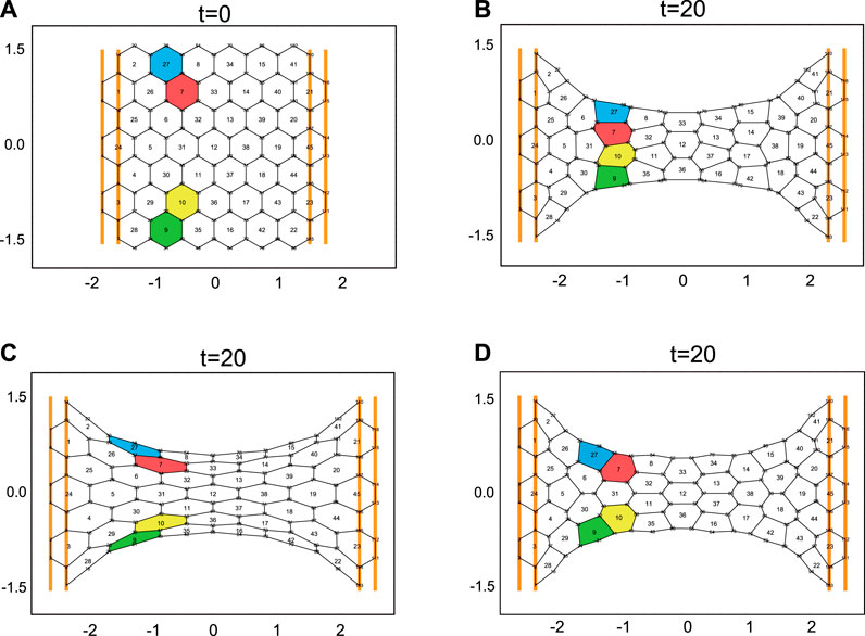
FIGURE 3. (A) The initial configuration of the cell sheet. At time t = 0, the cell sheet begins to be stretched by external forces, which are represented by the orange bars. At these bars, the cell boundaries are fixed, and the bars are shifted with time (for the movement of the bars see Supplementary Movies 3–5). (B) The final cell configuration of the sheet stretched by external forces. The cell sheet dynamics are implemented by the previous vertex model (see Supplementary Appendix 1). The time evolution equation for $r_i$ is given by ${\dot{r}}_i=-\left(\left(1/\widehat{\eta }\right)\right)\partial U/\partial r_i$, where $\widehat{\eta }$ is a constant. The parameter values used here are $K=1$, $A_{\alpha }^{\left(0\right)}=0.22$, ${\widehat{\gamma }}_{ij}=1.0$. $\widehat{\eta }=1.0$, $L_0=1.65$, and $K_p=50$. (C) The final cell configuration of the sheet stretched by the external forces. The cell sheet dynamics are implemented by the present vertex model. The parameter values used here are $K=1$, $A_{\alpha }^{\left(0\right)}=0.22$,${\gamma }_{ij}=1.0$, $\eta =0.01$, $L_{\alpha }^{\left(0\right)}=1.65$, $k_{pm}=50$, $k=100$, and$1/{\tau }_{ij}=0$. (D) The final cell configuration of the sheet after being stretched by external forces using the present vertex model with finite ${\tau }_{ij}=0.1$. The other parameter values are the same as those in (C).

Conclusion and Discussion

In this paper, we provided a novel formulation of the vertex model that separately treats the contraction force on the cell boundary and the strength of adhesion between cells, by considering the resting length of the cell boundary and its dynamics. We applied this vertex model to understanding the straightening of the compartment boundary observed in the fruit fly pupa and showed that the model recaptures compartment boundary straightening in response to an increase in strength of adhesion between P cells. We also used this model to examine the stretching of a cell sheet by external forces and gained insights into cell remodeling resulting from the stretch. This model has the potential to clarify points that were ambiguous in the previous vertex model. One such point is the frictional force exerted on the vertex. In the previous model, the equation for time evolution of vertex positions is obtained by assuming that total mechanical force on the vertex and frictional force on the vertex are balanced. However, the meaning and origin of the frictional force on the vertex had not yet been well discussed. The present vertex model has the potential to explain the origin and meaning of the frictional force between vertices. Indeed, as mentioned in Application 2: The Response of the Cell Sheet When Stretched by External Forces, changes in ${\tau }_{ij}$in Eq. 3 change the speed of cell remodeling, and the meaning of ${\tau }_{ij}$is interpreted through Eq. 3. This model could be applicable to the phenomenon [18] where E-cadherin binding protein (p120-catenin) speeds cell intercalation.

Recently, it has been reported that cell intercalation (cell remodeling) in the cell sheet is related to endocytosis at the cell boundary of epithelial cells [12, 14]. In our model, the effect of endocytosis frequency at the cell boundary is represented by ${\tau }_{ij}$ in Eq. 3. The present vertex model can be applied to the phenomenon [12] where blocking endocytosis at the cell boundary inhibits cell remodeling. Relaxation time ${\tau }_{ij}$ in Eq. 3 can be changed when expression levels of molecules associated with endocytosis, such as clathrin, dynamin, and its ortholog, change.

As demonstrated in Figure 3C, the cell sheet described by the present vertex model does not necessarily undergo cell intercalation even when the cells are largely deformed by external forces. Similar behaviors of epithelia are sometimes observed in experiments. A representative example of this is the defect in the formation of the tracheal system in the fruit fly embryo [19]. In the control case of the tracheal system, the tube consisting of epithelial cells undergoes cell intercalation and elongates along the long axis of the tube, during which the tip cells of the tube keep pulling the stalk cells toward the direction of the tip cells. The pulling forces of the tip cells were considered to a dominant factor for cell intercalation in the tube. However, expression of some molecules (e.g., Spalt) inhibits cell intercalation, and tube elongation stops at a certain length, even though the tip cells continue to pull the stalk cells [19]. This experimental result implies that for cell intercalation proceeding external forces on the cell sheet are not sufficient and other factors are necessary. We might be able to consider the factors necessary for cell intercalation through the notion of ${\tau }_{ij}$ in Eq. 3. As we stated above, molecules that change the turnover rate of cell membrane can change the value of ${\tau }_{ij}$. It is considered that ${\tau }_{ij}$ closely relates to the strength of adhesion between cell membranes and the turnover rate of the adhesion molecules, which may be checked with the present vertex model and experimental results.

In the morphological study of multicellular organisms, it becomes more important to investigate responses of the cell sheet to external mechanical perturbations [17]; thus, more detailed research on this issue using cell-based mathematical models, such as vertex models, is expected.

Data Availability Statement

The original contributions presented in the study are included in the article/Supplementary Material, further inquiries can be directed to the corresponding author.

Author Contributions

KS and DU designed the concept of the paper. KS created the model, and performed its numerical simulations and analyses. KS and DU wrote the paper. KS and DU contributed to the review and approval of the paper for publication.

Funding

This work was supported by Global Station for Soft Matter at Hokkaido University (KS), the Cooperative Research Program of “NJRC Mater. and Dev.” (KS), and MEXT/JSPS KAKENHI Grant Nos. 17H02939 (KS and DU), 20K03871 (KS), 18H01135 (KS), 17K07402 (DU), and 21K06144 (DU).

Conflict of Interest

The authors declare that the research was conducted in the absence of any commercial or financial relationships that could be construed as a potential conflict of interest.

Acknowledgments

We would like to thank Y. Ishimoto, M. Nishikawa, T. Shibata, E. Kuranaga, S. Okuda, T. Taguchi, and S. Hayashi for valuable comments and discussions.

Supplementary Material

The Supplementary Material for this article can be found online at: https://www.frontiersin.org/articles/10.3389/fphy.2021.704878/full#supplementary-material

References

1. Friedl P, Gilmour D. Collective Cell Migration in Morphogenesis, Regeneration and Cancer. Nat Rev Mol Cel BiolJul (2009) 10(7):445–57. doi:10.1038/nrm2720

CrossRef Full Text | Google Scholar

2. Fletcher AG, Osterfield M, Baker RE, Shvartsman SY. Vertex Models of Epithelial Morphogenesis. Biophysical J (2014) 106(11):2291–304. doi:10.1016/j.bpj.2013.11.4498

CrossRef Full Text | Google Scholar

3. Alt S, Ganguly P, Salbreux G. Vertex Models: from Cell Mechanics to Tissue Morphogenesis. Phil Trans R Soc B (2017) 372(1720):20150520. doi:10.1098/rstb.2015.0520

PubMed Abstract | CrossRef Full Text | Google Scholar

4. Rauzi M, Verant P, Lecuit T, Lenne P-F. Nature and Anisotropy of Cortical Forces Orienting Drosophila Tissue Morphogenesis. Nat Cel Biol. (2008) 10:1401–10. doi:10.1038/ncb1798

CrossRef Full Text | Google Scholar

5. Hočevar Brezavšček A, Rauzi M, Leptin M, Ziherl P. A Model of Epithelial Invagination Driven by Collective Mechanics of Identical Cells. Biophys J (2012) 103(5):1069–77. doi:10.1016/j.bpj.2012.07.018

PubMed Abstract | CrossRef Full Text | Google Scholar

6. Okuda S, Inoue Y, Watanabe T, Adachi T. Coupling Intercellular Molecular Signalling with Multicellular Deformation for Simulating Three-Dimensional Tissue Morphogenesis. Interf Focus. (2015) 5:20140095. doi:10.1098/rsfs.2014.0095

PubMed Abstract | CrossRef Full Text | Google Scholar

7. Sato K, Hiraiwa T, Shibata T. Cell Chirality Induces Collective Cell Migration in Epithelial Sheets. Phys Rev Lett (2015) 115:188102. doi:10.1103/physrevlett.115.188102

PubMed Abstract | CrossRef Full Text | Google Scholar

8. Nagai T, Honda H. A Dynamic Cell Model for the Formation of Epithelial Tissues. Philosophical Mag B (2001) 81:699–719. doi:10.1080/13642810108205772

CrossRef Full Text | Google Scholar

9. Farhadifar R, Röper J-C, Aigouy B, Eaton S, Jülicher F. The Influence of Cell Mechanics, Cell-Cell Interactions, and Proliferation on Epithelial Packing. Curr Biol (2007) 17:2095–104. doi:10.1016/j.cub.2007.11.049

PubMed Abstract | CrossRef Full Text | Google Scholar

10. Landsberg KP, Farhadifar R, Ranft J, Umetsu D, Widmann TJ, Bittig T, et al. Increased Cell Bond Tension Governs Cell Sorting at the Drosophila Anteroposterior Compartment Boundary. Curr Biol (2009) 19:1950–5. doi:10.1016/j.cub.2009.10.021

PubMed Abstract | CrossRef Full Text | Google Scholar

11. Iijima N, Sato K, Kuranaga E, Umetsu D. Differential Cell Adhesion Implemented by Drosophila Toll Corrects Local Distortions of the Anterior-Posterior Compartment Boundary. Nat Commun (2020) 11(1):6320. doi:10.1038/s41467-020-20118-y

PubMed Abstract | CrossRef Full Text | Google Scholar

12. Blackie L, Tozluoglu M, Trylinski M, Walther RF, Schweisguth F, Mao Y, et al. A Combination of Notch Signaling, Preferential Adhesion and Endocytosis Induces a Slow Mode of Cell Intercalation in the Drosophila Retina. Development 148. (2021). p. 197301. doi:10.1242/dev.197301

CrossRef Full Text | Google Scholar

13. Kaplan J, Moskowitz M. Studies on the Turnover of Plasma Membranes in Cultured Mammalian Cells. Biochim Biophys Acta (Bba) - Biomembranes (1975) 389(2):306–13. doi:10.1016/0005-2736(75)90323-5

CrossRef Full Text | Google Scholar

14. Levayer R, Pelissier-Monier A, Lecuit T. Spatial Regulation of Dia and Myosin-II by RhoGEF2 Controls Initiation of E-Cadherin Endocytosis during Epithelial Morphogenesis. Nat Cel Biol (2011) 13(5):529–40. doi:10.1038/ncb2224May

PubMed Abstract | CrossRef Full Text | Google Scholar

15. Umetsu D, Dahmann C. Compartment Boundaries. Fly (2010) 4(3):241–5. doi:10.4161/fly.4.3.12173

PubMed Abstract | CrossRef Full Text | Google Scholar

16. Liang X, Michael M, Gomez G. Measurement of Mechanical Tension at Cell-Cell Junctions Using Two-Photon Laser Ablation. Bio-protocol (2016) 6(24):e2068. doi:10.21769/BioProtoc.2068

PubMed Abstract | CrossRef Full Text | Google Scholar

17. Duda M, Kirkland NJ, Khalilgharibi N, Tozluoglu M, Yuen AC, Carpi N, et al. Polarization of Myosin II Refines Tissue Material Properties to Buffer Mechanical Stress. Dev Cel (2019) 48(2):245–60. doi:10.1016/j.devcel.2018.12.020

PubMed Abstract | CrossRef Full Text | Google Scholar

18. Iyer KV, Piscitello-Gómez R, Paijmans J, Jülicher F, Eaton S. Epithelial Viscoelasticity Is Regulated by Mechanosensitive E-Cadherin Turnover. Curr Biol (2019) 29(4):578–91. doi:10.1016/j.cub.2019.01.021

PubMed Abstract | CrossRef Full Text | Google Scholar

19. Ribeiro C, Neumann M, Affolter M. Genetic Control of Cell Intercalation during Tracheal Morphogenesis in Drosophila. Curr Biol (2004) 14(24):2197–207. doi:10.1016/j.cub.2004.11.056.11

PubMed Abstract | CrossRef Full Text | Google Scholar