Criterion for Imminent Failure During Loading—Discrete Element Method Analysis

It has recently been reported that the equal load sharing fiber bundle model predicts the rate of change of the elastic energy stored in the bundle reaches its maximum before catastrophic failure occurs, making it a possible predictor for imminent collapse. The equal load sharing fiber bundle model does not contain central mechanisms that often play an important role in failure processes, such as localization. Thus, there is an obvious question whether a similar phenomenon is observed in more realistic systems. We address this question using the discrete element method to simulate breaking of a thin tissue subjected to a stretching load. Our simulations confirm that for a class of virtual materials which respond to stretching with a well-pronounced peak in force, its derivative and elastic energy we always observe an existence of the maximum of the elastic energy change rate prior to maximum loading force. Moreover, we find that the amount of energy released at failure is related to the maximum of the elastic energy absorption rate.

1. Introduction

Fracturing, breaking, or more generally fragmentation of solid materials is a common physical processes that we meet in our daily lives. At the same time, it is one of the most complex processes covering a huge range of length and energy scales from atomic scale (breaking of chemical bonds) up to earthquakes (kilometer scale). This, together with a huge diversity of materials composition and variety of loading conditions leads to the aforementioned complexity. On the other hand, the fracture processes are extremely important for both industry and society. There is thus no surprise that a huge effort has been made to understand the fracture process in order to use it efficiently in controlled conditions (industry) and to prevent catastrophic failures (engineering, earthquakes). Furthermore, breaking/fracture dynamics plays central role in geophysical phenomena, such as snow avalanches [1], landslides [2, 3] as well as in stretching in biological materials [4]. The study of the breaking process has recently led to a discovery of a robust phenomenon which occurs before catastrophic failure (collapse) of composite materials under stress [5]. It has been found that the simple Fiber Bundle Model (FBM), a representative of fibrous materials, predicts existence of a maximum of the elastic energy absorption rate prior to a catastrophic failure point, namely the strain value at which the fiber bundle sustains the largest loading (stretching) force. Although the FBM has been proved to be a very powerful theoretical tool [6] it is based on some simplifications with respect to realistic processes. The obvious question thus arises if similar phenomena can also be predicted by other methods capable of grasping more realistic breaking scenarios. To answer this question, we have turned our attention toward numerical simulations of the breaking process by means of the Discrete Element Method (DEM) [7]. The two methods, FBM and DEM, we are dealing with in this paper, represent two complementary approaches to the study of fracture or breaking processes.

The Fiber Bundle Model [8] represents an approach which, through appropriate generalizations and simplifications, attempts to grasp the most important elements of fracturing process in composite materials. On the other hand, the numerical Discrete Element Method [7, 9] has the capability of describing more realistic failure processes using the principles of a classical dynamics. Both methods exhibit some similarities which make their conjecture an interesting and efficient way of transferring theoretical concepts to realistic physical scenarios. Let us briefly discuss this point. The basic feature of both methods is a discrete representation of the medium under investigation. The FBM represents it as a finite number of fibers joining two clamps stretching the medium [6]. In the DEM approach the medium is represented by an assemble of interacting and bonded particles subjected to an external loading. Upon this loading, the fibers in FBM and inter-particles bonds in DEM, bearing part of an external load, break according to assumed rules if the stretching force exceeds some threshold values. The threshold probability distribution of fibers strength and the model of inter-particle interactions fully and uniquely determine the dynamics of the system. In the current application we have further enhanced this similarity by choosing in DEM simulations a classical, elastic-brittle interaction model. It assumes that bonds joining near-neighborhood particles are represented by perfectly elastic “springs” which break if extended over some critical value, just like the fibers in the FBM model. The fibers and inter-particle bonds braking possibilities make both methods highly non-linear and capable of addressing problems with non-trivially evolving boundary conditions, like, for example, creating a free surface by fracturing.

The most obvious difference between the two methods is that fibers in FBM are clamped between two rigid bars, which is not the case in the DEM approach. The inter-particle bonds in DEM can be viewed as a “micro-fibers” joining only neighborhood particles. However, it is worth to mention that during a loading evolution a coherent behavior of these micro-fibers can lead to the creation of macroscopic “super-fibers” joining loading clamps, like fibers in the FBM. Moreover, if particles are randomly packed, the inter-particle bonds are randomly orientated in space, in contradiction to the FBM fibers which are always parallel to the external load. Comparing both approaches we would finally point out that DEM inherently includes geometry of the analyzed body, while FBM does not. At first sight, this seems to be in a favor of DEM but it also leads to some serious shortages of the method. The inclusion of geometrical aspects into fracture simulations mixes kinematic (e.g., acoustic wave propagation effects) and dynamical effects due to bond-breaking. It makes the inference about breaking process much more complex. On the other hand, this feature of DEM as well as the aforementioned similarities open up a possibility of transmitting concepts from the FBM abstraction level to the “real world.”

In this work we explore the possibility of verifying the appearance of the maximum of an elastic energy absorption rate prior to the catastrophic failure predicted by the FBM [5] is also visible in DEM simulations. To answer this question, we have designed a series of numerical simulations of stretching a thin tissue. The limitation to such a quasi-two-dimensional case (often referred to as a 2.5D problem) is fully intentional. On one hand, we want to avoid possible complications introduced by a fully 3D approach, but on the other hand we wish to allow for a full development of local inter-particle interactions, which requires a full 3D neighborhood of each particle. The underlying concept of the theoretical analysis and numerical simulations is sketched in Figure 1, where the cartoon of stretched bundle of fibers and the stretched thin tissue built of spherical particles are shown. In the case of the FBM, stretched fibers break sequentially from the weakest to the strongest. In case of the DEM simulations, dragging up the upper horizontal edge of the tissue causes the breaking of inter-particle bonds and finally leads to its failure. For the sake of clarity, the most important parameters are graphically illustrated in Figure 2 using an example of DEM simulated loading curves, describing the evolution of dragging force, elastic energy and its derivative with extension of the sample.

FIGURE 1

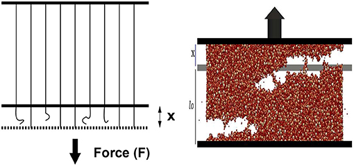
Figure 1. (Left) the fiber bundle model—parallel fibers are placed between two rigid bars and are stretched by an amount x by applying a force F at the lower bar. (Right) The discrete element model—a thin tissue built of interconnected spherical particles vertically stretched using a constant velocity. The initial length of the fibers (left) and the initial height of the tissue are also shown.

FIGURE 2

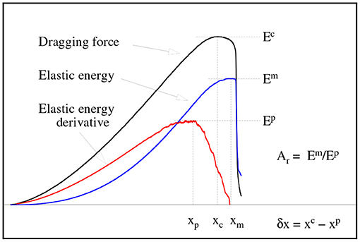
Figure 2. Illustration of parameters used in the analysis. In the case of the DEM analysis, the vertical deformation (strain) parameters, x, x_c, and x_p, are scaled by the initial height l₀ of the tissue.

Answering the posed question goes through the following steps: After the Introduction (section 1) we give a short background of the studies on breaking of FBM in section 2. In several subsections of section 2 we discuss strength and stability in FBM, energy variations during breaking process and the prediction concerning the existence of a “precursor” of the collapse point. In the next section (section 3) the DEM method is shortly presented, followed by a detailed description of performed numerical simulations in section 4. The simulation results are discussed in section 5, and we give some final remarks and conclusions in section 6.

2. Fiber Bundle Model

When we stretch a system, composed of elements with different strength thresholds, weaker elements fail first. As the surviving elements have to support the force, stress (force per element) increases and that can trigger more element-failure. With continuous stretching, at some point the system collapses completely.

There are several physics-based models [10–12] that can describe such a scenario. The FBM is one of those models being a useful tool for studying fracture and failure [6, 13, 14] of composite materials under different stretching conditions. In 1926, Peirce introduced the Fiber Bundle Model [8] to study the strength of cotton yarns in connection with textile engineering. Some static behavior of such a bundle was discussed by Daniels in 1945 [13] and the model was brought to the attention of physicists in 1989 by Sornette [15], who then proceeded mainly to explore the failure dynamics and avalanche phenomena in this model [16–18].

The simplicity of the model allows one to achieve analytic solutions [14, 19] to an extent that is not possible in any of the other fracture model. For these reasons, FBM is widely used as a model of fracture-failure that extends beyond disordered solids.

In the FBM (Figure 1), a large number of parallel Hookean springs or fibers are clamped between two horizontal clamps; the upper one (fixed) helps hanging the bundle while the load hangs from the lower one. The springs or fibers are assumed to have different breaking strengths. Once the load per fiber exceeds a fiber's threshold, it fails and can not carry load any more. The load/stress it carried is now transferred to the surviving fibers. If the lower platform deforms under loading, fibers closer to the just-failed fiber will absorb more of the load compared to those further away. Examples of such models are the Soft Clamp FBM [20] or the one proposed by Hidalgo et al.[21]. The extreme version of such models is the Local Load Sharing FBM [22] where the forces carried by the failed fiber is absrobed by its sucrviving neighbors. If the lower clamp is rigid, the load is equally distributed to all the surviving fibers. This is the Equal Load Sharing (ELS) FBM.

We will in the following only discuss the ELS FBM, which we refer to as the FBM in the following.

2.1. Strength and Stability of the Fiber Bundle Model

Let us consider a fiber bundle model having N parallel fibers. Each fiber responds linearly with a force f to the stretch value x as f = κx, where κ is the spring constant. If the stretch x exceeds the strength threshold, the fiber fails irreversibly.

The strength thresholds of the fibers are drawn from a probability density p(x) described by the corresponding cumulative probability P(x). For example, for the uniform distribution on the unit interval we have

$\begin{array}{ll}p(x)=1;P(x)=x.& (1)\end{array}$

If N_f fibers have failed at a stretch x, then the bundle carries a force

$\begin{array}{ll}F=(N-N_f)\kappa x=N(1-P(x))\kappa x& (2)\end{array}$

which for the uniform distribution is a parabola as shown in Figure 3.

FIGURE 3

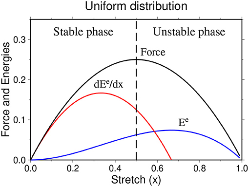
Figure 3. Force (black curve), elastic energy (blue curve), and elastic energy change rate (red curve) against the stretch x for uniform distribution of the fiber strengths in the bundle.

The force-maximum is the strength of the bundle and the corresponding stretch value x_c is the critical stretch beyond which the bundle collapses. Therefore, there are two distinct phases of the system: stable phase for 0 < x ≤ x_c and unstable phase for x > x_c. The critical stretch value is found by setting dF(x)/dx = 0:

$\begin{array}{ll}1-x_{c}p(x_c)-P(x_c)=0.& (3)\end{array}$

and the solution for the uniform threshold distribution reads

$\begin{array}{ll}{x}_c=\frac{1}{2}.& (4)\end{array}$

In a similar way, one may calculate the critical strength of the bundle by putting x_c value in the force expression (Equation 2).

$\begin{array}{ll}\frac{F_c}{N}=\frac{1}{4}.& (5)\end{array}$

2.2. Energy Variation and Warning Sign of Collapse

Work of an external load stretching the bundle converts into elastic energy of the fibers E^e and is partially released as damage energy E^d of broken fibers. When N is large, one can express E^e and E^d in terms of the stretch x as [5]

$\begin{array}{ll}{\text{E}}^e(x)=\frac{N\kappa }{2}{x}^2(1-P(x)),& (6)\end{array}$

and

$\begin{array}{ll}{\text{E}}^d(x)=\frac{N\kappa }{2}{\displaystyle {\int }_0^x}dy\left[p(y)y^2\right].& (7)\end{array}$

For the uniform distribution within the range (0, 1), the Equations (6, 7) reads

$\begin{array}{ll}{\text{E}}^e(x)=\frac{N\kappa }{2}{x}^2(1-x),& (8)\end{array}$

and

$\begin{array}{ll}{\text{E}}^d(x)=\frac{N\kappa }{6}{x}^3.& (9)\end{array}$

Clearly, the damage energy increases steadily with the stretch, but elastic energy has a maximum. Setting dE^e(x)/dx = 0, one gets the condition for the position of the elastic energy maximum

$\begin{array}{ll}2(1-P(x_m))-x_{m}p(x_m)=0,& (10)\end{array}$

whose solution for the uniform distribution reads [5].

$\begin{array}{ll}{x}_m=2/3=4/3x_c.& (11)\end{array}$

Although the elastic energy has a maximum, it appears after the critical extension value, i.e., in the unstable phase of the system. Therefore, it can not help us to predict the catastrophic failure point of the system.

The situation is different if we consider the rate of elastic energy change ${E}(x)=d{\text{E}}^e(x)/dx$ which reads [5]

$\begin{array}{ll}{E}(x)=\frac{N\kappa }{2}\left[2x(1-P(x))-x^{2}p(x)\right].& (12)\end{array}$

Now, one can demonstrate that ${E}(x)$ has a maximum and, this maximum appears before the critical extension value x_c (Figure 3). Indeed, one can calculate the value of stretch x = x_p at which ${E}$ has a maximum.

Taking derivative of $d{E}/dx$,

$\begin{array}{ll}\frac{d{E}(x)}{dx}=\frac{N\kappa }{2}\left[2(1-P(x))-4xp(x)-x^2{p}^{\prime }(x)\right];& (13)\end{array}$

where p′(x) stands for derivative of p(x). Setting $d{E}(x)/dx=0$ at x = x_p we get the following solution for the uniform distribution

$\begin{array}{ll}{x}_p=\frac{2}{3}{x}_c.& (14)\end{array}$

Thus, the rate of change of elastic energy shows a maximum before the actual failure appears. This result has been proven under weak conditions and demonstrated also for other probability distributions [5]. The obvious question at this moment is what information about upcoming failure this “precursor” provide us with. To answer this question, let us reformulate the problem at hand in the following way.

Let us assume that we know that maximum of the elastic energy absorption rate occurs at given x_p and let us assume that its value at x_p is ${{E}}_{max}$. Knowing these two values can we predict quantitatively a failure time (measured in units of x) and can we predict its size in term of the released elastic energy? The answer can be obtained from equations describing the dependences of E^e and ${E}$ on x as well as conditions for their maxima. The relations between x_c, x_m and x_p for a general power law distribution

$\begin{array}{ll}\begin{array}{c}p(x)=(1+\alpha )x^{\alpha },\hfill \\ P(x)=x^{1+\alpha },\hfill \end{array}& (15)\end{array}$

where α > 0 and 0 ≤ x ≤ 1 reads

$\begin{array}{ll}\begin{array}{c}{x}_c={\left(\frac{3+\alpha }{2}\right)}^{\frac{1}{1+\alpha }}{x}_p\hfill \\ x_m={(2+\alpha )}^{\frac{1}{1+\alpha }}{x}_p\hfill \end{array}& (16)\end{array}$

For the purpose of later comparison with DEM simulations, we introduce another parameter, δ_x, describing the delay of the critical value with respect to x_p: δ_x = x_c − x_p, and the coefficient Γ quantifying a retardation of the point when elastic energy reaches maximum x_m with respect to x_c:

$\begin{array}{ll}{x}_m=x_c+\Gamma {\delta }_x,& (17)\end{array}$

in terms of the δ_x scale.

For the power law distribution, the explicit form for δ_x anf Γ reads

$\begin{array}{ll}{\delta }_x=\left[{\left(\frac{3+\alpha }{2}\right)}^{\frac{1}{1+\alpha }}-1\right]x_p,& (18)\end{array}$

and

$\begin{array}{ll}\Gamma =\frac{{\left(2+\alpha \right)}^{\frac{1}{1+\alpha }}-{\left(\frac{3+\alpha }{2}\right)}^{\frac{1}{1+\alpha }}}{{\left(\frac{3+\alpha }{2}\right)}^{\frac{1}{1+\alpha }}-1}.& (19)\end{array}$

Both δ_x and Γ are monotonically decreasing functions of α and reach their maxima for the uniform distribution: δ_x(α = 0) = 1/6 and Γ(α = 0) = 1, which means that in this case x_p and x_m are symmetrically located with respect to x_c.

Next, let us define yet another quantity A^r which relates the maximum of elastic energy E^e(x) to the maximum of the energy absorption rate ${E}$(x).

$\begin{array}{ll}{A}^r=\frac{{\text{E}}_{max}^e}{x_p{{E}}_{max}}=\frac{{\text{E}}^e\left(x_m\right)}{x_p{E}\left(x_p\right)},& (20)\end{array}$

so

$\begin{array}{ll}{\text{E}}_{max}^e=A^r{x}_p{{E}}_{max}& (21)\end{array}$

The x_p factor assures not only the dimensionality of A^r but also leads to A^rindependent of x_p for power law distribution, as shown below. For a given probability distribution A^r reads

$\begin{array}{ll}{A}^r=\frac{1}{2}\frac{x_m^{3}p\left(x_m\right)}{3x_p^{3}p\left(x_p\right)+x_p^4{p}^{\prime }\left(x_p\right)}.& (22)\end{array}$

For the power law distribution (Equation 15) the explicit form of A^r can be easily found

$\begin{array}{ll}{A}^r=\frac{1}{2}\frac{{(2+\alpha )}^{\frac{3+\alpha }{1+\alpha }}}{3+\alpha }.& (23)\end{array}$

Let us note, that in this case A^r is constant, independent of x_p, and reaches its maximum value for uniform distribution A^r(α = 0) = 4/3.

Interpretation of Equations (16), (21), and (22) is quite simple. For the considered power law distribution, the pair of parameters (x_p, ${{E}}_{max}$) fully determines the upcoming failure, both a moment of its occurrence (x_c) as well as the amount of elastic energy (Eemax) which is released during the catastrophic failure.

3. Discrete Element Method

The Discrete Element Method (DEM) [7] is the numerical method originally developed for simulating the behavior of granular media. It represents a medium under consideration as an ensemble of geometrical, perfectly elastic objects (originally circles in 2D) that interact with each other by repulsive forces due to surface contacts. The original Cundal idea has been extended by incorporating more complex particle interaction schemes and, particularly, by introducing bonds between particles—internal forces [23, 24] joining particles in a single piece. This has changed the DEM method to the modern simulation technique situated between the molecular dynamics from one side and the fluid (continuum) mechanics from other side [9, 25, 26].

The most important feature of the DEM method is a mathematical representation of the medium by a set of interacting finite size particles whose dynamics directly follows from the Newton equations of motion. Such a direct approach has an obvious advantage. It does not use any continuity, conservation, or other assumptions typical for continuum mechanics. One of the most important consequences is that DEM is particularly suitable for solving problems with complex, non-trivially evolving boundary conditions. This is just the case of a fracturing process.

Finally, let us note that DEM is a particular numerical technique of solving general multi-body static or dynamic tasks. Thus, in the application discussed here it allows to simulate temporal evolution of objects prior to fracture nucleation similar to continuum mechanics, through a period of development of a micro-fracture system and dynamical breaking like fracture mechanics, and, finally, can also include post-failure dynamics. This last issue is very interesting because laboratory data cannot provide reliable information about just-after-failure situation, which, on the other hand, seems to be crucial for large scale (seismology) analysis and is also interesting from a theoretical point of view [24, 27].

There exists a number of implementations of the DEM method as ready-to-use software. Our choice for the analysis presented here is the Esys-Particle software developed at the University of Queensland, Australia [28, 29]. We have chosen this particular software for many reasons as discussed in Debski and Klejment [30]. A detailed description of the software can be found in Abe et al. [28].

The Esys-Particle software provides a number of inter-particle interaction models and methods of simulating external loads. In our analysis we have used the standard elastic-brittle interaction model [9, 24]. The most essential element of this model are elastic bonds joining pairs of neighborhood particles and representing Hookean attracting or repulsing central force if bonded particles change their relative distance:

$\begin{array}{ll}\overrightarrow{F}=-k_n{\delta }_r\frac{\overrightarrow{r}}{\left|\overrightarrow{r}\right|},& (24)\end{array}$

where $\overrightarrow{r}$ is a vector of relative position of particles, δ_r denotes a change of particle distance and kn is a strength of inter-particle interaction (“spring constant”). However, if a distance between the particles increases by more then a critical distance b_d, the bond breaks and disappears. If all bonds attached to a given particle break it becomes the “unbonded particle.” Summarizing, the used inter-particle interaction model is fully defined by a pair of parameters (k_n, b_d).

DEM simulates temporal evolution of a given system by an explicit time integration of equations of motion for all particles including external and inter-particle forces. At each time step positions and velocities of the particles and the acting forces are calculated and used to move the particles from the current to new positions. Then the time is increased by a predefined time step and procedure is repeated until a stopping criterion is met. Within the Esys-Particle software the Verlet integration schemata is used what assure conservation of system energy [28].

4. Numerical Experiment—Setup and Data Processing

Our DEM simulations deal with the simplest fracture dynamics task, namely the fracturing of materials under tensional load (mode 1 in the standard fracture mechanics classification). Taking into account the goal of the analysis, all performed simulations were conducted using the setup shown in Figure 1 with the following details.

Firstly, to avoid possible complications due to the full 3D analysis and speed up (lengthy) calculations we have considered only a 2.5D case—a thin tissue. Its size was assumed to be: depth D = 5 mm, height L = 25 mm, and width W = 80 mm. This numerical sample was built of spherical particles with radii in the range 0.2–0.6 mm distributed according to the log-normal distribution truncated to this range. Particles were randomly distributed in space, which we have achieved by means of the GenGeo algorithm [28]—a part of the Esys-Particle software. The sample consists altogether of almost 25,000 particles bonded by almost 125 thousand bonds. The same numerical sample was used in all simulations.

Secondly, the time step of the evolution was chosen to assure stability of computations and read dt = 10⁻⁷ s. However, in many cases we have to go down to dt = 10⁻⁸ s, especially for cases with very small k_n and b_d to get numerically stable solutions. This was possible because of the reduced dimensionality (2.5D) of the sample. Typically, to get the sample break into two disconnect parts we need to perform around 10⁶–10⁷ time steps. Only in few cases we need to wait until over 10⁸ time steps are completed. The small time steps have the advantage of providing us with a very dense sampling of the evolution process.

In all simulations, the sample was numerically “glued” to the bottom and the upper plates by assuming that the particles of the uppermost and the lower-most layers of the samples interacted with the appropriate plates much stronger than with each others. In all simulations, the lower plate was fixed and the upper one was moving up with a maximum velocity of 50 mm/s. This dragging velocity has been selected as a tread-off between a computational efficiency and an attempt of reaching a quasi-static loading. It has been reached by gradual change of loading velocity from zero to the prescribed value during an initial period which varied depending on the (k_n,b_d) parameters used. In the case of microscopic parameters for which breaking occurred at large strains (larger than about 20%), this initial period was relatively short and took 10,000 time steps. However, for cases when samples break at much smaller strains, such a beginning of loading was too abrupt and has often lead to numerical problems. For such cases, we changed the loading velocity, much slower extending the initial period up to 10⁶ time steps, at the price of slowing down computation by over two orders of magnitude.

Finally, we have performed a quite exhaustive scan over a space of microscopic parameters (k_n, b_d). In each simulation, all particle bonds have shared the same k_n and b_d parameters. The scanned values of microscopic interaction parameters were following. The threshold distance b_d ranged between 10⁻³ mm up to 5 mm. The scanned values of the strength of bonds k_n varied from 10 N/mm up to 10⁷ N/mm. The scan of the (k_n, b_d) space was not uniform mainly for technical reasons. The region of large k_n and simulatneously small b_d was beyond our current computational capacities since large k_n requires (numerical stability) very small dt and small b_d would need a very gentle loading. Estimated computational time for such a setup was tens of weeks. Instead, we have put more attention to a region of small k_n and a transition from small to large b_d.

Yet another parameter of particles, namely their density was kept constant in all simulations as a parameter less important for the breaking dynamics. Its value was a priori set to ρ = 2.5·10⁻⁴g/mm³.

The goal of our DEM simulations was to create “realistic data” which could support or falsify predictions of the fiber bundle model. The richness of internal structure of the used DEM sample, a large range of explored interaction parameters, and the natural difference between the two methods discussed above have opened a question how this comparison should be done. Should we use all simulation results, or should we restrict ourselves to a specific subset only. Our experience [30] has shown that among simulated by DEM breaking mechanisms we can find both brittle-like processes which can be adequately described by the FBM method but also complex cases for which the FBM method probably fails. Taking this into account we have finally decided to accept for analysis only those simulation results for which well-pronounced peaks in the loading force and elastic energy derivative were visible. We have imposed no restrictions on the variation of elastic energy. The reason for this selection criterion was that only in such cases we could estimate the δ_x parameter with acceptable accuracy and thus avoid serious problems with an analysis of reliability of the obtained “numbers.” Nevertheless, in some cases even this weak criterion has failed and some simulations have to be rejected from analysis “by hand.” This happened whenever the complexity of breaking process has lead either to masking the critical value x_c (very large estimation errors), or made its identification doubtful when many local maxima of the force were observed. Using a specific selection criterion, no matter how weak it is, it always rises a question if the obtained results are not biased by such selection. We will come back to this point in the conclusion section. To summarize this part, almost 200 DEM simulations were finally analyzed.

A comparison of DEM simulations with the FBM predictions requires reading out of simulation data the position of maxima (x_c, x_m, and x_p) and corresponding values of F_c, ${\text{E}}_{max}^e$, and ${{E}}_{max}$. It was usually quite easy in the case of ${\text{E}}_{max}^e$ but often problematic for ${{E}}_{max}$, and F_c. This issue has raised the problem of a proper treatment of appearing uncertainties. For this reason and to make the analysis as precise as possible we used a composite data pre-processing schemata assuring the maximum required accuracy. Considering x_c, x_p, and the corresponding F_c, ${{E}}_{max}$ values we have used the following approach.

First, the curves F(x), E^e(x) were filtered (low pass). The used filters (convolutional or non-convolutional type) and their parameters were selected interactively. The goal of this filtering was to remove the high frequency oscillations (see discussion of noise origins below) from the data. The same filter was used for both F(x) and E^e(x) to avoid relative phase shifts. Next, the derivative ${E}$(x) of elastic energy was calculated. This has been done using the pseudo-spectral approach (high-order finite different method) as follows: For each x we have locally fitted a 3rd order polynomial to E^e(x) using near-neighborhood x points.

In the next step, the maximum of ${E}$(x) curve was estimated using a local 3rd order polynomial fit around its noisy maximum as shown in Figure 4. The x_p and ${E}max$values were approximated by a position and a value of the obtained fit. The same fitting procedure was used for estimating the position of maximum of F(x).

FIGURE 4

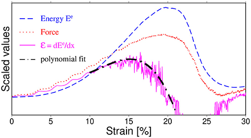
Figure 4. An example of simulated loading curves and the illustration of the procedure of estimation of maxima of F(x) and ${E}$(x) curves by means of a polynomial approximation. The maximum of ${E}$(x) is found by fitting a 3rd order polynomial to an appropriate curve around its noisy maximum. The same procedure was used for getting x_c from F(x).

We have preferred this more complex procedure of estimating the location of the maxima instead of an additional low pass filtering of ${E}$(x) and direct search for it because this way we have avoided an additional phase shift (introduced always by a filtering procedure).

The obtained values of maxima location can, in principle, be used to calculate the δ_x parameter. However, such a direct approach unavoidably leads to loss of estimation precision. Since this parameter is the most important for our analysis, we have thus used yet another, more advanced Bayesian approach [31] capable to explore information about δ_x provided by a given dataset in the optimum way. The details of the method can be found in, for example, Tarantola [31] and Debski [32] and here let us recall only the most important points of the method.

A task of estimating the unknown parameters (here δ_x) from a given data set can be cast into a task of joining of the whole available information about the thought parameters. This information comes from observation (data) theory (relation between thought and measured quantities) and a priori existing estimations. The important fact is that all information contributing to the final estimation is essentially imprecise. Thus, first of all any data are subjected to uncertainties due to the limited accuracy of any measurement/simulation. Theoretical uncertainties arise from possibly approximate relations between thought parameters and those which have been measured or simulated. Finally, the existing (if at all) a priori information is often quite vague.

From the mathematical point of view, the idea of joining information is formulated using the Bayesian interpretation of probability [33]. It takes the form of constructing the so-called a posteriori probability distribution, which in the most often met situations reads [31, 32]

$\begin{array}{ll}\sigma (m)=f(m)exp\left(-\left|\right|da{t}^{obs}-dat(m)\left|\right|\right),& (25)\end{array}$

where m stands for the thought parameters, dat^obs and dat(m) are observational data and theoretical prediction for a given m, and ||·|| stands for a norm measuring a “distance” between observations and predictions. Finally, the f(m) is a probability distribution describing our a priori knowledge. It can be proved [31] that σ(m) provides the quantitative description of all available information about m.

An application of this approach for estimation of the δ_x parameters takes a few steps. First, we identify m with δ_x: m = δ_x. Next, as “observational” data we chose the function F(x). Finally, we have assumed that around their maxima the F(x) and ${E}(x)$ curves are similar enough so locally one can write

$\begin{array}{ll}F(x)\approx const.{E}(x+\delta x).& (26)\end{array}$

This last assumptions simply tells that the peak of ${E}(x)$, when scaled and shifted by δ_x, should coincide with the peak of F(x). One can try to provide deeper arguments for such assumption, based, for example, on the FBM prediction (see Figure 3), but in our case it basically follows from the observation of an occurrence of such coincidences (see, e.g., the upper left panel in Figure 5).

FIGURE 5

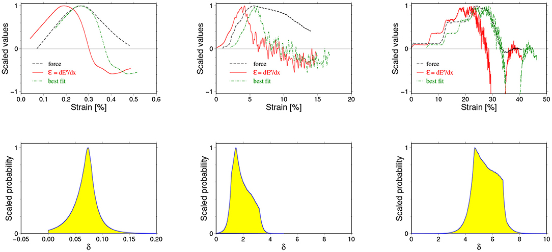
Figure 5. Three examples of an estimation of the delay parameter δ_x using the Bayesian (probabilistic) approach. The curves F(x), ${E}$(x), and ${E}$(x+δ_x) for the optimal δ_x value are shown in the upper row. The lower row shows corresponding a posteriori probability distributions. The shown cases correspond to one of the best (almost noise-free) simulation results (left column) with well matching F and ${E}$ curves, a typical situation (middle column) and a “difficult” case when acoustic waves strongly disturbed the breaking process.

The choice of the norm ||·|| in Equation (25) should reflect the expected observational and theoretical uncertainties [32]. In cases of tasks with “data” represented by continuous functions, the cross-correlation of dat^obs and dat(m) is most often used. However, we have preferred another choice, namely

$\begin{array}{ll}\left|\right|da{t}^{obs}-dat(m)\left|\right|={\displaystyle \sum _i}|F(x_i)-{E}(x_i+\delta x)|,& (27)\end{array}$

where |·| stands for the absolute value and the sum is over all strain values in predefined range. This l₁-based norm is more robust than the classical cross-correlation norm (essentially equivalent to least-squares norm) and easily accommodates even large differences for a finite number of x_i arguments [32]. However, if one or both curves have large gradients within the summation range using such norm can lead to seriously biased a posteriori probability distribution [31]. In consequence, estimated solutions can also be subjected to uncontrolled systematic errors.

While plotting the output results we used the convention according to which a vertical elongation of the sample (strain) was expressed by percentage of an initial sample height, i.e.,

$\begin{array}{ll}x=\frac{l-l_0}{l_0}\times 100\%& (28)\end{array}$

To enable the visualizations all plotted quantities, like elastic energy E^e, its derivative (${E}$), and stretching force F, etc., were separately normalized.

5. Results

The performed simulations have provided numerical evidence that can be used to support or falsify the FBM prediction, thus being a proxy of experimental measurements. Adopting this point of view and by analogy to real experiments, the important question arises about uncertainties inherent to the simulation results. The simulations provide us with macroscopic quantities, like total elastic energy absorbed by the sample and stored in inter-particle bonds, deformation of the sample, number of broken bonds, and total force acting on the upper, moving up plate. They also provide data allowing to construct snapshots of microscopic state of the sample at any time during the simulation. Each of these quantities is subjected to uncertainties coming from different sources. We have identified three of them, namely numerical errors, statistical fluctuations and effects of additional physical processes. Since the last issue is strictly connected with observed breaking mechanisms, we describe uncertainty and breaking mechanism analysis together.

5.1. Uncertainty Analysis

Numerical simulations, depending on the assumed aims, can be viewed either as an extension of theoretical analysis toward situations that cannot be treated analytically due to the complexity of the problem or as an extension of experimental data. This double point of view causes some controversy with respect to how numerical errors should be treated. The first (modeling) approach concentrates only on achieving the highest possible theoretical accuracy as numerical simulations are treated as a direct extension of the underlying theory. The error analysis is in this case straightforward and concentrates on such issues as the accuracy of the approximations to the underlying equations and the stability of the numerical scheme that, by the way, can be quite complex from a technical point of view. On the other hand, if the simulation is to provide observational data, we need a much broader approach to the uncertainty analysis. We have to include not only the issue of numerical uncertainties, but also characteristics of the simulated processes. This essentially complicates matters.

The DEM method, like any other numerical implementations of analytical models, has limitations and introduces unavoidably some approximations resulting in numerical uncertainties. The two most important factors are at present an accuracy of approximations of derivatives in original continuous physical equations and the stability of the time integration [34]. The last issue has generated much attention and has lead to the formulation of various so-called stability conditions (see, for example [9] for an analysis). Their basic meaning is to assure that none of the particles constituting the sample move too far from their current positions in a single time step. If such motion should happen, the interactions with neighborhood particles will lead to extremely large, non-physical forces acting between neighboring particles and as a consequence generate spurious high-frequency oscillations or even blowing up the whole sample. This instability is in fact the main source of numerical noise in DEM simulations and can be controlled (diminished) by choosing appropriately small time steps. However, it is very difficult to completely get rid of this type of noise, especially if the simulations contain large numbers of particles. In such systems, there is always a finite chance that at a given evolution stage, internal forces will exceed the stability limit due to fluctuations and the particles (especially the smallest ones) will locally start high frequency oscillations. However, in many cases such artificial oscillations are quite efficiently dumped by the interactions with surrounding particles during the next couple of time steps. If there remains as stationary noise, the simulation can often be accepted and noise can be removed by standard low pass data filtering. We refer to this particular feature of DEM as soft stability.

The significant feature of the performed simulations is their multi-body character. We model the behavior of a system of a large number of interacting objects. We would then expect the occurrance of statistical fluctuations in the macroscopic variables, such as drag force, elastic energy, etc. From our point of view, such fluctuations can be treated as a noise disturbing the simulation results.

The last identified source of final uncertainties was the fact that the DEM simulations inherently include the geometry of the sample and (implicitly) the finite speed of stress and strain development inside it. In consequence, we have always simulated not only a “pure” breaking process but also additional physical processes, among which generating of acoustic waves and stress diffusions were the most important. Under some favorable conditions, these additional physical processes seriously influenced our simulations and have not allowed to identify the critical value at all. In most cases, however, they only significantly contributed to the final, a posteriori uncertainties.

The described types of simulation uncertainties are presented in Figure 6, where examples of numerical noise, statistical fluctuations and creation of acoustic waves and their influence on observed parameters are shown. In addition, we include in this figure (middle row) the a posteriori distributions for the δ_x parameter estimated for the presented cases and examples of snapshots of the internal state of the samples illustrating mechanisms of generation of a given type of noise. For the purpose of this illustration, we adopted special measures. First of all, we have slightly increased the numerical noise (left column in Figure 6 by enlarging the time step in this case. Moreover, we have started this simulation with abrupt loading which has led to some minor instabilities already at the beginning of simulation. These continued as stationary high frequency noise. On the other hand, to illustrate statistical fluctuation type noise (middle column) we have decreased the evolution time step to diminish the numerical noise and also have gently started loading. In the last cases (right column), no special measures have been applied.

FIGURE 6

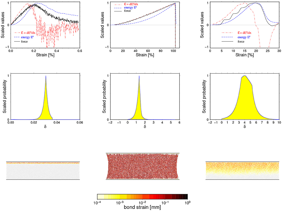
Figure 6. Three types of noise encountered in performed simulations: numerical noise (left column), statistical fluctuations (middle column), and disturbances due to additional physical processes (right column). The F(x), ${E}$(x), and E^e(x) curves are shown in the uppermost row, the corresponding a posteriori probability distributions for δ_x parameter in the middle one, and selected snapshots of samples micro-structures in the lower-most row. The snapshots show the inter-particle bonds strains and use the same color scale. See text for detailed explanations.

A few conclusions can be drawn from Figure 6. First of all, we observe that the numerical noise and statistical fluctuations lead to quite similar effects: a high frequency, low amplitude oscillation visible in the F(x) and ${E}$(x) curves. In practice, these two types of noise are indistinguishable. On the other hand, the existence of acoustic waves leads to a characteristic undulation of the F(x) curve and, in the presented case, has significantly masked the critical value and decreased the accuracy of the estimation of x_c. The conclusion is that a low-pas filtering of the data can efficiently remove numerical and fluctuation noise, but not errors introduced by additional physical processes.

Secondly, the numerical noise can appear at any stage of evolution and can hardly be visible as a disturbance of the microscopic state (provided we are within a soft stability limit). On the other hand, the statistical fluctuations appear only if the sample has accommodated enough elastic energy uniformly distributed over the whole sample making the system reach a quasi-equilibrium state. The existence of acoustic waves is clearly visible in the snapshots as a time propagating disturbance.

The most interesting is, however, a comparison of the a posteriori distribution for δ_x parameters estimated by the Bayesian inversion method (middle row in Figure 6) which brings us information on how to identify how a given type of noise influences the δ_x estimation. In all cases we have observed a unimodal distribution whose shape essentially follows the l₁ norm-based likelihood function we have used. The “width” of this distribution is a measure of the accuracy of δ_x estimation. The smallest uncertainties are (or can be) due to the numerical noise. The statistical fluctuations lead to larger, though still moderate uncertainties. Finally, the largest errors are potentially introduced by the acoustic waves. Although the presented cases are for illustration only and hence arbitrary chosen, they suggest that the most important source of the final uncertainties are acoustic waves, or more generally, additional physical processes accompanying the breaking process in the DEM simulation [30]. In the next section, we discuss, among other issues, the contribution of the different observed breaking mechanisms to the types of noise.

Finally, let us note that the contribution of the numerical noise is not only small if the simulation is properly run, but in principle it can be highly suppressed by reducing the time step used. In practice, the reducing of time steps leads to much longer, often unacceptable computations, so that some level of numerical noise has to be accepted. Although it can easily be removed by low pass filtering, it marks its existence in a posteriori errors. It is not clear how the influence of statistical fluctuations on the final uncertainties can be diminished. A more advanced analysis, taking into account the possibility of resizing the sample, is apparently needed in this case. Finally, the uncertainties due to additional physical processes seems to be irreducible and the only way of avoiding them is a proper selection of the simulation setup.

5.2. Breaking Mechanisms

Within the set of performed simulations we have observed a variety of different breaking mechanisms. Some of them were qualitatively quite similar to the FBM predictions illustrated in Figure 3, and some were apparently quite different. The observed difference in simulated breaking processes were obviously due to different values of the (k_n, b_d) parameters because all others conditions (micro-structure of the sample and loading conditions) were kept the same. It is thus obvious that the richness of breaking modes arises directly from a non-linearity of the breaking of particle-particle bonds controlled by (k_n, b_d). However, we have to point out an important role of microscopic structure of the sample in a fragmentation process. Actually, for a given virtual material defined by (k_n, b_d) an actually breaking process is determined by a micro-structure of the sample—a particle distribution in the sample. It determines which bonds break first, in which direction a fracture tip progress, etc. In our case the particles are distributed randomly and the sample is heterogeneous at the particles level. It introduces some randomness to our simulations. In principle, it is the same for all performed simulations because we have always used the same sample. However, in reality it is not exactly a case because the micro-structure of the sample is continuously changing from the time the first particle-particle bond breaks. The complex, non-linear feedback between a pair of (k_n, b_d) parameters and the internal micro-structure during the breaking process causes that at the breaking stage we are efficiently dealing with slightly different samples for different (k_n, b_d) parameters.

For the purpose of our analysis we divide the observed breaking mechanisms qualitatively in the following into four categories, shortly describing their main features.

The first class of observed breaking mechanisms, referred to as ductile-like, is characterized by a very wide maximum of elastic energy around the failure point x_c. An example of variation of the force, elastic energy and its derivative with the sample deformation is shown in Figure 7. This figure also provides a histogram illustrating the change of the rate of bond breaking during the simulation. Three snapshots of the sample's internal state illustrating this breaking mechanism ares shown in Figure 8.

FIGURE 7

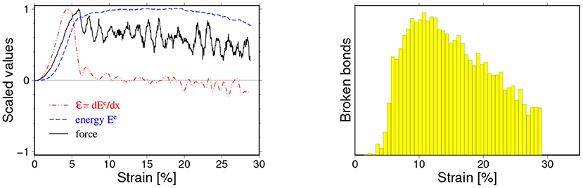
Figure 7. An example of the ductile-like breaking mechanism. (Left) Force (F)—thick black curve, Elastic energy (E^e)—thin blue solid curve and the energy absorption rate (${E}$)—dashed red curve as functions of strain x. (Right) number of broken bonds in a fixed strain interval against x. A relatively fast increase of elastic energy at an initial phase is followed by a long-lasting stage of slowly changing elastic energy (left). At this stage, a slow destruction of the sample is observed (right) and the loading force needed to keep stretching speed constant exhibits significant fluctuations. The particle-particle interaction parameters for this case read: k_n = 10⁷ N/mm, b_d = 0.01 mm.

FIGURE 8

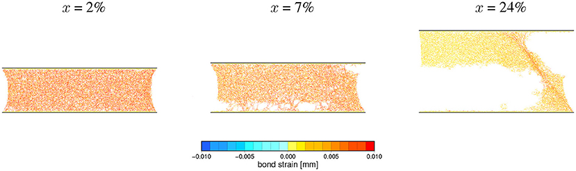
Figure 8. Snapshots of the microscopic state of a sample undergoing a ductile-like breaking process at strains (x = 2, 7, 24%) indicated above the panels. Short colored segments represent inter-particle bonds existing at a given loading stage and their extension with respect to initial values are mapped by colors. The corresponding loading curves are shown in Figure 7.

For this type of simulated breaking process, we observe a fast initial absorption of external work and nucleation of fracturing followed by a very slow destruction of the sample. During this continuous damage stage, the force needed for keeping the constant stretching speed exhibit significant fluctuations with many local maxima. The breaking process was apparently much more complex than predicted by FBM (Figure 3). For this type of breaking mechanisms, it was impossible to identify the critical strain x_c at which samples reached the unstable phase. For this reason we have not considered such cases in analysis that follows. It is interesting, however, that even in this case the energy absorption rate curve demonstrated a well-defined maximum, which appeared prior to any loading force maximum as visible in Figure 7—following in a sense the FBM predictions.

The second class of observed fracture process consists of brittle-like processes during which collapse of the sample occurred very quickly after the beginning of loading without a visible “necking” of the sample. They always have a form of tearing out a few uppermost (or lower-most) layers from the remaining body of the sample in a cleavage-like process. Figure 9 shows a post-failure state of the sample broken this way and Figure 9 the corresponding loading curves and broken bonds. Apparently, such a breaking scenario is most similar to the one modeled by the FBM (Figure 3). An additional advantage of this breaking mechanism is that a relatively high accuracy of the δ_x estimation may be achieved due to neither statistical fluctuations nor acoustic waves have adequate room for development. However, such cases require a very gentle beginning of loading to avoid numerical instabilities.

FIGURE 9

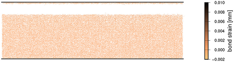
Figure 9. Snapshots of a microscopic state of a sample undergoing a pure brittle cleavage-like breaking process. Short colored segments represent the inter-particle bonds existing at a given loading stage and their extension with respect to the initial values are mapped by colors. The corresponding loading curves are shown in Figure 10.

FIGURE 10

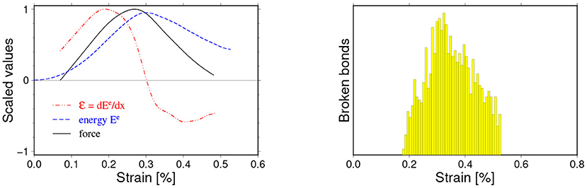
Figure 10. An example of loading curves for the pure brittle cleavage-like breaking mechanisms (see Figure 7 for the description). In this case, the fracture occurs at very small deformations and is very well-localized around the critical strain x_c. The particle-particle interaction parameters for this case read: k_n = 10 N/mm, b_d = 0.1 mm.

The collapse of the sample occurred at very small strains and happened very quickly as a result of the bonds were breaking only in a narrow strain range around a well-pronounced critical value x_c. The energy absorption rate curve ${E}$(x) has its maximum ahead of the critical strain x_c. We have observed mechanisms of this type only for the smallest values of critical bonds strains b_d < 0.1mm regardless of the considered values of k_n.

In many simulations we have observed a breaking mechanism referred to as hyper-elastic. In a way similar to the brittle cases, the damaged energy is released in a small well-localized region around x_c. What distinguishes this scenario from the brittle scenario is a long initial stage of building-up the internal elastic energy of the sample and as a consequence a significant necking of the sample prior to breaking, typical for real ductile materials. Figure 11 shows loading curves for such cases, and a sequence of snapshots characteristic for this type of breaking process is shown in Figure 12.

FIGURE 11

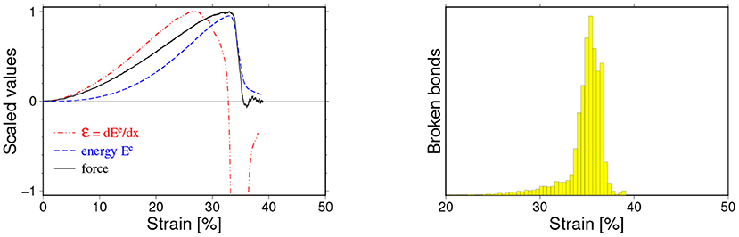
Figure 11. Loading curves for the hyper-elastic breaking mechanisms (see Figure 7 for the description). In this case the fracture has occurred at relatively large deformations but, like in the brittle cases, has been very well-localized around the critical strain x_c, and the accumulated elastic energy is almost entirely and quickly released. The particle-particle interaction parameters for this case read: k_n = 10⁵ N/mm, b_d = 0.4 mm.

FIGURE 12

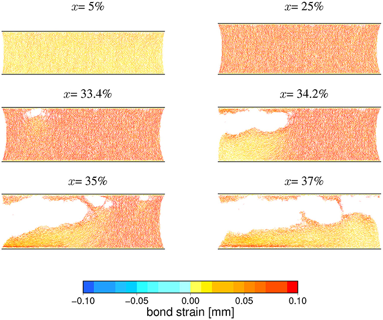
Figure 12. Snapshots of the microscopic state of a sample undergoing a hyper-elastic breaking process at selected (indicated above panels) strains. Short colored segments represent inter-particles bonds existing at given loading stage and their extension with respect to initial values are mapped by colors. The corresponding loading curves are shown in Figure 9. A release of an internal elastic stress by developing fracture system is clearly visible. The particle-particle interaction parameters for this case read: k_n = 10⁵ N/mm, b_d = 0.4 mm.

Apparently as Figure 12 demonstrates, in such cases we are encountering a more complex breaking process than what is described in the FBM. However, in spite of this, the basic features of the failure process seen in the FBM are still preserved. For this type of fracturing we observe a well-pronounced peaks of F(x), ${E}$(x), and usually a delayed but also well visible wider peak of E^e(x). Only in such cases a favorable conditions for developing statistical fluctuations occurred, because the sample (depending on values of microscopic parameters k_n, b_d) could absorb and store a large amount of internal energy. Simulations leading to this type of breaking process were quite susceptible to generating numerical noise which usually appeared around the critical value because at this stage the internal forces approaches their maximum values and numerical instabilities could easily develop. If such a noise was stationary or was diminishing, the simulation was accepted. Otherwise, the simulation was repeated with a smaller time step. In some cases, especially for cases with shorter initial stable phase we observed the development of acoustic waves propagating through the sample. However, the energy they were carrying was much smaller than the accumulated elastic energy, so their existence practically lead to some increase of final uncertainty only.

The final class of the observed mechanisms can be referred to as semi-ductile. One of the distinct features of events of this class is the presence of clearly visible acoustic waves in the stable loading phase. In some cases they lead to a small undulation of F(x), E^e(x) or its derivative. However, in some cases they can completely dominate the loading phase of the evolution. In such extreme cases they can even prohibit a precise identification of the critical stretch. The loading curves for such an extreme case when strong acoustic waves have been generated from the beginning of the process is shown in Figure 13.

FIGURE 13

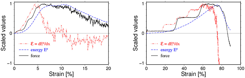
Figure 13. Two examples of loading curves for semi-ductile breaking mechanisms with moderate (left) and strong amplitude acoustic waves generated and developing from the beginning of loading (see Figure 7 for the description). The wavelength of the acoustic waves for the case shown in the left panel is about 1/3 of critical strain and their presence manifest themselves in irregular increase of the loading force in the initial loading stage strain. In the case shown in the right panel neither the critical stress x_c nor the maximum of energy absorption rate can be found with acceptable accuracy due to the strong acoustic waves. The particle-particle interaction parameters for the case shawn on left read: k_n = 10⁵ N/mm, b_d = 0.05 mm and for the case shown on right k_n = 10² N/mm, b_d = 0.6 mm.

For events of this class we still can identify the critical value, and the maximum of the energy absorption rate but often with much lower accuracy. The E^e(x) curves are quite wide and their maxima are often noticeably shifted toward larger x with respect to x_c similar to ductile cases. However, unlike the ductile cases, F(x) is relatively smoothly decaying with increasing x. The slowly decreasing of the elastic energy after reaching the critical value indicates a complex breaking mechanism. Indeed, we observe for such cases, the failure goes through the development of a multi-crack-systems. The micro-crack interact with each other and coalesce, which finally leads to a failure of the sample. This breaking mechanism is much slower than the fracturing process typical for hyper-elastic cases (fast horizontal fracture) or brittle one (cleavage process). The series of snapshots shown in Figure 14 illustrates both above mentioned features.

FIGURE 14

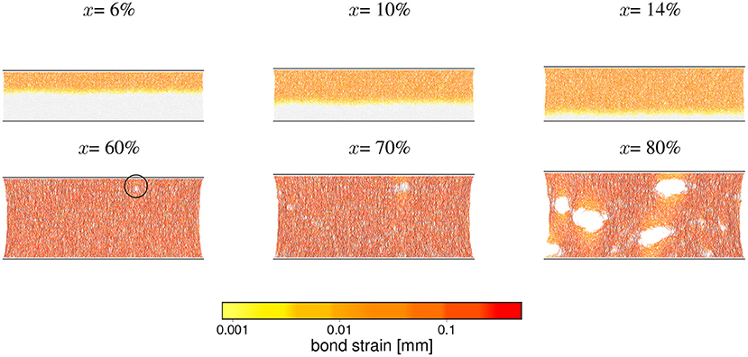
Figure 14. Snapshots (at indicated deformations x) of the microscopic state of a sample undergoing a semi-ductile breaking process. The corresponding loading curves are shown in right panel in Figure 13. The most essential features for this class of processes are: (a) the development and propagation of acoustic waves (upper row) and (b) multi-crack fracturing pattern (lower row). The first visible signature of development of the fracture system, appearing at about 60% strain is marked by a circle in the lower left panel and at 80% strain the sample is still far away from breaking apart. Such a slow failure process is typical for this class of processes and differentiates it from hyper-elastic ones (see Figure 12). The particle-particle interaction parameters for this case read: k_n = 10² N/mm, b_d = 0.6 mm.

All analyzed DEM simulations are finally shown on the scatter plot in Figure 15. The four categories of breaking mechanisms are represented at this figure by different colors. In spite of the fact that the proposed categorization is merely qualitative conclusions are quite obvious. The brittle-like processes are observed only for weak (small k_n) and rigid (small b_d) virtual materials. On the other hand the hyper-elastic cases were observed for stronger (large k_n) but flexible (large b_d) materials. The semi-ductile cases were observed for intermediate values of the (k_n, b_d) parameters with a probably (insufficient space sampling) smooth transition toward the ductile type in a region of small b_d and large k_nparameters. Star symbols are used to distinguished at Figure 15 cases for which the maximum of elastic energy is a significantly delayed (Γ > 5) with respect to the critical strain. Surprisingly, within the given set of simulated cases such events are mostly located along the brittle—semi-ductile boundary. This issue will be analyzed elsewhere.

FIGURE 15

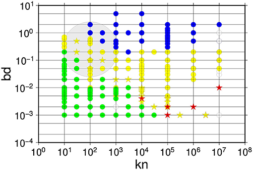
Figure 15. The scatter plot of all analyzed events on the k_n-b_d plane. Different colors represent different categories of observed breaking mechanism: green—brittle, blue—hyper-elastic, yellow—semi-ductile, red—ductile, respectively. The star symbols depict cases for which the maximum of elastic energy is significantly delayed (Γ > 5) with respect to the critical strain. For few cases we could not determine (for technical reasons) the delay parameter Γ and such cases are left as open (white) circles. The region of (k_n, b_d) parameters for which strong acoustic waves were observed is shaded in gray.

5.3. Signature of Imminent Failure

Answering the main question posed at the beginning of this paper, let us begin the discussion of results by gathering the information on the δ_x parameter from all analyzed numerical simulations. The result is shown in Figure 16.

FIGURE 16

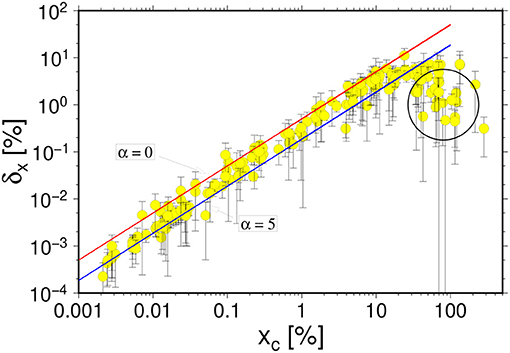
Figure 16. The delay δ_x = x_c − x_p between the critical stress x_c and the strain at which the elastic energy absorption rate reaches maximum for all but ductile-like simulation results. The dashed curves show the FBM predictions for power law distributions with α = 0 and 5. The circled events show systematically underestimated δ_x values due to used procedure of δ_x calculation (see text for details).

The most obvious conclusion from this figure is that within the class of analyzed events we have always observed a positive value of δ_x. Estimated uncertainties indicate the significance of this result. It holds for all observed critical strains x_c. We observe the monotonic, almost linear increase of δ_x with x_c over the range 0.01 < x_c < 10. Distortions observed at the smallest x_c are most probably due to the resolution limit imposed by a necessity of using a low pass filter to remove noise. Much more interesting is a saturation of δ_x(x_c) at large x_c. Actually, two effects are visible for the largest x_c values. The first one is the existence of a group of events for which δ_x values are significantly smaller than the remaining ones. This group is circled in Figure 16. A closer inspection of breaking mechanisms for this group of events reveales that all have the same breaking pattern shown at the uppermost, middle panel in Figure 6. For such curves with large gradients the used method of constructing the likelihood function often fails [31] and leads to serious under-, or overestimation of the parameters. This is exactly the case for this group of events.

It could have been corrected, however we have not done it since it would go beyond the main goal of the paper and was of relatively low importance for the group of events we analyzed. Besides this technical issue, we observe an apparent saturation of the δ_x(x_c) curve. This effect may have different origins. One of them can be a finite size of the used sample. We are also recall a limitation of the DEM method in connection with a proper description of materials with large Poisson ratios [35]. However, it can also be a signature of approaching the limits of applicability of the FBM model. This issue requires further investigations.

The visible deviations at extremely small and large x_c do not, however, change the main conclusions, that for over three orders of magnitude of x_c the numerical DEM results are in a very good agreement with the FBM predictions concerning the positivity of δ_x and its dependence on x_c. The obtained results fits perfectly with the FBM predictions for power law fiber strength distributions with exponents in the range 0 < α <5.

We provide complementary information and independent support for the FBM predictions in the plot of the A^r coefficient against x_c, as shown in Figure 17. We have here plotted it dividing all events into three categories with respect to the Γ parameter. Let us recall here that according to Equation (17) this dimensionless parameter measures the retardation of the point when internal elastic energy reaches a maximum value with respect to the critical value x_c. The larger the parameter Γ, the latter the elastic energy maximum, and the wider a peak of the elastic energy. Two curves corresponding to the FBM predictions for the power law distributions with exponents α = 0, and5 are also shown.

FIGURE 17

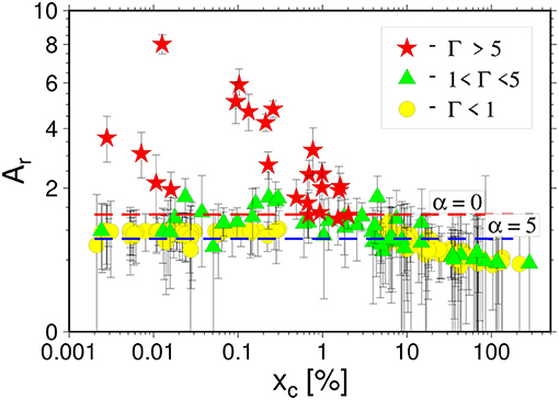
Figure 17. The ratio A^r of the maximum of elastic energy released during the final failure to the product of maximum of elastic energy increase rate and x_p against x. Horizontal lines shows the prediction of the FBM model for power distribution with α = 0—red line and α = 5—blue line. Errors are mainly due to imprecise estimation of x_p and ${{E}}_{max}$. The plotted values have been divided into three groups depending on the value of Γ expressing the retardation of the energy maximum x_m with respect to x_c (see Equation 17): the maximum of energy just follows the x_c point (Γ < 1), intermediate case (1 < Γ < 5) and the case when the energy maximum occurs far away from x_c.

For the majority of events characterized by the critical strain x_c lower than about 10% we have obtained an almost constant value of A^r in full compliance with the FBM predictions (see Equation 23). The agreement for the power law distribution with exponents in the range 0 < α < 5 is remarkably good, and the range of α for which it holds agrees with the analysis for δ_x. In the case of A^r we also observe a systematic deviations from the FBM model for the largest x_c. The reasons for this deviation are most probably the same as in the case of δ_x parameters and will be discussed elsewhere.

The most intriguing result shown in Figure 17 is, however, the existence of a group of events for which values of A^r are much larger than 4/3, i.e., the value predicted by FBM as the superior limit. For these few exceptional events we have observed A^r ~ 3 and Γ over 5, (the FBM prediction is Γ < 1), thus much beyond the FBM limits. It has to be noticed that these exceptional events appear at critical strains for which other, compliant with FBM solutions exist and they are not influenced by the data processing methods, which was the case for the δ_x parameter for the largest x_c. Detailed examination of the loading curves and the snapshots of the breaking process have indicated that all these events exhibit semi-ductile, complex breaking mechanism, and that is why their common feature are large values of Γ. It is thus not astonishing that they do not fit the FBM predictions for which the breaking mechanism is a simple “one-step” process. When the critical value is reached the loading process switches from the stable to the unstable phase leading to an immediate breaking of the sample and hence release of the whole reservoir of energy. It is astonishing that for this group of events, the deviation from the FBM prediction for A^r we observe simultaneously no departures from the FBM results concerning the positivity of x_c. Actually, observation of the existence of such events is one of the two most important results of our analysis.

6. Discussion and Conclusions

Considering the posed question whether the signature of imminent failure predicted by the FBM method is also visible in the DEM simulations, we can positively answer yes. In all analyzed simulations we observe the existence of a precursory maximum of an elastic energy absorption rate prior to the critical strain at which the loading force reaches the maximum. We have also observed a very good agreement of the DEM simulation results with the FBM predictions for the variation of the δ_x–a difference between the critical strain and the strain at which precursor maximum occurs, and the A^r–the scaled ratio of total absorbed energy and maximum of the absorption rate parameters. The advanced error analysis allows us to recognize and qualitatively take into account the sources of major errors providing solid evidence for the above conclusions. All these arguments provide a strong support for the Fiber Bundle Model. However, a few observed facts forces us to pose some important physical questions and prevent us from drawing too optimistic but possibly too naive conclusions.

The first issue is a possible bias/limitation introduced by the selection procedure we have applied to the DEM simulations. We have considered only cases with a well-pronounced peak in the force and the energy absorption rate curves. The motivation of such selection is purely technical—we wished to assure a satisfactory accuracy of identifying of the critical value and the point at which the energy absorption rate reaches maximum. Among almost 200 performed simulations, only eight have been rejected due to failing this condition, which suggests it to be quite reasonable. However, consequences of such a procedure, even if it looks reasonable, go much beyond the technical issue itself. Actually, the applied criterion resulted in restriction of our analysis to processes in which force, energy absorption rate, and also elastic energy (although it was not required) were single-modal. By this we understand that the corresponding loading curves were quite compactly localized around the critical strain and do not exhibit a presence of significant secondary local maxima. What is the physical meaning of this fact?

The well-pronounced single, peaks in force, elastic energy, and energy absorption rate function mean that the breaking is essentially a “one-step” process. When initiate at the critical strain it unavoidably leads to a breaking of an object apart and release of the whole absorbed and stored internal energy. For such cases, the DEM simulations indeed confirm the existence of a precursory phenomena preceding the imminent failure, as predicted by FBM [5]. The DEM simulations have shown that this phenomenon also holds if more complex, but still essentially “one-step” processes are considered. The situation changes essentially if more complex breaking processes are considered. The existence of such processes has recently been reported [30] and in a restricted form of semi-ductile cases also appeared in our simulations. For such processes we found a “soft” breaking the FBM predictions: the A^r, and Γ parameters significantly differs from the FBM predictions but the δ_x parameter follows closely the FBM solution. An open question thus arises if the existence of the precursor phenomenon predicted by FBM can still be observed in case of more complex processes or not. For example, one can imagine the breaking process consisting of a series of smaller sub-failures. Will the system inform us about an approaching final failure in such a case? The answer is open.

Another, more elementary issue is related to how the external work done by the loading forces is absorbed and stored in the sample. In the fiber bundle model, the whole work is absorbed as elastic energy of the stretched fibers. Upon breaking a fiber, the elastic energy it has stored is released as the damage energy [5] and, what is important, it decouples from the model. By this we mean that the released energy does not influence the state of remaining fibers. In the DEM method, the situation is more complex. The energy released by a bond breaking is, in the first step, converted directly to the kinetic energy of particles originally joined by the bond. In the next steps, this “damage” energy either transforms (most of it) into elastic energy of remaining bonds attached to particles or remains to be a kinetic energy of vibrating particles. The first situation occurs if particles can hardly move or if they can carry a minimum kinetic energy due to their small masses. If this situation occurs, DEM directly mimics the FBM approach. However, DEM can also simulate an opposite situation, when the released energy can (to some extent) remain as kinetic energy of the originally bonded particles [30] and so does not decouple from the system. The obvious questions to be answered in the future are how such elastic-kinetic energy conversion mechanism modifies the FBM predictions, is this process responsible for the complexity of ductile-like breaking process, and so forth.

In the light of the above comments, the results of our analysis can be summarized in a general way as follows: When the external force is stretching a body, part of its work (all in an ideal case) converts into the internal energy of the body. If this energy transfer is dominated by building up an elastic energy and the final breaking of the body is a single-step process, then we observe a robust signal-precursor of the upcoming failure. The reaching of the maximum by the elastic energy absorption rate is just a signature that a catastrophic failure is approaching. The obtained results immediately poses further important questions. The first, and the most important one is, what are the limits of applicability of the FBM method when applied to description of breaking solid materials. Another one is whether the inclusion of mechanisms of conversion of the external work into kinetic energy (heat) of particles/fibers change the conclusion about relation between the maximum energy absorption rate and the critical value or not.

Data Availability Statement

The raw data supporting the conclusions of this article will be made available by the authors, without undue reservation.

Author Contributions

WD performed the DEM simulattions. SP and AH performed the FBM analysis. All authors equally contributed to data analysis and interpretations as well as preparing the manuscript.

Funding

This work was partially supported by the Research Council of Norway through its Centers of Excellence funding scheme, project number 262644. This research was supported in part by a subsidy from the Polish Ministry of Education and Science for the Institute of Geophysics, Polish Academy of Sciences.

Conflict of Interest

The authors declare that the research was conducted in the absence of any commercial or financial relationships that could be construed as a potential conflict of interest.

References

1. Reiweger I, Dual JSJ, Herrmann HJ. Modelling snow failure with a fibre bundle model. J Glaciol. (2009) 55:997. doi: 10.3189/002214309790794869

CrossRef Full Text | Google Scholar

2. Cohen D, Lehmann P Or D. Numerical modelling of riverbed grain size stratigraphic evolution. Water Resour Res. (2009) 45:W10436. doi: 10.1029/2009WR007889

CrossRef Full Text

3. Pollen N, Simon A. Estimating the mechanical effects of riparian vegetation on stream bank stability using a fiber bundle model. Water Resour Res. (2005) 41:W07025. doi: 10.1029/2004WR003801

CrossRef Full Text | Google Scholar

4. Pugno NM, Bosia F, Abdalrahman T. Hierarchical fiber bundle model to investigate the complex architectures of biological materials. Phys Rev E. (2012) 85:011903. doi: 10.1103/PhysRevE.85.011903

PubMed Abstract | CrossRef Full Text | Google Scholar

5. Pradhan S, Kjellstadli JT, Hansen A. Variation of elastic energy shows reliable signal of upcoming catastrophic failure. Front Phys. (2019) 7:106. doi: 10.3389/fphy.2019.00106

CrossRef Full Text | Google Scholar

6. Hansen A, Hemmer PC, Pradhan S. The Fiber Bundle Model. Veinheim: Wiley-VCH (2015). doi: 10.1002/9783527671960

CrossRef Full Text | Google Scholar

7. Cundall PA. A computer model for simulating progressive, large-scale movement in blocky rock systems. Proc Symp Int Soc Rock Mech. (1971) 2:2–8.

Google Scholar

8. Peirce FT. Tensile tests for cottom yarns. “The weakest link” theorems on the strength of long and composite specimens. J Text Ind. (1926) 17:355. doi: 10.1080/19447027.1926.10599953

CrossRef Full Text

9. O'Sullivan C. Particulate Discrete Element Modelling, a Geomechanics Perspective. New York, NY: Routledge; Taylor and Francis Group (2011).

Google Scholar

10. Chakrabarti BK, Benguigui LG. Statistical Physics of Fracture and Breakdown in Disordered Systems. Oxford: Oxford University Press (1997).

Google Scholar

11. Herrmann HJ, Roux S. Statistical Models for the Fracture of Disordered Media. Amsterdam: Elsevier (1990).

Google Scholar

12. Biswas S, Ray P, Chakrabarti BK. Statistical Physics of Fracture, Breakdown, and Earthquake. Berlin: Wiley-VCH (2015). doi: 10.1002/9783527672646

CrossRef Full Text | Google Scholar

13. Daniels HA. The statistical theory of the strength of bundles of threads. Proc Roy Soc A. (1945) 183:243. doi: 10.1098/rspa.1945.0011

CrossRef Full Text | Google Scholar

14. Pradhan S, Hansen A, Chakrabarti BK. Failure processes in elastic fiber bundles. Rev Mod Phys. (2010) 82:499. doi: 10.1103/RevModPhys.82.499

CrossRef Full Text | Google Scholar

15. Sornette D. Elasticity and failure of a set of elements loaded in parallel. J Phys A. (1989) 22:L243. doi: 10.1088/0305-4470/22/6/010

CrossRef Full Text | Google Scholar

16. Hemmer PC, Hansen A. The distribution of simultaneous fiber failures in fiber bundles. ASME J Appl Mech. (1992) 59:909. doi: 10.1115/1.2894060

CrossRef Full Text | Google Scholar

17. Pradhan S, Hansen A, Hemmer PC. Crossover behavior in burst avalanches: signature of imminent failure. Phys Rev Lett. (2005) 95:125501. doi: 10.1103/PhysRevLett.95.125501

PubMed Abstract | CrossRef Full Text | Google Scholar

18. Pradhan S, Hemmer PC. Relaxation dynamics in strained fiber bundlesi. Phys Rev E. (2007) 75:056112. doi: 10.1103/PhysRevE.75.056112

PubMed Abstract | CrossRef Full Text | Google Scholar

19. Pradhan S, Chakrabarti BK. Precursors of catastrophe in the Bak-Tang-Wiesenfeld, Manna, and random-fiber-bundle models of failure. Phys Rev E. (2002) 65:016113. doi: 10.1103/PhysRevE.65.016113

PubMed Abstract | CrossRef Full Text | Google Scholar

20. Batrouni GG, Hansen A, Schmittbuhl J. Heterogeneous interfacial failure between two elastic blocks. Phys Rev E. (2002) 65:036126. doi: 10.1103/PhysRevE.65.036126

PubMed Abstract | CrossRef Full Text | Google Scholar

21. Hidalgo RC, Kun F, Herrmann HJ. Fracture model with variable range of interaction. Phys Rev E. (2002) 65:046148. doi: 10.1103/PhysRevE.65.046148

PubMed Abstract | CrossRef Full Text | Google Scholar

22. Harlow DG, Phoenix SL. Approximations for the strength distribution and size effect in an idealized lattice model of material breakdown. J Mech Phys Solids. (1991) 39:173. doi: 10.1016/0022-5096(91)90002-6

CrossRef Full Text | Google Scholar

23. Potyondy D, Cundall P. A bonded-particle model for rock. Int J Rock Mech and Min Sci. (2004) 41:1329–64. doi: 10.1016/j.ijrmms.2004.09.011

CrossRef Full Text | Google Scholar

24. Zhao Z. Application of discrete element approach in fractured rock masses. In: Shojaei A, Shao J, editors. Porous Rock Fracture Mechanics. Woodhead Publishing (2017). p. 145–76. doi: 10.1016/B978-0-08-100781-5.00007-5

CrossRef Full Text | Google Scholar

25. Egholm DL. A new strategy for discrete element numerical models: 1. Theory. J Geophys Res. (2007) B5:B05203. doi: 10.1029/2006JB004557

CrossRef Full Text | Google Scholar

26. Ergenzinger C, Seifried R, Eberhard P. A discrete element model to describe failure of strong rock in uniaxial compression. Granular Matter. (2011) 13:341–64. doi: 10.1007/s10035-010-0230-7

CrossRef Full Text | Google Scholar

27. Kun F, Varga I, Lennartz-Sassinek S, Main IG. Approach to failure in porous granular materials under compression. Phys Rev E. (2013) 88:062207. doi: 10.1103/PhysRevE.88.062207

PubMed Abstract | CrossRef Full Text | Google Scholar

28. Abe S, Boros V, Hancock W, Weatherley D. ESyS-Particle Tutorial and User's Guide. Version 2.3.1. (2014). Available online at: https://launchpadnet/esys-particle

29. Weatherley D, Boros V, Hancock WR, Abe S. Scaling benchmark of EsyS-Particle for elastic wave propagation simulations. In: 2010 IEEE Sixth International Conference on e-Science, Brisbane (2010). p. 277–83. doi: 10.1109/eScience.2010.40

CrossRef Full Text | Google Scholar

30. Debski W, Klejment P. Earthquake physics beyond the linear fracture mechanics: a discrete approach. Phil Trans R Soc A. (2021) 379:20200132. doi: 10.1098/rsta.2020.0132

CrossRef Full Text | Google Scholar

31. Tarantola A. Inverse Problem Theory and Methods for Model Parameter Estimation. Philadelphia, PA: SIAM (2005). doi: 10.1137/1.9780898717921

CrossRef Full Text | Google Scholar

32. Debski W. Probabilistic inverse theory. Adv Geophys. (2010) 52:1–102. doi: 10.1016/S0065-2687(10)52001-6

CrossRef Full Text | Google Scholar

33. Jeffreys H. Theory of Probability. Oxford: Clarendon Press (1983).

Google Scholar

34. Gottlieb D, Lustman L, Tadmor E. Stability analysis of spectral methods for hyperbolic initial-boundary value problems. J Numer Anal. (1987) 24:241–58. doi: 10.1137/0724020

CrossRef Full Text | Google Scholar

35. Rojek J, Zubelewicz A, Madan N, Nosewicz S. The discrete element method with deformable particles. Int J Numer Methods Eng. (2018) 114:828–60. doi: 10.1002/nme.5767

CrossRef Full Text | Google Scholar