Factors Affecting the Spatial Resolution in 2D Grating–Based X-Ray Phase Contrast Imaging

X-ray phase contrast imaging is a promising technique in X-ray biological microscopy, as it improves the contrast of images for materials with low electron density compared to traditional X-ray imaging. The spatial resolution is an important parameter to evaluate the image quality. In this paper, simulation of factors which may affect the spatial resolution in a typical 2D grating–based phase contrast imaging system is conducted. This simulation is based on scalar diffraction theory and the operator theory of imaging. Absorption, differential phase contrast, and dark-field images are retrieved via the Fourier transform method. Furthermore, the limitation of the grating-to-detector distance in the spatial harmonic method is discussed in detail.

Introduction

In 1895, the X-ray was discovered when Roentgen was engaged in the experiment of cathode rays. Since then, many physicists have been actively studying and exploring the X-ray. The discovery of X-rays has provided an effective means of research in many fields of science. X-ray imaging plays an important role in medical and materials sciences and all other fields that need non-destructive and non-contact detection. The penetration of X-rays makes X-ray imaging a research hotspot. In traditional X-ray imaging, only an absorption image was used. However, as for materials with low electron density, such as soft biological tissues, the contrast remains poor in the absorption image. To solve this problem, X-ray phase contrast imaging was proposed [1]. At the same time, three kinds of images (absorption, differential phase contrast, and dark-field) can be retrieved simultaneously [2]. And the contrast of weak-absorbing materials in the differential phase contrast image is better than that in the absorption image [3]. Among all X-ray phase imaging, the grating-based method is one of the promising solutions to build an imaging system at low cost as it does not need a synchrotron radiation source [4–6]. The microfocal X-ray source [7] or even a traditional X-ray tube can be used as the source [8, 9]. This extends the application of X-ray phase contrast imaging technology [10–13]. In this technique, the spatial harmonic method is a variant grating–based method where absorption, differential phase contrast, and dark-field can be obtained from a single raw image [14–16]. This method could accelerate the imaging speed due to one exposure compared to multiple exposures of the phase-stepping method [15]. And 2D grating is preferred as it could increase the robustness and accuracy of phase retrieval compared with 1D grating [17].

In the X-ray phase contrast imaging system, resolution, sensitivity, and signal-to-noise ratio (SNR) are three important factors related to the image quality. Up to now, many research studies have been conducted toward improving the sensitivity [18]. Birnbacher et al. developed a laboratory X-ray grating-based phase contrast imaging system with 5 nrad sensitivity [19]. Xu et al. discovered that high sensitivity is not always related to high image quality, while the best image quality is achieved at proper sensitivity [20]. As for the signal-to-noise ratio, Fraiz et al. compared SNRs of the retrieved images between two information retrieval methods and found that the angular signal radiography method had a better SNR in refraction and scattering images than the phase-stepping method [21]. Due to the diffraction limit formula, the diffraction limit of X-rays can reach few nanometers. Takano et al. developed a Talbot-Lau interferometer with a Fresnel zone plate (FZP) and built an imaging system which can resolve 50 nm structures in 2017 [22]. Therefore, X-ray phase contrast imaging has much potential in microscopy. According to our investigation, only few research studies were carried out on factors which may influence the spatial resolution of X-ray images.

In this work, we demonstrate a simulation of a 2D grating–based phase contrast imaging system. The simulation is based on scalar diffraction theory and the operator theory of imaging. The factors which may relate to the spatial resolution of three kinds of X-ray images are studied. The spatial resolution in this simulation is evaluated without dose limit in order to ignore the influence brought by the SNR of the system. We also find that when the grating-to-detector distance is chosen with certain values, differential phase contrast could not be retrieved via the spatial harmonic method. The mechanism of this phenomenon is the Talbot effect. The simulation work could be beneficial for setting up an X-ray phase contrast imaging system in demand of high spatial resolution.

Imaging Principle

A typical 2D grating–based phase contrast imaging system is shown in Figure 1A. It consists of an X-ray source, an amplitude 2D grating, and an X-ray detector. Two standard types of 2D grating could be chosen: the checkerboard type, usually with its area duty cycle of 0.5 as shown in Figure 1B, and the mesh type, usually with an area duty cycle of 0.25 as shown in Figure 1C [23].

FIGURE 1

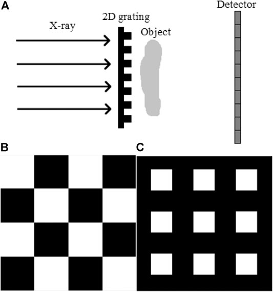
FIGURE 1. A typical 2D grating–based phase contrast imaging system and two types of 2D grating. (A) A typical sketch map of the 2D grating–based phase contrast imaging system. (B) Checkerboard-type 2D grating with the area duty cycle of 0.5. (C) Mesh-type 2D grating with the area duty cycle of 0.25.

In order to elucidate the physical mechanism in X-ray phase contrast imaging, it is assumed that the sample in this system is isotropic. The complex refractive index of the sample could be given as follows:

$n\left(\lambda \right)=1-\delta \left(\lambda \right)+i\beta \left(\lambda \right).(1)$

Here, $\lambda$ is the wavelength of the illuminating X-ray. $\delta$ and $\beta$ are the phase and absorption factor of the sample, respectively, and both vary at different wavelengths. In the imaging system, the distance between the X-ray source and the detector is finite. Therefore, the diffraction occurring in the system can be regarded as near-field diffraction. And the Fresnel diffraction integral under paraxial approximation can be expressed as follows [24]:

${\psi }_{out}\left(\overrightarrow{u_{out}}\right)=\frac{\exp \left(ikz\right)}{i\lambda z}{\displaystyle \iint {\psi }_{in}\left(\overrightarrow{u_{in}}\right)}\exp \left\{\frac{ik}{2z}\left[{\left(x_{out}-x_{in}\right)}^2+{\left(y_{out}-y_{in}\right)}^2\right]\right\}d{x}_{in}d{y}_{in}.(2)$

Here, ${\psi }_{in}\left(\overrightarrow{u}\right)$ represents the electromagnetic wave fields entering the free space. ${\psi }_{out}\left(\overrightarrow{u}\right)$ represents the electromagnetic wave fields exiting the free space. The vector $\overrightarrow{u_{in}}=\left(x_{in},y_{in}\right)$ is the Euclidean coordinates of the point in the input plane. The vector $\overrightarrow{u_{out}}=\left(x_{out},y_{out}\right)$ is the Euclidean coordinates of the point in the output plane.

According to the formula of Fourier transform, Eq. 2 could be expressed as follows [24]:

${\psi }_{out}\left(\overrightarrow{u_{out}}\right)={\psi }_{in}\left(\overrightarrow{u_{in}}\right)\otimes h_{space}\left(\overrightarrow{u_{out}}\right),(3)$

$h_{space}\left(\overrightarrow{u_{out}}\right)=\frac{\exp \left(ikz\right)}{i\lambda z}\exp \frac{ik}{2z}\left(x_{out}^2+y_{out}^2\right).(4)$

The symbol $\otimes$ in Eq. 3 is a convolution operator. The discussion above is based on the time domain of the Fresnel transform. However, the Fresnel diffraction integral would result in a large computation load in the simulation. In order to solve this problem, calculations are preferred to be carried out in the frequency domain of the Fourier transform. As the raw image from the detector is needed for further calculation, the calculation from the frequency domain back to the time domain is indispensable. And Eqs. 3, 4 could be transformed to the following equations [24]:

${\psi }_{out}\left(\overrightarrow{u_{out}}\right)=F^{-1}\left\{F\left\{{\psi }_{in}\left(\overrightarrow{u_{in}}\right)\right\}\cdot H_{space}\left(f_x,f_y\right)\right\},(5)$

$H_{space}\left(f_x,f_y\right)=\exp \left(ikz\right)\exp \left[-i\pi \lambda z\left(f_x^2+f_y^2\right)\right].(6)$

Here, $f_x$ and $f_y$ are frequency coordinates, $F\left\{\right\}$ represents the Fourier transform, and $F^{-1}\left\{\right\}$ represents the inverse Fourier transform.

When the X-ray is applied to the object, such as a sample or 2D grating, the electromagnetic wave field is given by the following equation:

${\psi }_{out}\left(\overrightarrow{u_{out}}\right)={\psi }_{in}\left(\overrightarrow{u_{in}}\right)\cdot h_{obj}\left(\overrightarrow{u_{out}}\right).(7)$

Here, $h_{obj}\left(\overrightarrow{u_{out}}\right)$ represents the transfer function of the object. Considering the modulation transfer function (MTF) of the optical imaging device, the raw image obtained from a non-ideal detector could be expressed as Eq. 8, and the MTF for the non-ideal detector is shown in Eq. 9:

$I={\left|{\psi }_{out}\left(\overrightarrow{u_{out}}\right)\right|}^2={\left|F^{-1}\left\{F\left\{{\psi }_{in}\left(\overrightarrow{u_{in}}\right)\right\}\cdot MTF\left(f\right)\right\}\right|}^2,(8)$

$MTF\left(f\right)={\mathrm{e}}^{-{\left(\frac{f}{f_c}\right)}^n}.(9)$

Here, $MTF\left(\right)$ represents the modulation transfer function of the detector, $f$ is the frequency, $f_c$ denotes the frequency when the MTF decreases to $\frac{1}{e}$, which is called the spatial frequency constant, and $n$ is called the device constant, which is related to the type of optical imaging system.

According to the theory above, the propagation process of the X-ray in the 2D grating–based phase contrast imaging system as shown in Figure 1A could be separated into six parts:

A) Free space propagation from the source plane to the 2D grating plane.

B) Transmission of the 2D grating.

C) Free space propagation from the 2D grating plane to the sample plane.

D) Transmission of the sample.

E) Free space propagation from the sample plane to the detector plane.

F) Raw images received by the detector.

In combination with the principles mentioned above, the calculation method is described below. Equation 5 could be used to calculate the propagation of steps (A), (C), and (E). And Eq. 7 could be adopted to calculate the transmission of steps (B) and (D). Step (F) can be calculated viaEqs. 8, 9. In order to guarantee sufficient sampling in the intermediate plane, the sampling interval in the simulation should be smaller than the pixel size of the detector. Therefore, calculation of the intensity and fusion between adjacent pixels should be taken into consideration after calculation of these six steps.

The spatial harmonic method is a single-shot X-ray phase contrast imaging method, where absorption, differential phase contrast, and dark-field can be obtained from two raw images (one with sample and one without sample). The image retrieval algorithm used in the spatial harmonic method is the Fourier transform method. A single raw image with sample and another without sample are needed for retrieval. The 2D Fourier transform should be implemented on both images. Figure 2A shows a single raw image obtained in an experiment with a defective PMMA sphere shell. Figure 2B is the 2D Fourier transform of Figure 2A, which is shown in the logarithmic scale as the intensity of the zeroth harmonic is much higher than that of the first harmonic.

FIGURE 2

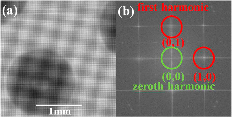
FIGURE 2. Raw image obtained in the experiment and 2D Fourier transform. (A) Raw image from an X-ray 2D grating–based phase contrast imaging system (the X-ray source is operated at 25 kVp, the mesh-type grating period is 78 μm with area duty cycle 0.63, the source-to-grating distance is 0.75 m, and the grating-to-detector distance is 0.25 m). (B) 2D Fourier transform of (A). The zeroth harmonic is labeled in green, and the first harmonic is labeled in red in Figure 2B.

The absorption is retrieved from the zeroth harmonic. A suitable harmonic width should be chosen, and the region of the zeroth harmonic is separated from the original Fourier transform plane to create a new Fourier transform plane. The harmonic width should be chosen properly to make sure no overlapping region exists between the region of the zeroth harmonic and higher harmonics. Then, the inverse Fourier transform is adopted. The same procedure is used for images with sample and without sample for normalization. And the computational formula of the absorption could be expressed as follows:

$I_{abs}=-\ln \left(\frac{F^{-1}\left\{H_{\left(\mathrm{0,0}\right)}^s\right\}}{F^{-1}\left\{H_{\left(\mathrm{0,0}\right)}^r\right\}}\right).(10)$

Here, $H_{\left(\mathrm{0,0}\right)}^s$ represents the separated zeroth harmonic with sample and $H_{\left(\mathrm{0,0}\right)}^r$ represents the separated zeroth harmonic without sample.

The differential phase contrast is retrieved from the first harmonic. As shown in Figure 2B, four first harmonics including $H_{\left(\mathrm{0,1}\right)}$, $H_{\left(\mathrm{1,0}\right)}$, $H_{\left(0,-1\right)}$, and $H_{\left(-\mathrm{1,0}\right)}$ could be seen in the Fourier transform plane. According to the symmetry of the Fourier transform, information contained in $H_{\left(\mathrm{0,1}\right)}$ is the same as in $H_{\left(0,-1\right)}$ and information contained in $H_{\left(\mathrm{1,0}\right)}$ is the same as in $H_{\left(-\mathrm{1,0}\right)}$. Therefore, both $H_{\left(\mathrm{1,0}\right)}$ and $H_{\left(\mathrm{0,1}\right)}$ could be used to retrieve differential phase contrast. The area of the first harmonic is separated to create a new Fourier transform plane. Then, the inverse Fourier transform is adopted for the separated first harmonic with sample and without sample. The difference between the angle information of the inverse Fourier transform with sample and without sample is defined as the differential phase contrast $\left(\frac{\partial \Phi \left(x,y\right)}{\partial x}\right)$ and $\left(\frac{\partial \Phi \left(x,y\right)}{\partial y}\right)$, which could be expressed as follows:

$I_{dpc}=\arg \left(F^{-1}\left\{H_{\left(\mathrm{1,0}\right)}^s\right\}\right)-\arg \left(F^{-1}\left\{H_{\left(\mathrm{1,0}\right)}^r\right\}\right)\mathit{or}{I}_{dpc}=\arg \left(F^{-1}\left\{H_{\left(\mathrm{0,1}\right)}^s\right\}\right)-\arg \left(F^{-1}\left\{H_{\left(\mathrm{0,1}\right)}^r\right\}\right).(11)$

Here, $H_{\left(\mathrm{1,0}\right)}^s$ and $H_{\left(\mathrm{0,1}\right)}^s$ represent the separated first harmonic with sample, $H_{\left(\mathrm{1,0}\right)}^r$ and $H_{\left(\mathrm{0,1}\right)}^r$ represent the separated first harmonic without sample, $\arg \left(\right)$ is the angle of the complex, and $\Phi \left(x,y\right)$ denotes the phase of the sample. Usually, the differential phase contrast could be obtained by choosing any one of these two first harmonics. And the phase image could be retrieved via integration along the axis. However, phase images obtained via single integration suffer from serious artifacts. Kottler et al. put forward an algorithm which uses both first harmonics to obtain good quality and artifact-free phase images [25]. And this algorithm is particularly appropriate for 2D grating–based imaging systems as the differential phase contrast of the two vertical directions can be obtained simultaneously.

The dark-field contains both the information of the zeroth harmonic and the first harmonic. According to the definition of the dark-field, it is the ratio between the visibility of the sample and of the background. The visibility is calculated via the ratio between the first harmonic and the zeroth harmonic. The first harmonic could also be chosen as $H_{\left(\mathrm{1,0}\right)}$ or $H_{\left(\mathrm{0,1}\right)}$. And the computational formula of the dark-field is given by the following equation:

$I_{df}=-\ln \left(\frac{F^{-1}\left\{H_{\left(\mathrm{1,0}\right)}^s\right\}·F^{-1}\left\{H_{\left(\mathrm{0,0}\right)}^r\right\}}{F^{-1}\left\{H_{\left(\mathrm{1,0}\right)}^r\right\}·F^{-1}\left\{H_{\left(\mathrm{0,0}\right)}^s\right\}}\right)or{I}_{df}=-\ln \left(\frac{F^{-1}\left\{H_{\left(\mathrm{0,1}\right)}^s\right\}·F^{-1}\left\{H_{\left(\mathrm{0,0}\right)}^r\right\}}{F^{-1}\left\{H_{\left(\mathrm{0,1}\right)}^r\right\}·F^{-1}\left\{H_{\left(\mathrm{0,0}\right)}^s\right\}}\right).(12)$

Simulation Results

The simulation is conducted according to the theory above. In order to simplify the situation, the X-ray source is simulated as a coherent unit-amplitude plane wave. Also, it is considered as a parallel light beam. In that case, the magnification of the sample is ignored. The wavelength of the X-ray is chosen as 0.155 nm. The sample in the 2D grating–based phase contrast imaging system is chosen as a resolution test chart which would be beneficial for further research on factors affecting the spatial resolution. As phase contrast studies are normally performed on weak-absorbing samples, PMMA is chosen as the material of the sample. The thickness of the resolution test chart is chosen as 200 μm. Figure 3 shows the transmittance image of this chart, which contains several lines at four different directions. The width of the lines ranges from 51.6 to 6.4 μm and is labeled in the figure. Considering the difficulty in the grating manufacture in reality, the mesh-type 2D ideal $\frac{\pi }{2}$ phase grating with an area duty cycle of 0.25 is chosen as the 2D grating in the simulation. The period of the mesh is set as 12.8 μm. The source-to-grating distance is 0.5 m. In order to obtain optimal fringe visibility, the grating-to-detector distance is set as 1.5855 m, which is the second Talbot distance of this grating. The grating-to-sample distance is 0.4756 m. And the sample-to-detector distance is 1.1099 m. The field of view of the simulated detector is $1638.4\mu m\times 1638.4\mu m$ with the pixel size of $1.6\mu m\times 1.6\mu m$. Considering the pixel size of the simulated detector, it is assumed that the MTF decreases to 0.1 when the spatial frequency comes to 312.5 lp/mm. Then, the spatial frequency constant is set as 213.9 lp/mm, and the device constant is set as 2.2. Normally, distributed random noise is added directly into the intensity images received by the detector with standard deviation $\sigma =3$ and mean value $\mu =0$. According to our calculation, the sampling window in the frequency domain in this simulation ($u$ and $v$) is in the frequency range for which the transfer function causes no aliasing error [26]. Therefore, the angular spectrum algorithm is appropriate for this simulation.

FIGURE 3

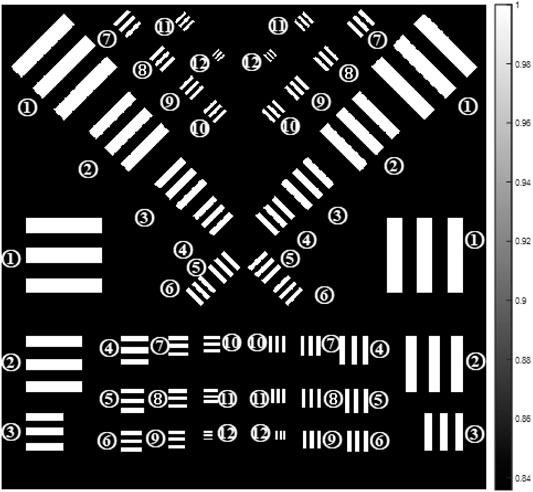
FIGURE 3. Resolution test chart (the width of the lines is ①51.2, ②38.4, ③25.6, ④19.2, ⑤16, ⑥14.4, ⑦13.6, ⑧12.8, ⑨12, ⑩11.2, ⑪9.6, and ⑫6.4 μm).

In this simulation, the resolution is evaluated without dose limit in order to ignore the influence of SNR, which is caused by limited amount of photons. And the resolution at different simulation conditions is compared via the minimum detectable line width of the resolution test chart. The minimum detectable line width at one single direction is evaluated via the intensity line profiles vertical to the three parallel lines at different line widths. If three obvious peaks could be seen in the profile of absorption and phase, then it indicates that these lines could be resolved. As for the dark-field images, there should be six obvious peaks in the profile of three parallel lines. The width of smallest resolved parallel lines is defined as the minimum detectable line width. In the following, the minimum detectable line width in absorption is determined from the calculated absorption results and the width in phase is evaluated from the integrated phase map via the method mentioned in [22]. The resolution of dark-field images is evaluated from the retrieved results in both x- and y-directions.

The simulation is conducted based on parameters given in the first paragraph of this section. Figure 4A presents the raw image obtained from the detector. The mesh and the resolution test chart could be clearly observed. And Figure 4B shows the 2D Fourier transform of Figure 4A, which is also shown in the logarithmic scale. One zeroth harmonic and four first harmonics could be seen on the Fourier transform plane. Three images including absorption, differential phase contrast, and dark-field are displayed in Figures 4C–G, respectively. And the retrieved phase image via the method mentioned in [22] is shown in Figure 4H. It can be inferred from Figures 4C, H that the minimum detectable line width is 12 μm in 0°/90° directions while 13.6 μm in 45°/135° directions. As for the phase, the minimum detectable line width is 11.2 μm in all four directions. The width is 13.6 μm in 0°/90° directions and 12.8 μm in 45°/135° directions for dark-field images.

FIGURE 4

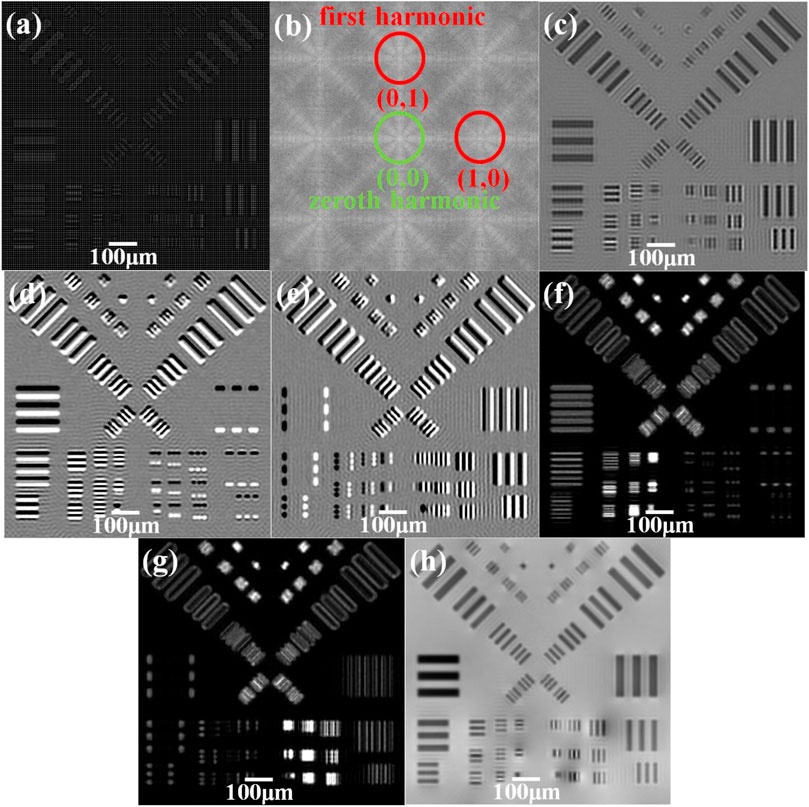
FIGURE 4. Images obtained from the simulation. (A) Raw image obtained on the detector plane. (B) 2D Fourier transform of raw image (A). (C) Retrieved absorption. (D) Retrieved differential phase contrast in the y-direction. (E) Retrieved differential phase contrast in the x-direction. (F) Retrieved dark-field in the y-direction. (G) Retrieved dark-field in the x-direction. (H) Retrieved phase.

There are quantities of variables in the 2D grating–based phase contrast imaging system. According to our selection, factors including the location of the sample, the period of 2D grating, the area duty cycle of the mesh, the shape of the mesh, and the width of harmonics in the spatial harmonic method are considered in this simulation.

The Location of the Sample

As shown in Figure 1A, the sample in our system is placed between the 2D grating and the detector. In order to explore the influence brought by the sample’s location, the grating-to-sample distance is set as 0.1586, 0.4757, 0.7928, and 1.1099 m, respectively. However, other parameters remain unchanged. The simulation results show that the minimum detectable line width of this resolution test chart in absorption, phase, and dark-field differs as the sample’s location changes, which is presented in Figures 5A–C. It could be concluded that the resolution improves as the distance between the grating and the sample increases. In order to verify our conclusion, the 1D differential phase contrast result of the 19.2 μm 45° lines in this resolution test chart is shown in Figure 5D. It could be seen that the resolution improves monotonously as the distance increases. At the same time, the contrast decreases as the distance increases. In short, high resolution and low contrast could be obtained when the sample is close to the detector, and vice versa.

FIGURE 5

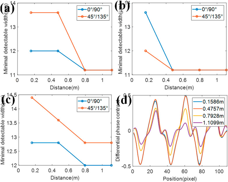
FIGURE 5. Simulation results on the location of the sample. The minimum detectable width at different distances in (A) absorption, (B) phase, and (C) dark-field. (D) 1D differential phase contrast result of the 19.2 μm 45° lines in this resolution test chart at different grating-to-sample distances.

The Period of the Mesh

In order to research how the period of 2D grating would affect the resolution of absorption, phase, and dark-field, meshes with a period of 9.6, 12.8, 19.2, 25.6, and 38.4 μm are chosen in this simulation. And all the other parameters remain the same. Figure 6A shows the simulation result in absorption, Figure 6B is the result in phase, and Figure 6C is the result in dark-field. The reason why the curve is not linear is the finite number of line widths chosen in our resolution testing chart. Also, the resolution differs at different directions in phase. The minimum detectable line widths in absorption, phase, and dark-field increase monotonously, with the increase in the period of the mesh. In order to achieve high resolution, a smaller grating period is preferred in the system.

FIGURE 6

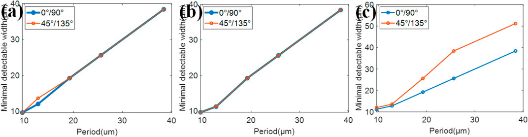
FIGURE 6. The minimum detectable width for different 2D grating periods in (A) absorption, (B) phase, and (C) dark-field.

The Area Duty Cycle of the Mesh

The area duty cycle determines the area of the transparent region when the period of mesh is fixed. In this simulation, the area duty cycle is chosen as 0.0625, 0.140625, 0.25, 0.390625, and 0.5625. And other parameters are the same as the previous ones. The minimum detectable line width of our resolution test chart is presented in Figures 7A–C. It could be concluded that the resolution in absorption gets worse when the area duty cycle increases. As for the phase and dark-field, when the area duty cycle is higher than 0.3925, the resolution gets worse as the area duty cycle increases. Meanwhile, as the duty cycle is lower than 0.3925, the resolution changes a little with the area duty ratio. Combining with the results obtained from the period of the mesh, it could be concluded that a small area of the transparent region does not always lead to the improvement of the spatial resolution. Also, a 1D differential phase contrast result of the 19.2 μm 45° lines in this resolution test chart is shown in Figure 7D. It is clear that the lower duty cycle would result in a higher contrast when the area duty cycle is below 0.3925. Meanwhile, considering the full width at half maximum (FWHM), the area duty cycle of 0.25 is more appropriate for higher resolution in our simulation.

FIGURE 7

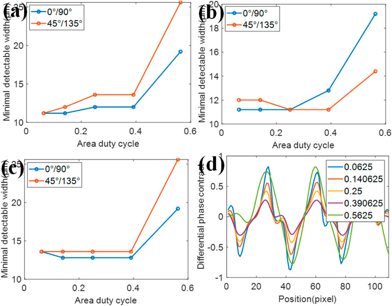
FIGURE 7. Simulation results on the area duty cycle of the mesh. The minimum detectable width for different 2D grating area duty cycles in (A) absorption, (B) phase, and (C) dark-field. (D) 1D differential phase result of the 19.2 μm 45° lines in this resolution test chart at different area duty cycles.

The Shape of the Mesh

Normally, the shape of the mesh is chosen as square, which means the period of grating on both x and y axes is the same. In this section, three different shapes of mesh (rectangle, parallelogram, and circle) are chosen for the imaging system, and these meshes are shown in Figure 8. The area duty cycle of rectangle and parallelogram meshes is set as 0.25, and that of the circle mesh is 0.2. All the other parameters remain the same. The simulation results are listed in Table 1 (for absorption), Table 2 (for phase), and Table 3 (for dark-field). From Figure 8, it could be seen that the period of gratings in two different directions differs. And the minimum detectable line width is affected by the larger one. In other words, even though the period of the grating in one direction is fabricated as extremely small, the spatial resolution could not be improved due to the limitation of the larger period one. As for circle-type gratings, it seems that their performance in absorption and dark-field is little worse than that of the square ones, and there is no difference in phase. Therefore, considering manufacturing costs, it is better to choose square as the shape of the mesh as the periods of gratings in two different directions are the same.

FIGURE 8

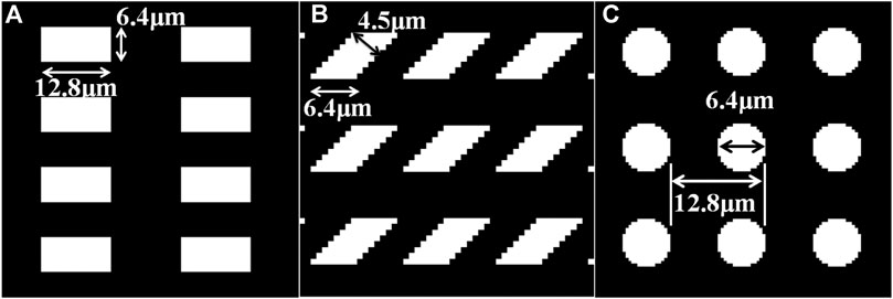
FIGURE 8. Three different shapes of mesh. (A) Rectangle type. (B) Parallelogram type. (C) Circle type.

TABLE 1

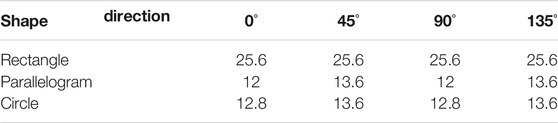
TABLE 1. Simulation results of the minimum detectable line width of our resolution test chart at different directions for absorption (μm).

TABLE 2

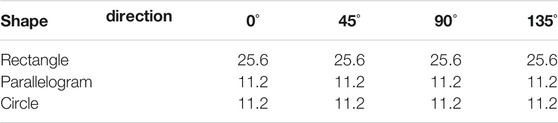
TABLE 2. Simulation results of the minimum detectable line width of our resolution test chart at different directions for phase (μm).

TABLE 3

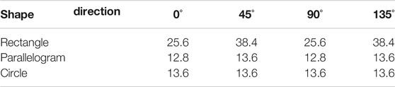
TABLE 3. Simulation results of the minimum detectable line width of our resolution test chart at different directions for dark-field (μm).

The Width of Harmonics in the Spatial Harmonic Method

Not only do optical elements in the 2D grating system would influence the spatial resolution of retrieved images, but also parameters in the retrieval method do affect the resolution. Here, we define the maximum width where there is no overlapping area between the zeroth harmonic and the first harmonic as $w_0$. Then, the width in this simulation is set as $0.4w_0$, $0.6w_0$, $0.8w_0$, and $w_0$, separately. The system parameters are the same as the conditions mentioned in the first paragraph of Simulation Results. The results of the minimum detectable width in absorption, phase, and dark-field are presented in Figures 9A–C. It could be concluded that a larger width of harmonics would result in a higher resolution in absorption, phase, and dark-field. This is because a larger width would contain more detailed information. Therefore, images would become more distinct due to the larger area of the frequency region. However, the width of harmonics could not increase unrestrictedly, which means there should be no overlapping area between each harmonic region. Otherwise, the signal aliasing problem would occur and images (absorption, phase, and dark-field) cannot be separated completely. In order to avoid signal aliasing problems, research toward removing unwanted harmonics would be useful for increasing the spatial resolution in the spatial harmonic method.

FIGURE 9

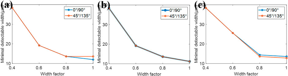
FIGURE 9. Simulation results on the width of harmonics in the spatial harmonic method. The minimum detectable width for different widths of harmonics in (A) absorption, (B) phase, and (C) dark-field.

Discussion

In conclusion to our simulation, the location of the sample, the period of 2D grating, the area duty cycle of the mesh, the shape of the mesh, and the width of harmonics in the spatial harmonic method all contribute to the spatial resolution. In order to achieve a higher resolution in three kinds of images, a larger distance between the sample and the grating is preferred. As for the grating period, it is well known that a smaller period of 2D grating results in a better resolution. However, the fabrication of a small period grating is now limited by micro- and nano-processing technology. In our simulation, 0.25 is the best area duty cycle in our experiment condition. When the other system parameters are set at different values, the best area duty cycle may change. The shape of the mesh is recommended as the square type, as the spatial resolution is restricted by the larger period of two different directions. In order to obtain a higher resolution, a larger width of harmonics is preferred. However, in order to avoid the signal aliasing problem caused by the overlapping area of harmonics, removal of unwanted harmonics would be beneficial to obtain a larger area of the harmonic region. As the real 2D grating–based X-ray phase contrast imaging system is much complicated, there exist other factors affecting the spatial resolution which we may ignore.

Besides the research on factors affecting spatial resolution, we also find limitation on the grating-to-detector distance in the spatial harmonic method for a totally or partially coherent X-ray source. Simulations are carried out by changing the grating-to-detector distance. The X-ray wavelength is also set as 0.155 nm. The period of the 2D absorb mesh is 12.8 μm with the area duty cycle of 0.25. The source-to-grating distance is set as 0.8 m. The grating-to-detector distance is set as 0.529, 0.634, 0.951, and 1.057 m. No samples are placed in the system. Figure 10 shows raw images obtained from the detector. Different periodic patterns could be observed at different distances in Figure 10B–D, which is caused by Fresnel diffraction. By applying 2D Fourier transform on these images, both the zeroth harmonic and the first harmonic could be acquired. And then absorption, differential phase contrast, and dark-field could be retrieved via the Fourier transform method at these distances. However, it is clear that no periodic structure could be found in Figure 10A. Meanwhile, only the zeroth harmonic could be seen in the Fourier space, which results in the failure to retrieve differential phase contrast and dark-field images. This phenomenon is caused due to the Talbot effect. Not only the 2D absorb mesh-type grating but also all 2D gratings do have the distance limitation according to our further simulation. And the limited distance is not the same. Moreover, this limited distance changes when the area duty cycle of the 2D grating varies. It seems difficult to give an accurate expression of this limited distance as it changes with both the area duty cycle and type of the 2D grating. It is recommended to avoid setting the distance between the 2D grating and the detector as the limited distance or around it when building the system.

FIGURE 10

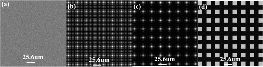
FIGURE 10. Raw images obtained from the detector. The grating-to-detector distance is (A) 0.529 m, (B) 0.634 m, (C) 0.951 m, and (D) 1.057 m.

This simulation is suitable for 2D grating–based X-ray phase contrast imaging in which the X-ray source is completely or partially coherent as a synchrotron radiation source, microfocus source, or traditional X-ray tube with a source grating. It is not appropriate to simulate incoherent X-ray source–based imaging systems with scalar diffraction theory and the operator theory of imaging due to their difficulty in establishing the diffraction model and higher calculation. And simulations based on the Monte Carlo algorithm are preferred for these systems. The conclusions we drew are based on the simulation merely. The experimental conditions are relatively complex, and there are many unknown factors left unaccounted for. Therefore, further study could be carried out in the experiment to determine factors which may influence the spatial resolution of absorption and phase contrast.

Conclusion

In this paper, we successfully simulated raw images obtained from a 2D grating–based phase contrast imaging system. Absorption, differential phase contrast, and dark-field are retrieved from a single raw image via the Fourier transform method. The factors affecting the spatial resolution of absorption and phase contrast were studied. The location of the sample, the period of 2D grating, the area duty cycle of the 2D grating, and the width of harmonics in the spatial harmonic method play vital roles in determining the spatial resolution. Meanwhile, the shape of the 2D grating should also be chosen properly. It is also worth noting that the spatial resolution differs at different directions in both absorption and phase contrast under certain conditions. Besides the simulation toward the spatial resolution, distance limitation in the spatial harmonic method is also investigated. The grating-to-detector distance should not be set with certain values, or the first harmonic would disappear in the spatial harmonic method, which causes the failure to obtain differential phase contrast and dark-field images via the Fourier transform method. The research on the spatial resolution and the distance limitation would be instructive for building a 2D grating–based phase contrast imaging system. So, our work would be beneficial for further development in high-resolution X-ray biological microscopy.

Data Availability Statement

The original contributions presented in the study are included in the article/supplementary Material, and further inquiries can be directed to the corresponding authors.

Author Contributions

ST and XL contributed to conception and design of the study. XH and CK organized the database. ST and CH performed statistical analysis. ST wrote the first draft of the manuscript. CH and XH wrote sections of the manuscript. XH, CK, and XL contributed to funding acquisition. All authors contributed to manuscript revision and read and approved the submitted version.

Funding

This research was funded by the National Natural Science Foundation of China (61827825 and 61735017), Key Research and Development Program of Zhejiang Province (2020C01116), Fundamental Research Funds for the Central Universities (2019XZZX003-06 and K20200132), and Zhejiang Lab (2018EB0ZX01 and 2020MC0AE01).

Conflict of Interest

The authors declare that the research was conducted in the absence of any commercial or financial relationships that could be construed as a potential conflict of interest.

References

1. Bonse U, Hart M. An X‐ray Interferometer. Appl Phys Lett (1965) 6(8):155–6. doi:10.1063/1.1754212

CrossRef Full Text | Google Scholar

2. Pfeiffer F, Bech M, Bunk O, Kraft P, Eikenberry EF, Brönnimann C, et al. Hard-X-ray Dark-Field Imaging Using a Grating Interferometer. Nat Mater (2008) 7(2):134–7. doi:10.1038/nmat2096

PubMed Abstract | CrossRef Full Text | Google Scholar

3. Momose A. Recent Advances in X-ray Phase Imaging. Jpn J Appl Phys (2005) 44(9A):6355–67. doi:10.1143/jjap.44.6355

CrossRef Full Text | Google Scholar

4. David C, Nöhammer B, Solak HH, Ziegler E. Differential X-ray Phase Contrast Imaging Using a Shearing Interferometer. Appl Phys Lett (2002) 81(17):3287–9. doi:10.1063/1.1516611

CrossRef Full Text | Google Scholar

5. Momose A, Kawamoto S, Koyama I, Hamaishi Y, Taikai K, Suzuki Y. Demonstration of X-Ray Talbot Interferometry. Jpn J Appl Phys Part 2 (Letters (2003) 42(7B):L866–L868. doi:10.1143/jjap.42.l866

CrossRef Full Text | Google Scholar

6. Iwata K. X-ray Shearing Interferometer and Generalized Grating Imaging. Appl Opt (2009) 48(5):886–92. doi:10.1364/ao.48.000886

PubMed Abstract | CrossRef Full Text | Google Scholar

7. Engelhardt M, Baumann J, Schuster M, Kottler C, Pfeiffer F, Bunk O, et al. High-resolution Differential Phase Contrast Imaging Using a Magnifying Projection Geometry with a Microfocus X-ray Source. Appl Phys Lett (2007) 90(22):224101. doi:10.1063/1.2743928

CrossRef Full Text | Google Scholar

8. Weitkamp T, David C, Kottler C, Bunk O, Pfeiffer F. Tomography with Grating Interferometers at Low-Brilliance Sources. Proc SPIE: Int Soc Opt Eng (2006) 6318:63180S.

Google Scholar

9. Pfeiffer F, Weitkamp T, Bunk O, David C. Phase Retrieval and Differential Phase-Contrast Imaging with Low-Brilliance X-ray Sources. Nat Phys (2006) 2(4):258–61. doi:10.1038/nphys265

CrossRef Full Text | Google Scholar

10. Kageyama M, Okajima K, Maesawa M, Nonoguchi M, Koike T, Noguchi M, et al. X-ray Phase-Imaging Scanner with Tiled Bent Gratings for Large-Field-Of-View Nondestructive Testing. NDT E Int (2019) 105:19–24. doi:10.1016/j.ndteint.2019.04.007

CrossRef Full Text | Google Scholar

11. Yoshioka H, Kadono Y, Kim YT, Oda H, Maruyama T, Akiyama Y, et al. Imaging Evaluation of the Cartilage in Rheumatoid Arthritis Patients with an X-ray Phase Imaging Apparatus Based on Talbot-Lau Interferometry. Sci Rep (2020) 10(1):6561. doi:10.1038/s41598-020-63155-9

PubMed Abstract | CrossRef Full Text | Google Scholar

12. Ludwig V, Seifert M, Hauke C, Hellbach K, Horn F, Pelzer G, et al. Exploration of Different X-ray Talbot-Lau Setups for Dark-Field Lung Imaging Examined in a Porcine Lung. Phys Med Biol (2019) 64(6):065013. doi:10.1088/1361-6560/ab051c

PubMed Abstract | CrossRef Full Text | Google Scholar

13. Beltran A, Paganin M, Pelliccia D. Phase-and-amplitude Recovery from a Single Phase-Contrast Image Using Partially Spatially Coherent X-ray Radiation. J Opt (2018) 20(5):055605. doi:10.1088/2040-8986/aabbdd

CrossRef Full Text | Google Scholar

14. Wen H, Bennett EE, Hegedus MM, Carroll SC. Spatial Harmonic Imaging of X-ray Scattering-Initial Results. IEEE Trans Med Imaging (2008) 27(8):997–1002. doi:10.1109/tmi.2007.912393

PubMed Abstract | CrossRef Full Text | Google Scholar

15. Wen HH, Bennett EE, Kopace R, Stein AF, Pai V. Single-shot X-ray Differential Phase-Contrast and Diffraction Imaging Using Two-Dimensional Transmission Gratings. Opt Lett (2010) 35(12):1932–4. doi:10.1364/ol.35.001932

PubMed Abstract | CrossRef Full Text | Google Scholar

16. Itoh H, Nagai K, Sato G, Yamaguchi K, Nakamura T, Kondoh T, et al. Two-dimensional Grating-Based X-ray Phase-Contrast Imaging Using Fourier Transform Phase Retrieval. Opt express (2011) 19(4):3339–46. doi:10.1364/oe.19.003339

PubMed Abstract | CrossRef Full Text | Google Scholar

17. Jiang M, Wyatt CL, Wang G. X-Ray Phase-Contrast Imaging with Three 2D Gratings. Int J Biomed Imaging (2008) 2008(1):827152. doi:10.1155/2008/827152

CrossRef Full Text | Google Scholar

18. Rix KR, Dreier T, Shen T, Bech M. Super-resolution X-ray Phase-Contrast and Dark-Field Imaging with a Single 2D Grating and Electromagnetic Source Stepping. Phys Med Biol (2019) 64(16):165009. doi:10.1088/1361-6560/ab2ff5

PubMed Abstract | CrossRef Full Text | Google Scholar

19. Birnbacher L, Willner M, Velroyen A, Marschner M, Hipp A, Meiser J, et al. Experimental Realisation of High-Sensitivity Laboratory X-ray Grating-Based Phase-Contrast Computed Tomography. Sci Rep (2016) 6:24022. doi:10.1038/srep24022

PubMed Abstract | CrossRef Full Text | Google Scholar

20. Ji X, Zhang R, Li K, Chen GH. Is High Sensitivity Always Desirable for a Grating‐based Differential Phase Contrast Imaging System? Med Phys (2020) 47(3):1215–28. doi:10.1002/mp.13984

PubMed Abstract | CrossRef Full Text | Google Scholar

21. Fraiz W, Zhu P, Hu R, Gao K, Wu Z, Bao Y, et al. Signal-to-noise Ratio Comparison of Angular Signal Radiography and Phase Stepping Method. Chin Phys B (2017) 26(12):120601. doi:10.1088/1674-1056/26/12/120601

CrossRef Full Text | Google Scholar

22. Takano H, Wu Y, Momose A. Development of Full-Field X-ray Phase-Tomographic Microscope Based on Laboratory X-ray Source. In: SPIE Conference on Developments in X-Ray Tomography XI, San Diego, CA, August 8–10, 2017 (Washington, DC:SPIE), 10391 (2017). 1039110. doi:10.1117/12.2273534

CrossRef Full Text | Google Scholar

23. Zanette I, David C, Rutishauser S, Weitkamp T. 2D Grating Simulation for X-ray Phase-Contrast and Dark-Field Imaging with a Talbot Interferometer. In: 20th International Congress on X-Ray Optics and Microanalysis, Karlsruhe, Germany, September 15–18, 2009, 1221 (2010). 73. doi:10.1063/1.3399260

CrossRef Full Text | Google Scholar

24. Born M, Wolf E. Principles of Optics. 7th ed. Cambridge, United Kingdom: Cambridge University Express (1999).

25. Kottler C, David C, Pfeiffer F, Bunk O. A Two-Directional Approach for Grating Based Differential Phase Contrast Imaging Using Hard X-Rays. Opt Express (2007) 15(3):1175–81. doi:10.1364/oe.15.001175

PubMed Abstract | CrossRef Full Text | Google Scholar

26. Matsushima K, Shimobaba T. Band-Limited Angular Spectrum Method for Numerical Simulation of Free-Space Propagation in Far and Near Fields. Opt Express (2009) 17(22):19662–73. doi:10.1364/oe.17.019662

PubMed Abstract | CrossRef Full Text | Google Scholar