Gaussian Local Phase Approximation in a Cylindrical Tissue Model

In NMR or MRI, the measured signal is a function of the accumulated magnetization phase inside the measurement voxel, which itself depends on microstructural tissue parameters. Usually the phase distribution is assumed to be Gaussian and higher-order moments are neglected. Under this assumption, only the x-component of the total magnetization can be described correctly, and information about the local magnetization and the y-component of the total magnetization is lost. The Gaussian Local Phase (GLP) approximation overcomes these limitations by considering the distribution of the local phase in terms of a cumulant expansion. We derive the cumulants for a cylindrical muscle tissue model and show that an efficient numerical implementation of these terms is possible by writing their definitions as matrix differential equations. We demonstrate that the GLP approximation with two cumulants included has a better fit to the true magnetization than all the other options considered. It is able to capture both oscillatory and dampening behavior for different diffusion strengths. In addition, the introduced method can possibly be extended for models for which no explicit analytical solution for the magnetization behavior exists, such as spherical magnetic perturbers.

1. Introduction

The extraction of parameters describing the tissue architecture from MRI measurements is dependent on the correct description of susceptibility and diffusion effects during spin dephasing. While analytical solutions of the underlying Bloch-Torrey equation [1, 2] are possible only for simple geometries, approximate methods are often sufficient in practice [3]. The important Gaussian phase approximation, introduced by Hahn [4] to describe the signal behavior inside a linear and uniform magnetic field gradient, assumes a Gaussian distribution of the accumulated spin phases. Recently, the Gaussian Local Phase (GLP) approximation was introduced [5]. Instead of the cumulative phase distribution inside a measurement voxel, the local phase distribution is expanded in a cumulant expansion and the integration over the voxel carried out afterward. Herein, we consider the case of a muscle tissue model which consists of a blood vessel surrounded by a cylindrical dephasing domain [6]. Due to the shape of this domain, the resulting diffusion propagator takes a rather complex form. The calculation of the magnetization time evolution is then dependent on zeros of cross products of Bessel functions, making it impractical to use [3, 7]. To overcome this limitation, we present a convenient calculation method for the GLP moments based on a finite-difference approximation of the cylindrical Laplace operator. This permits formulating the first and second moments of the phase distribution as closed-form matrix exponentials, which are easy to implement numerically. We compare the new method to results obtained from integrating over the analytical diffusion propagator and to the numerically exact results from a finite-element simulation [8–11].

The manuscript is structured as follows. In section 2.1, we define the muscle tissue model and show the diffusion propagator. Integrating over products of the diffusion propagator and the local Larmor frequency allows the analytical calculation of the phase moments, as shown in sections 2.2 and 2.3. In section 3.1, the finite-difference scheme is introduced and used to write the governing differential equations as vector differential equations. The solutions are rather straightforward and result in the vector forms of the phase moments. These are then used to calculate the local magnetization in section 3.2 and the total magnetization in section 3.3. Finally, the introduced methods are compared to previously known solutions described in section 3.4. In Appendix A, the cumulant expansion and its statistical properties are reviewed. Alternative expressions for the cumulant functions are given in Appendix B, and a spectral expansion of the Laplace operator is shown in Appendix C. As the discretized Laplace operator is singular, its group inverse has to be used. This group inverse can be expressed in terms of simple functions, as detailed in Appendix D.

2. Methods

2.1. Model and Diffusion Process

We considered a muscle tissue model which consists of a radially-symmetric dephasing domain parallel to the z-axis and bounded at R_C and R_D, as shown in Figure 1. As the model is invariant along the z-axis, it is sufficient to parametrize the dephasing domain in terms of polar coordinates (r, ϕ): $\overrightarrow{r}=(r,\varphi )\in \left[R_{\text{C}},R_{\text{D}}\right]\times [0,2\pi )$. The inner cylinder with radius R_C > 0 represents a blood-filled vessel and therefore creates a spatially varying Larmor frequency [12]

$\begin{array}{ll}\omega (r,\varphi )=\delta \omega R_{\text{C}}^2\frac{cos(2\varphi )}{r^2},& (1)\end{array}$

with δω being the characteristic frequency shift at the vessel surface, which is proportional to the susceptibility difference between vessel and dephasing domain. The Larmor frequency is visualized in the upper part of Figure 1. In the following derivations, we assume without loss of generality that the external magnetic field is orthogonal to the cylinder axis. In the case of a different angle θ ≠ π between the cylinder axis and the magnetic field, δω is modified by a factor of sin²(θ) (see Equation (7) in [12]). The geometry can be described by the volume ratio

$\begin{array}{ll}\eta =\frac{R_{\text{C}}^2}{R_{\text{D}}^2}.& (2)\end{array}$

FIGURE 1

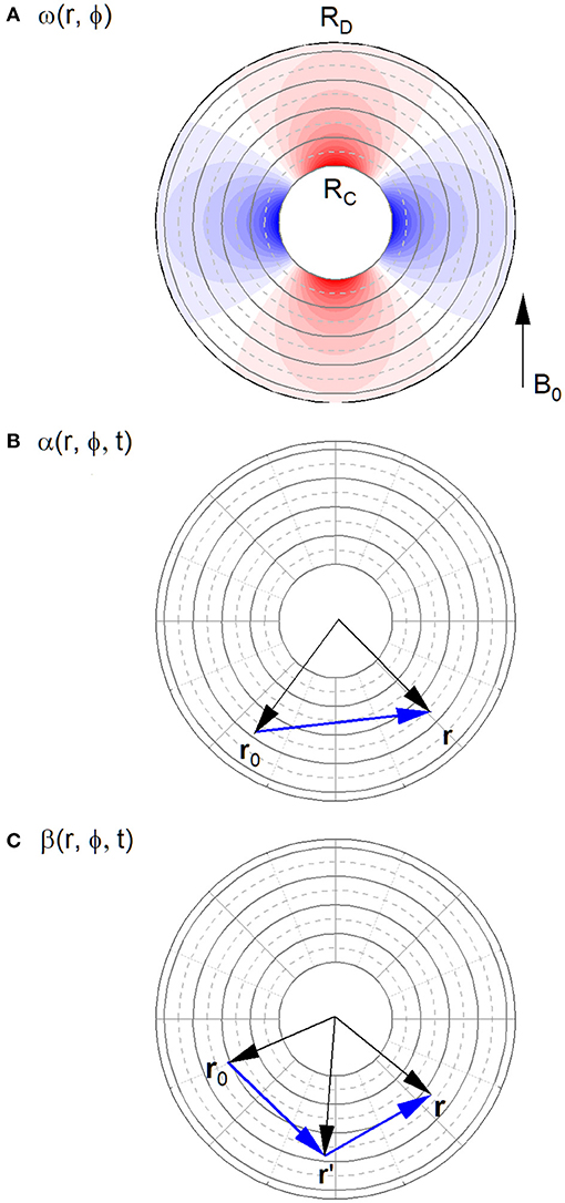
Figure 1. Larmor frequency and phase distribution moments. (A) Larmor frequency in the dephasing domain. The red and blue regions correspond to positive and negative values of ω(r, ϕ). The external magnetic field B₀ is indicated by a black arrow. (B) First moment of the phase distribution, corresponding to taking into account one previous location. (C) Second moment of the phase distribution, corresponding to taking into account two previous locations.

Inside the dephasing domain, spin-1/2 particles can diffuse freely with an isotropic and spatially homogeneous diffusion constant D > 0. The characteristic diffusion time τ for this model is then given by

$\begin{array}{ll}\tau =\frac{R_{\text{C}}^2}{D}.& (3)\end{array}$

As the muscle model is assumed to be surrounded by identical tissue cylinders, the crossing-over of particles into the domain of neighboring capillaries can be considered by introducing reflecting Neumann boundary conditions at R_D. The boundary condition at the interior border R_C is dependent on the assumed permeability of the vessel wall: negligible permeability corresponds to reflecting boundary conditions, while non-zero vessel permeability can be taken into account by choosing Robin-type boundary conditions, as shown, for example, in Equation (7) in Ziener et al. [13]. The Gaussian diffusion process is described by the propagator $p(\overrightarrow{r},{\overrightarrow{r}}_0,t)$, which is the solution of the diffusion equation

$\begin{array}{ll}\frac{\partial p(\overrightarrow{r},{\overrightarrow{r}}_0,t)}{\partial t}=D\Delta p(\overrightarrow{r},{\overrightarrow{r}}_0,t),& (4)\end{array}$

with the initial condition

$\begin{array}{ll}p(\overrightarrow{r},{\overrightarrow{r}}_0,t=0)=\delta (\overrightarrow{r}-{\overrightarrow{r}}_0).& (5)\end{array}$

Using the definition of the Laplace operator in cylinder coordinates

$\begin{array}{ll}\Delta ={\Delta }_r+\frac{1}{r^2}{\Delta }_{\varphi }=\frac{{\partial }^2}{\partial r^2}+\frac{1}{r}\frac{\partial }{\partial r}+\frac{1}{r^2}\frac{{\partial }^2}{\partial {\varphi }^2}& (6)\end{array}$

the solution to the diffusion equation can be written as

$\begin{array}{ll}p(\overrightarrow{r},{\overrightarrow{r}}_0,\xi )={\text{e}}^{D\xi \left[{\Delta }_r+\frac{1}{r^2}{\Delta }_{\varphi }\right]}\delta (\overrightarrow{r}-{\overrightarrow{r}}_0).& (7)\end{array}$

Due to the unboundedness of the radial Laplace operator Δ_r on the real line [0, ∞] under the L₂-norm, the radial part of the operator exponential cannot be readily written as a Taylor series. It can, however, be expanded in terms of eigenfunctions of the Laplace operator [14–18]. The propagator can then be written in the classical form [19, 20]:

$\begin{array}{l}p(r,\varphi ,r_0,{\varphi }_0,\xi )=\frac{1}{2\pi R_{\text{C}}^2}\times \\ {\displaystyle \sum _{n=1}^{\infty }}{\displaystyle \sum _{\nu =0}^{\infty }}\frac{{\text{e}}^{-{\lambda }_{n,\nu }^2\frac{D\xi }{R_{\text{C}}^2}}}{N_{n,\nu }}{\Phi }_{n,\nu }(r){\Phi }_{n,\nu }(r_0)\left[2-{\delta }_{\nu ,0}\right]cos(\nu \left[\varphi -{\varphi }_0\right]),& (8)\end{array}$

where the radial eigenfunctions Φ_n,ν(r) and the eigenvalues λ_n,ν obey the cylindrical Bessel differential equation

$\begin{array}{ll}\left[{\Delta }_r-\frac{{\nu }^2}{r^2}\right]{\Phi }_{n,\nu }(r)=-\frac{{\lambda }_{n,\nu }^2}{R_{\text{C}}^2}{\Phi }_{n,\nu }(r)& (9)\end{array}$

with the radial part of two-dimensional Laplace operator Δ_r given in Equation (6) inside an annular ring R_C ≤ r ≤ R_D. Reflecting boundary conditions at r = R_C and r = R_D are assumed:

$\begin{array}{ll}\frac{\partial }{\partial r}{\Phi }_{n,\nu }(r){|}_{r=R_{\text{C}}}=0& (10)\end{array}$

$\begin{array}{ll}\frac{\partial }{\partial r}{\Phi }_{n,\nu }(r){|}_{r=R_{\text{D}}}=0.& (11)\end{array}$

The appropriate eigenfunctions that obey the reflecting boundary conditions (10) at r = R_C are linear combinations of cylindrical Bessel functions J_ν and Y_ν of order ν and of the first and second kind, respectively:

$\begin{array}{l}{\Phi }_{n,\nu }\left(r\right)=\\ \{\begin{array}{ll}1& \text{for }n=1,\nu =0,\\ J_1\left({\lambda }_{n,0}\right)Y_0\left({\lambda }_{n,0}\frac{r}{R_{\text{C}}}\right)-Y_1\left({\lambda }_{n,0}\right)J_0\left({\lambda }_{n,0}\frac{r}{R_{\text{C}}}\right)& \text{for }n\ge 2,\nu =0,\\ Y_{\nu }^{\prime }\left({\lambda }_{n,\nu }\right)J_{\nu }\left({\lambda }_{n,\nu }\frac{r}{R_{\text{C}}}\right)-J_{\nu }^{\prime }\left({\lambda }_{n,\nu }\right)Y_{\nu }\left({\lambda }_{n,\nu }\frac{r}{R_{\text{C}}}\right)& \text{for }n\ge 1,\nu \ge 1,\end{array}& (12)\end{array}$

for all other combinations of indices. These eigenfunctions obey the orthogonality relation

$\begin{array}{ll}\frac{1}{R_C^2}{\displaystyle \underset{R_C}{\overset{R_D}{\int }}}\text{d}rr{\Phi }_{n,\nu }(r){\Phi }_{n^{\prime },\nu }(r)=N_{n,\nu }{\delta }_{n{n}^{\prime }}& (13)\end{array}$

with the normalization constants

$\begin{array}{l}{N}_{n,\nu }=\\ \{\begin{array}{ll}\frac{1-\eta }{2\eta }& \text{for }n=1,\nu =0\\ \frac{2}{{\pi }^2{\lambda }_{n,0}^2}\left[{\left[\frac{J_1({\lambda }_{n,0})}{J_1(\frac{{\lambda }_{n,0}}{\sqrt{\eta }})}\right]}^2-1\right]& \text{for }n\ge 2,\nu =0\\ \frac{2}{{\pi }^2{\lambda }_{n,\nu }^2}\left[\left[1-\frac{\eta {\nu }^2}{{\lambda }_{n,\nu }^2}\right]{\left[\frac{J_{\nu }^{\prime }({\lambda }_{n,\nu })}{J_{\nu }^{\prime }(\frac{{\lambda }_{n,\nu }}{\sqrt{\eta }})}\right]}^2-1+\frac{{\nu }^2}{{\lambda }_{n,\nu }^2}\right]& \text{for }n\ge 1,\nu \ge 1\end{array}& (14)\end{array}$

The lowest eigenvalue takes the value zero, while all other eigenvalues λ_n,ν can be obtained by introducing the eigenfunctions from Equation (12) into the reflecting boundary conditions (11) at r = R_D as solutions of a transcendental equation

$\begin{array}{lll}{\lambda }_{1,0}=0& \text{for\hspace{1em}}n=1,\nu =0,& (15)\end{array}$

$\begin{array}{lll}{Y}_1({\lambda }_{n,0})J_1\left(\frac{{\lambda }_{n,0}}{\sqrt{\eta }}\right)=J_1({\lambda }_{n,0})Y_1\left(\frac{{\lambda }_{n,0}}{\sqrt{\eta }}\right)& \text{for\hspace{1em}}n\ge 2,\nu =0,& (16)\end{array}$

$\begin{array}{lll}{Y}_{\nu }^{\prime }({\lambda }_{n,\nu })J_{\nu }^{\prime }\left(\frac{{\lambda }_{n,\nu }}{\sqrt{\eta }}\right)=J_{\nu }^{\prime }({\lambda }_{n,\nu })Y_{\nu }^{\prime }\left(\frac{{\lambda }_{n,\nu }}{\sqrt{\eta }}\right)& \text{for\hspace{1em}}n\ge 1,\nu \ge 1.& (17)\end{array}$

The eigenvalues can be calculated in Mathematica (Wolfram Research, Inc., Champaign, IL, United States) using the package BesselZeros. For ν = 0 and n ≥ 2 the correct command is

λ_n,0 = BesselJYJYZeros[1, 1/$\sqrt{\eta }$, n − 1][[n - 1]],

and for ν ≥ 1 and n ≥ 1, the command is

λ_n,ν = BesselJPrimeYPrimeJPrimeYPrimeZeros[ν, 1/$\sqrt{\eta }$, n][[n]].

Alternatively, the eigenvalues can be obtained as the eigenvalues of a discretized Laplace operator as demonstrated in Ziener et al. [21].

2.2. Moment Calculation

The signal generated during a NMR experiment can be calculated by approximating the local accumulated phase distribution by a cumulant expansion as detailed in Appendix A. Taking only the first cumulant into account, as seen in Equation (A7), the local magnetization can be written as

$\begin{array}{ll}{m}_I(\overrightarrow{r},t)=m_0(\overrightarrow{r}){\text{e}}^{\text{i}\alpha (\overrightarrow{r},t)},& (18)\end{array}$

which is further denoted as the first-order GLP approximation, with the first moment function denoted by $\alpha (\overrightarrow{r})$. For simplicity, the initial magnetization m₀(r) is from now on set to the constant m₀, corresponding to the voxel state immediately after application of the initial pulse. If both first and second cumulants are included, as seen in Equation (A8), this becomes

$\begin{array}{ll}{m}_{II}(\overrightarrow{r},t)=m_0{\text{e}}^{\text{i}\alpha (\overrightarrow{r},t)-\beta (\overrightarrow{r},t)+\frac{1}{2}{\left[\alpha (\overrightarrow{r},t)\right]}^2},& (19)\end{array}$

further denoted as second-order GLP approximation, with the second moment function denoted by $\beta (\overrightarrow{r},t)$. The real part of the local magnetization corresponds to the x-component of the transverse magnetization and the imaginary part to the y-component. Inserting $m_I(\overrightarrow{r},t)$ and $m_{II}(\overrightarrow{r},t)$ into the transverse Bloch-Torrey equation

$\begin{array}{ll}\frac{\partial m(\overrightarrow{r},t)}{\partial t}=\left[D\Delta -\text{i}\omega (\overrightarrow{r})\right]m(\overrightarrow{r},t)& (20)\end{array}$

and collecting real and imaginary terms leads to two inhomogeneous partial differential equations for the moment functions:

$\begin{array}{ll}\frac{\partial }{\partial t}\alpha (\overrightarrow{r},t)=D\Delta \alpha (\overrightarrow{r},t)-\omega (\overrightarrow{r}),& (21)\end{array}$

$\begin{array}{ll}\frac{\partial }{\partial t}\beta (\overrightarrow{r},t)=D\Delta \beta (\overrightarrow{r},t)-\omega (\overrightarrow{r})\alpha (\overrightarrow{r},t).& (22)\end{array}$

The initial conditions can be seen from the definitions in Equations (26) and (27):

$\begin{array}{ll}\alpha (\overrightarrow{r},0)=\beta (\overrightarrow{r},0)=0.& (23)\end{array}$

The boundary conditions on the moments similarly arise from the reflecting boundary conditions on $m(\overrightarrow{r},t)$ for both real and complex parts:

$\begin{array}{ll}\frac{\partial }{\partial r}\alpha (\overrightarrow{r},t){|}_{r=R_{\text{C}}}=\frac{\partial }{\partial r}\alpha (\overrightarrow{r},t){|}_{r=R_{\text{D}}}=0,& (24)\end{array}$

$\begin{array}{ll}\frac{\partial }{\partial r}\beta (\overrightarrow{r},t){|}_{r=R_{\text{C}}}=\frac{\partial }{\partial r}\beta (\overrightarrow{r},t){|}_{r=R_{\text{D}}}=0.& (25)\end{array}$

The solutions to the differential equations (21) and (22) are also given by integrals over products of the propagator and the Larmor frequency:

$\begin{array}{ll}\alpha (\overrightarrow{r},t)=-{\displaystyle \underset{0}{\overset{t}{\int }}}\text{d}\xi {\displaystyle \underset{V}{\int }}{\text{d}}^3{\overrightarrow{r}}_{0}p(\overrightarrow{r},{\overrightarrow{r}}_0,\xi )\omega ({\overrightarrow{r}}_0),& (26)\end{array}$

$\begin{array}{ll}\beta (\overrightarrow{r},t)={\displaystyle \underset{0}{\overset{t}{\int }}}\text{d}\eta {\displaystyle \underset{0}{\overset{t-\eta }{\int }}}\text{d}\xi {\displaystyle \underset{V}{\int }}{\text{d}}^3{\overrightarrow{r}}^{\prime }{\displaystyle \underset{V}{\int }}{\text{d}}^3{\overrightarrow{r}}_{0}p(\overrightarrow{r},{\overrightarrow{r}}^{\prime },\xi )\omega ({\overrightarrow{r}}^{\prime })p({\overrightarrow{r}}^{\prime },{\overrightarrow{r}}_0,\eta )\omega ({\overrightarrow{r}}_0),& (27)\end{array}$

where the spatial integrals go over the dephasing domain V. This relationship is visualized in the middle and lower subfigure of Figure 1. Here, the diffusion propagators take the form of ordinary functions, but later on they are used in a non-commutative operator form, in which case the specific ordering matters. The form presented here is valid in both cases.

Inserting the propagator from Equation (B3) into the definitions of the moment functions in Equations (26) and (27) and performing the angular integration yields an explicit expression for the angular dependence of the moments:

$\begin{array}{ll}\alpha (\overrightarrow{r},t)={\alpha }_2(r,t)cos(2\varphi ),& (28)\end{array}$

$\begin{array}{ll}\beta (\overrightarrow{r},t)={\beta }_0(r,t)+{\beta }_4(r,t)cos(4\varphi ),& (29)\end{array}$

with

$\begin{array}{ll}{\alpha }_2(r,t)=-\delta \omega {\displaystyle \underset{0}{\overset{t}{\int }}}\text{d}\xi {\text{e}}^{D\xi \left[{\Delta }_r-\frac{4}{r^2}\right]}\frac{R_{\text{C}}^2}{r^2}& (30)\end{array}$

$\begin{array}{ll}{\beta }_0(r,t)=\frac{3}{2}\delta {\omega }^2{\displaystyle \underset{0}{\overset{t}{\int }}}\text{d}\eta {\displaystyle \underset{0}{\overset{t-\eta }{\int }}}\text{d}\xi {\text{e}}^{D\xi {\Delta }_r}\frac{R_{\text{C}}^2}{r^2}{\text{e}}^{D\eta \left[{\Delta }_r-\frac{4}{r^2}\right]}\frac{R_{\text{C}}^2}{r^2},& (31)\end{array}$

$\begin{array}{ll}{\beta }_4(r,t)=\frac{1}{2}\delta {\omega }^2{\displaystyle \underset{0}{\overset{t}{\int }}}\text{d}\eta {\displaystyle \underset{0}{\overset{t-\eta }{\int }}}\text{d}\xi {\text{e}}^{D\xi \left[{\Delta }_r-\frac{16}{r^2}\right]}\frac{R_{\text{C}}^2}{r^2}{\text{e}}^{D\eta \left[{\Delta }_r-\frac{4}{r^2}\right]}\frac{R_{\text{C}}^2}{r^2}.& (32)\end{array}$

The angular decomposition directly leads to a system of three inhomogeneous partial differential equations for α₂(r, t), β₀(r, t), and β₄(r, t):

$\begin{array}{ll}\frac{\partial }{\partial t}{\alpha }_2(r,t)=D\left[{\Delta }_r-\frac{4}{r^2}\right]{\alpha }_2(r,t)-\delta \omega \frac{R_{\text{C}}^2}{r^2},& (33)\end{array}$

$\begin{array}{ll}\frac{\partial }{\partial t}{\beta }_0(r,t)=D{\Delta }_r{\beta }_0(r,t)-\frac{\delta \omega }{2}\frac{R_{\text{C}}^2}{r^2}{\alpha }_2(r,t),& (34)\end{array}$

$\begin{array}{ll}\frac{\partial }{\partial t}{\beta }_4(r,t)=D\left[{\Delta }_r-\frac{16}{r^2}\right]{\beta }_4(r,t)-\frac{\delta \omega }{2}\frac{R_{\text{C}}^2}{r^2}{\alpha }_2(r,t).& (35)\end{array}$

2.3. Analytical Moments

The moments (30)–(32) can be calculated analytically either by using an ansatz in terms of eigenfunctions of the Laplace operator or by integrating over the diffusion propagator as defined in Equation (8). The first moment is then

$\begin{array}{l}\frac{{\alpha }_2(r,t)}{\tau \delta \omega }=-\frac{1}{4}+2\pi {\displaystyle \sum _{n=1}^{\infty }}{\Phi }_{n,2}(r)\frac{{\text{e}}^{-{\lambda }_{n,2}^2\frac{t}{\tau }}}{{\lambda }_{n,2}}\times \\ \frac{{\left[J_2^{\prime }\left(\frac{{\lambda }_{n,2}}{\sqrt{\eta }}\right)\right]}^2-{\eta }^{\frac{3}{2}}{J}_2^{\prime }\left(\frac{{\lambda }_{n,2}}{\sqrt{\eta }}\right)J_2^{\prime }({\lambda }_{n,2})}{\left[{\lambda }_{n,2}^2-4\eta \right]{\left[J_2^{\prime }({\lambda }_{n,2})\right]}^2-\left[{\lambda }_{n,2}^2-4\right]{\left[J_2^{\prime }\left(\frac{{\lambda }_{n,2}}{\sqrt{\eta }}\right)\right]}^2},& (36)\end{array}$

and the coefficients of the second moment are

$\begin{array}{l}\frac{{\beta }_0\left(r,t\right)}{{\left[\tau \delta \omega \right]}^2}=\frac{1}{8}\frac{{\alpha }_2\left(r,t\right)}{\tau \delta \omega }+\frac{1}{8}\frac{\eta ln\left(\eta \right)}{\eta -1}\left[\frac{t}{\tau }+\frac{1}{4}\frac{r^2}{R_{\text{C}}^2}\right]+\frac{1}{32}\\ +\frac{ln\left(\eta \right)}{64}\left[3\frac{1-{\eta }^2}{{\left[1-\eta \right]}^2}+ln\left(\eta \right)\frac{1-{\eta }^3}{{\left[1-\eta \right]}^3}\right]\\ -\frac{1}{64}{\left[\frac{\eta ln\left(\eta \right)}{\eta -1}+2\text{ln}\left(\frac{r}{R_{\text{C}}}\right)\right]}^2\\ +\frac{\pi }{8}{\displaystyle \sum _{n=2}^{\infty }}{\Phi }_{n,0}\left(r\right){\text{e}}^{-{\lambda }_{n,0}^2\frac{t}{\tau }}\times \\ \frac{S_{-1,0}^{\prime }\left({\lambda }_{n,0}\right){\left[J_1\left(\frac{{\lambda }_{n,0}}{\sqrt{\eta }}\right)\right]}^2-S_{-1,0}^{\prime }\left(\frac{{\lambda }_{n,0}}{\sqrt{\eta }}\right)J_1\left(\frac{{\lambda }_{n,0}}{\sqrt{\eta }}\right)J_1\left({\lambda }_{n,0}\right)}{{\left[J_1\left({\lambda }_{n,0}\right)\right]}^2-{\left[J_1\left(\frac{{\lambda }_{n,0}}{\sqrt{\eta }}\right)\right]}^2},& (37)\end{array}$

and

$\begin{array}{l}\frac{{\beta }_4(r,t)}{{\left[\tau \delta \omega \right]}^2}=-\frac{1}{24}\frac{{\alpha }_2(r,t)}{\tau \delta \omega }-\frac{1}{384}\\ +\frac{\pi }{12}{\displaystyle \sum _{n=1}^{\infty }}{\Phi }_{n,4}(r)\frac{{\text{e}}^{-{\lambda }_{n,4}^2\frac{t}{\tau }}}{{\lambda }_{n,4}^3}\times \\ \frac{\left[{\lambda }_{n,4}^2+24\right]{\left[J_4^{\prime }\left(\frac{{\lambda }_{n,4}}{\sqrt{\eta }}\right)\right]}^2-{\eta }^{\frac{3}{2}}\left[{\lambda }_{n,4}^2+24\eta \right]J_4^{\prime }\left(\frac{{\lambda }_{n,4}}{\sqrt{\eta }}\right)J_4^{\prime }({\lambda }_{n,4})}{\left[{\lambda }_{n,4}^2-16\eta \right]{\left[J_4^{\prime }({\lambda }_{n,4})\right]}^2-\left[{\lambda }_{n,4}^2-16\right]{\left[J_4^{\prime }\left(\frac{{\lambda }_{n,4}}{\sqrt{\eta }}\right)\right]}^2}& (38)\end{array}$

where the function

$\begin{array}{ll}{S}_{-1,0}^{\prime }(z)=-{\displaystyle \underset{0}{\overset{\infty }{\int }}}\text{d}xx\text{sinh}(x){\text{e}}^{-z\text{sinh}(x)}& (39)\end{array}$

appearing in the expression for β₀(r, t) in Equation (37) denotes the first derivative of the exceptional univariate Lommel function, which is given in Equations (2) or (7) in Glasser [22]. The derivation can be found in Equations (B4) and (B5) in the Appendix. The limiting behavior of the moments for long times is easily derived:

$\begin{array}{ll}\frac{{\alpha }_2(r,t\gg \tau )}{\tau \delta \omega }=-\frac{1}{4},& (40)\end{array}$

$\begin{array}{l}\frac{{\beta }_0(r,t\gg \tau )}{{\left[\tau \delta \omega \right]}^2}=\frac{1}{8}\frac{\eta ln(\eta )}{\eta -1}\left[\frac{t}{\tau }+\frac{1}{4}\frac{r^2}{R_{\text{C}}^2}\right]\\ +\frac{ln(\eta )}{64}\left[3\frac{1-{\eta }^2}{{\left[1-\eta \right]}^2}+ln(\eta )\frac{1-{\eta }^3}{{\left[1-\eta \right]}^3}\right]\\ -\frac{1}{64}{\left[\frac{\eta ln(\eta )}{\eta -1}+2\text{ln}\left(\frac{r}{R_{\text{C}}}\right)\right]}^2,& (41)\end{array}$

$\begin{array}{ll}\frac{{\beta }_4(r,t\gg \tau )}{{\left[\tau \delta \omega \right]}^2}=\frac{1}{128}.& (42)\end{array}$

It is obvious that only the moment β₀(r, t) has a non-constant limit and instead linearly increases with time. This leads to exponential dampening of the local and total magnetization. The prefactor of the linear time-dependent term ηln(η)/[8[η − 1]] coincides with the inhomogeneous relaxation rate $R_2^{\prime }/\left[\tau \delta {\omega }^2\right]$ as shown, for example, in Equation (36) in Bauer et al. [23]. The total magnetization can be calculated as the volume integral of the local magnetization inside the measurement voxel

$\begin{array}{ll}M(t)={\displaystyle \underset{0}{\overset{2\pi }{\int }}}\text{d}\varphi {\displaystyle \underset{R_{\text{C}}}{\overset{R_{\text{D}}}{\int }}}\text{d}rrm(r,\varphi ,t),& (43)\end{array}$

with the initial total magnetization

$\begin{array}{ll}{M}_0={\displaystyle \underset{0}{\overset{2\pi }{\int }}}\text{d}\varphi {\displaystyle \underset{R_{\text{C}}}{\overset{R_{\text{D}}}{\int }}}\text{d}rr=m_0\pi R_{\text{C}}^2\frac{1-\eta }{\eta }.& (44)\end{array}$

In the limit of η → 1, i.e., dephasing on the surface of the cylinder, the spatial derivative in the governing differential equations is zero. Subsequently, a spatial discretization scheme is unnecessary and the coefficients can be found by use of a simple integrating factor. The resulting functions are

$\begin{array}{ll}{\displaystyle \underset{r\to R_{\text{C}}}{lim}}\frac{{\alpha }_2(r,t)}{\tau \delta \omega }=\frac{{\alpha }_2(t)}{\tau \delta \omega }=\frac{1}{4}\left[{\text{e}}^{-\frac{4t}{\tau }}-1\right],& (45)\end{array}$

$\begin{array}{ll}{\displaystyle \underset{r\to R_{\text{C}}}{lim}}\frac{{\beta }_0(r,t)}{{\left[\tau \delta \omega \right]}^2}=\frac{{\beta }_0(t)}{{\left[\tau \delta \omega \right]}^2}=\frac{1}{8}\left[\frac{t}{\tau }+\frac{1}{4}\left[{\text{e}}^{-\frac{4t}{\tau }}-1\right]\right],& (46)\end{array}$

$\begin{array}{ll}{\displaystyle \underset{r\to R_{\text{C}}}{lim}}\frac{{\beta }_4(r,t)}{{\left[\tau \delta \omega \right]}^2}=\frac{{\beta }_4(t)}{{\left[\tau \delta \omega \right]}^2}=\frac{1}{384}\left[3+{\text{e}}^{-\frac{16t}{\tau }}-4{\text{e}}^{-\frac{4t}{\tau }}\right].& (47)\end{array}$

Using the fact that all but the first eigenvalue λ_n,ν for each ν diverge (see Figure 3 in [24] for ν = 2)

$\begin{array}{ll}{\displaystyle \underset{\eta \to 1}{lim}}\frac{1}{{\lambda }_{n,\nu }}=\frac{1}{\nu }{\delta }_{n,1},& (48)\end{array}$

and the special value of the eigenfunctions at the inner boundary (see Equation (63) in [25])

$\begin{array}{ll}{\Phi }_{n,\nu }(R_{\text{C}})=\frac{2}{\pi {\lambda }_{n,\nu }},& (49)\end{array}$

these limiting cases can also be obtained from Equations (36)–(38).

3. Results

3.1. Matrix Differential Equations and Vector Moments

After the introduction of the GLP approximation and its analytical solution for cylindrical domains in the previous section, we now present the finite-difference approach which can solve the moment functions and the local magnetization efficiently without having to manually calculate eigenvalues. The radial dimension can be discretized into N − 1 equidistant intervals according to

$\begin{array}{ll}{r}_n=R_{\text{C}}+\left[n-1\right]h,& (50)\end{array}$

$\begin{array}{ll}h=\frac{R_{\text{D}}-R_{\text{C}}}{N-1},& (51)\end{array}$

$\begin{array}{ll}n=1,2,\dots ,N,& (52)\end{array}$

with the radial coordinate being replaced by the diagonal N × N matrix

$\begin{array}{ll}\text{r}=\frac{1}{R_{\text{C}}}\text{diag}(r_1,r_2,\dots ,r_N).& (53)\end{array}$

The spatially-dependent local magnetization function can be represented by the vector of length N

$\begin{array}{ll}m(\overrightarrow{r},t)\to \overrightarrow{m}(\varphi ,t)=\left(\begin{array}{c}m(r_1,\varphi ,t)\\ m(r_2,\varphi ,t)\\ ⋮\\ m(r_N,\varphi ,t)\end{array}\right),& (54)\end{array}$

and the radial moments can be written as the diagonal matrices

$\begin{array}{ll}{\alpha }_2(r,t)\to {\alpha }_2(t)=\text{diag}\left({\alpha }_2(r_1,t),{\alpha }_2(r_2,t),\dots ,{\alpha }_2(r_N,t)\right),& (55)\end{array}$

$\begin{array}{ll}{\beta }_0(r,t)\to {\beta }_0(t)=\text{diag}\left({\beta }_0(r_1,t),{\beta }_0(r_2,t),\dots ,{\beta }_0(r_N,t)\right),& (56)\end{array}$

$\begin{array}{ll}{\beta }_4(r,t)\to {\beta }_4(t)=\text{diag}\left({\beta }_4(r_1,t),{\beta }_4(r_2,t),\dots ,{\beta }_4(r_N,t)\right).& (57)\end{array}$

In order to extend the discretization to the differential equations, the effect of the radial Laplace operator Δ_r has to be considered. Applying a finite-differences scheme to the discretization grid from Equation (52) leads to the dimensionless matrix Laplacian

$\begin{array}{l}{R}_{\text{C}}^2{\Delta }_r\to {\Delta }_r=\frac{R_{\text{C}}^2}{h^2}\times \\ \left(\text{}\begin{array}{lllllll}-2\frac{r_{1\frac{1}{2}}}{r_1}\hfill & \text{}+2\frac{r_{1\frac{1}{2}}}{r_1}\hfill & \hfill & \hfill & \hfill & \hfill & \hfill \\ +\frac{r_{1\frac{1}{2}}}{r_2}\hfill & \text{}-2\frac{r_2}{r_2}\hfill & \text{}+\frac{r_{2\frac{1}{2}}}{r_2}\hfill & \hfill & \hfill & \hfill & \hfill \\ \hfill & \text{}+\frac{r_{2\frac{1}{2}}}{r_3}\hfill & \text{}-2\frac{r_3}{r_3}\hfill & \text{}+\frac{r_{3\frac{1}{2}}}{r_3}\hfill & \hfill & \hfill & \hfill \\ \hfill & \hfill & \ddots \hfill & \ddots \hfill & \ddots \hfill & \hfill & \hfill \\ \hfill & \hfill & \hfill & \text{}+\frac{r_{N-2\frac{1}{2}}}{r_{N-2}}\hfill & \text{}-2\frac{r_{N-2}}{r_{N-2}}\hfill & \text{}+\frac{r_{N-1\frac{1}{2}}}{r_{N-2}}\hfill & \hfill \\ \hfill & \hfill & \hfill & \hfill & \text{}+\frac{r_{N-1\frac{1}{2}}}{r_{N-1}}\hfill & \text{}-2\frac{r_{N-1}}{r_{N-1}}\hfill & \text{}+\frac{r_{N-\frac{1}{2}}}{r_{N-1}}\hfill \\ \hfill & \hfill & \hfill & \hfill & \hfill & \text{}+2\frac{r_{N-\frac{1}{2}}}{r_N}\hfill & \text{}-2\frac{r_{N-\frac{1}{2}}}{r_N}\hfill \end{array}\text{}\right).& (58)\end{array}$

The matrix elements r_n+1/2/r_n and r_n+1/2/r_n+1 can be directly calculated by evaluating the formula for the discretized radial grid points (52) at the respective locations n. In order to formulate the problem as a vector differential equation, it is prudent to consider the vectors

$\begin{array}{ll}{\overrightarrow{\alpha }}_2(t)={\alpha }_2(t)\overrightarrow{1},& (59)\end{array}$

$\begin{array}{ll}{\overrightarrow{\beta }}_0(t)={\beta }_0(t)\overrightarrow{1},& (60)\end{array}$

$\begin{array}{ll}{\overrightarrow{\beta }}_4(t)={\beta }_4(t)\overrightarrow{1},& (61)\end{array}$

with

$\begin{array}{ll}\overrightarrow{1}=\left(\begin{array}{c}1\\ 1\\ ⋮\\ 1\end{array}\right)& (62)\end{array}$

being the constant vector of length N. The action of the Laplacian can then be described as product of the finite difference-discretized matrix Δ_r and the moments

$\begin{array}{ll}{R}_{\text{C}}^2{\Delta }_r{\alpha }_2(r,t)\to {\Delta }_r{\overrightarrow{\alpha }}_2(t),& (63)\end{array}$

$\begin{array}{ll}{R}_{\text{C}}^2{\Delta }_r{\beta }_0(r,t)\to {\Delta }_r{\overrightarrow{\beta }}_0(t),& (64)\end{array}$

$\begin{array}{ll}{R}_{\text{C}}^2{\Delta }_r{\beta }_4(r,t)\to {\Delta }_r{\overrightarrow{\beta }}_4(t).& (65)\end{array}$

The discretized versions of Equations (33)–(35) are therefore

$\begin{array}{ll}\frac{\partial }{\partial t}{\overrightarrow{\alpha }}_2(t)=\frac{1}{\tau }\left[{\Delta }_r-4{\text{r}}^{-2}\right]{\overrightarrow{\alpha }}_2(t)-\delta \omega {\text{r}}^{-2}\overrightarrow{1},& (66)\end{array}$

$\begin{array}{ll}\frac{\partial }{\partial t}{\overrightarrow{\beta }}_0(t)=\frac{1}{\tau }{\Delta }_r{\overrightarrow{\beta }}_0(t)-\frac{1}{2}\delta \omega {\text{r}}^{-2}{\overrightarrow{\alpha }}_2(t),& (67)\end{array}$

$\begin{array}{ll}\frac{\partial }{\partial t}{\overrightarrow{\beta }}_4(t)=\frac{1}{\tau }\left[{\Delta }_r-16{\text{r}}^{-2}\right]{\overrightarrow{\beta }}_4(t)-\frac{\delta \omega }{2}{\text{r}}^{-2}{\overrightarrow{\alpha }}_2(t).& (68)\end{array}$

This matrix differential equation system can be solved by first calculating ${\overrightarrow{\alpha }}_2(t)$ and subsequently ${\overrightarrow{\beta }}_0(t)$ and ${\overrightarrow{\beta }}_4(t)$ by the use of integrating factors.

Multiplying Equation (66) from the left with $exp(-\frac{t}{\tau }\left[{\Delta }_r-4{\text{r}}^{-2}\right])$ and collecting terms yield

$\begin{array}{ll}\frac{\partial }{\partial t}\left({\text{e}}^{-\frac{t}{\tau }\left[{\Delta }_r-4{\text{r}}^{-2}\right]}{\overrightarrow{\alpha }}_2(t)\right)=-\delta \omega {\text{e}}^{-\frac{t}{\tau }\left[{\Delta }_r-4{\text{r}}^{-2}\right]}{\text{r}}^{-2}\overrightarrow{1}.& (69)\end{array}$

Integrating gives

$\begin{array}{ll}\frac{{\overrightarrow{\alpha }}_2(t)}{\tau \delta \omega }=-\frac{1}{\tau }{\text{e}}^{\frac{t}{\tau }\left[{\Delta }_r-4{\text{r}}^{-2}\right]}{\displaystyle \underset{0}{\overset{t}{\int }}}\text{d}\xi {\text{e}}^{-\frac{\xi }{\tau }\left[{\Delta }_r-4{\text{r}}^{-2}\right]}{\text{r}}^{-2}\overrightarrow{1}& (70)\end{array}$

$\begin{array}{ll}=\left[1-{\text{e}}^{\frac{t}{\tau }\left[{\Delta }_r-4{\text{r}}^{-2}\right]}\right]{\left[{\Delta }_r-4{\text{r}}^{-2}\right]}^{-1}{\text{r}}^{-2}\overrightarrow{1}& (71)\end{array}$

with the identity matrix 1 of size N × N. This can be simplified using the relation

$\begin{array}{ll}{\left[{\Delta }_r-4{\text{r}}^{-2}\right]}^{-1}{\text{r}}^{-2}\overrightarrow{1}=-\frac{1}{4}\overrightarrow{1},& (72)\end{array}$

resulting in

$\begin{array}{ll}\frac{{\overrightarrow{\alpha }}_2(t)}{\tau \delta \omega }=\frac{1}{4}\left[{\text{e}}^{\frac{t}{\tau }\left[{\Delta }_r-4{\text{r}}^{-2}\right]}-1\right]\overrightarrow{1}.& (73)\end{array}$

Similarly, the attenuation coefficients ${\overrightarrow{\beta }}_0(t)$ and ${\overrightarrow{\beta }}_2(t)$ can be derived by the use of integrating factors of $exp(-\frac{t}{\tau }{\Delta }_r)$ and $exp(-\frac{t}{\tau }\left[{\Delta }_r-16{\text{r}}^{-2}\right])$, respectively. For the non-angular-dependent part ${\overrightarrow{\beta }}_0(t)$, this leads to

$\begin{array}{ll}\frac{{\overrightarrow{\beta }}_0(t)}{{\left[\tau \delta \omega \right]}^2}=\frac{{\text{e}}^{\frac{t}{\tau }{\Delta }_r}}{8\tau }{\displaystyle \underset{0}{\overset{t}{\int }}}\text{d}\xi {\text{e}}^{-\frac{\xi }{\tau }{\Delta }_r}{\text{r}}^{-2}\left[1-{\text{e}}^{\frac{\xi }{\tau }\left[{\Delta }_r-4{\text{r}}^{-2}\right]}\right]\overrightarrow{1}& (74)\end{array}$

$\begin{array}{ll}=\frac{{\text{e}}^{\frac{t}{\tau }{\Delta }_r}}{8\tau }\left[{\displaystyle \underset{0}{\overset{t}{\int }}}\text{d}\xi {\text{e}}^{-\frac{\xi }{\tau }{\Delta }_r}{\text{r}}^{-2}-{\displaystyle \underset{0}{\overset{t}{\int }}}\text{d}\xi {\text{e}}^{-\frac{\xi }{\tau }{\Delta }_r}{\text{r}}^{-2}{\text{e}}^{\frac{\xi }{\tau }\left[{\Delta }_r-4{\text{r}}^{-2}\right]}\right]\overrightarrow{1}.& (75)\end{array}$

The second integral can be solved by using the identity

$\begin{array}{ll}{\displaystyle \underset{0}{\overset{t}{\int }}}\text{d}x{\text{e}}^{-x\text{A}}\left[\text{B }-\text{ A}\right]{\text{e}}^{+x\text{B}}={\text{e}}^{-t\text{A}}{\text{e}}^{+t\text{B}}-1,& (76)\end{array}$

which holds for general matrices A, B ∈ ℝ^{N × N} for t > 0. With A = Δ_r and $\text{B}={\Delta }_r-4{\text{r}}^{-2}$ one gets with x = ξ/τ and using the property ${\Delta }_r\overrightarrow{1}=\overrightarrow{0}$ and consequently ${\text{e}}^{\frac{t}{\tau }{\Delta }_r}\overrightarrow{1}=\overrightarrow{1}$ the result

$\begin{array}{ll}\frac{{\overrightarrow{\beta }}_0(t)}{{\left[\tau \delta \omega \right]}^2}=\frac{1}{32}\left[{\text{e}}^{\frac{t}{\tau }\left[{\Delta }_r-4{\text{r}}^{-2}\right]}-1+\frac{4}{\tau }{\text{e}}^{\frac{t}{\tau }{\Delta }_r}{\displaystyle \underset{0}{\overset{t}{\int }}}\text{d}\xi {\text{e}}^{-\frac{\xi }{\tau }{\Delta }_r}{\text{r}}^{-2}\right]\overrightarrow{1}.& (77)\end{array}$

Due to the singularity of Δ_r, the last integral cannot be solved by direct matrix inversion. As expanded upon in Appendix D, the necessary pseudoinverse can be expressed in terms of a simple function:

$\begin{array}{l}\frac{{\overrightarrow{\beta }}_0(t)}{{\left[\tau \delta \omega \right]}^2}=\frac{1}{32}\left[{\text{e}}^{\frac{t}{\tau }\left[{\Delta }_r-4{\text{r}}^{-2}\right]}-1+4\frac{\eta ln(\eta )}{\eta -1}\frac{t}{\tau }1\right]\overrightarrow{1}\\ +\frac{1}{16}\left[{\text{e}}^{\frac{t}{\tau }{\Delta }_r}-1\right]\left[\frac{\eta ln(\eta )}{\eta -1}\left[ln(\text{r})-\frac{{\text{r}}^2}{2}\right]+{\left[ln(\text{r})\right]}^2\right]\overrightarrow{1}.& (78)\end{array}$

Using the same identity from Equation (76), ${\overrightarrow{\beta }}_4(t)$ becomes

$\begin{array}{ll}\frac{{\overrightarrow{\beta }}_4(t)}{{\left[\tau \delta \omega \right]}^2}=\frac{1}{32}\left[\frac{1}{4}1+\frac{1}{12}{\text{e}}^{\frac{t}{\tau }\left[{\Delta }_r-16{\text{r}}^{-2}\right]}-\frac{1}{3}{\text{e}}^{\frac{t}{\tau }\left[{\Delta }_r-4{\text{r}}^{-2}\right]}\right]\overrightarrow{1}.& (79)\end{array}$

The time evolution of the vector moments at the inner and outer borders as well as one middle point of the dephasing domain is visualized in Figure 2. The numerical accuracy of the finite difference scheme and the spectral expansion method can be measured by the root mean squared error between the true values and the numerical results, as shown in Figure 3.

FIGURE 2

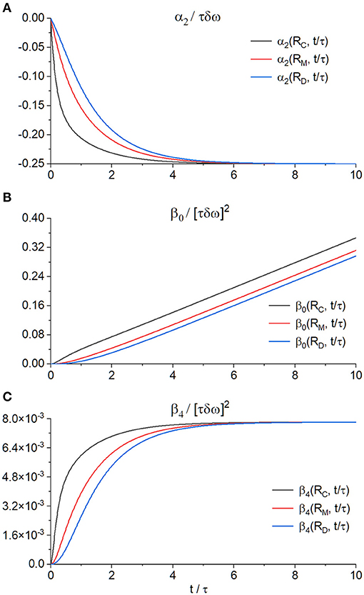
Figure 2. Time evolution of the GLP moment functions α₂(r, t) (A), β₀(r, t) (B), and β₄(r, t) (C) at the discretized radial points R_C, R_M = [R_C + R_D]/2, and R_D for τδω = 10 and η = 0.1.

FIGURE 3

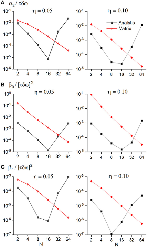
Figure 3. Root mean squared error between the true time evolution of the moment functions α₂(R_C, t) (A), β₀(R_C, t) (B), and β₄(R_C, t) (C) as determined by a finite element simulation of Equations (33)–(35) and either the analytical solution according to Equations (36)–(38) or the finite difference solution according to Equations (73), (78), and (79). The time evolution was calculated from t/τ = 0 to t/τ = 10 in steps of 0.1 either for η = 0.05 (left side) or η = 0.1 (right side). The abscissa represents either the number of considered eigenvalues for the analytic solution or the matrix dimension for the matrix solution.

3.2. Local Magnetization

The discretized local magnetization is in the GLP first order

$\begin{array}{ll}\frac{{\overrightarrow{m}}_I(\varphi ,t)}{m_0}=exp(\text{i}{\alpha }_2(t)cos(2\varphi ))\overrightarrow{1}& (80)\end{array}$

and in the GLP second order

$\begin{array}{ll}\frac{{\overrightarrow{m}}_{II}(\varphi ,t)}{m_0}=exp(\text{i}{\alpha }_2(t)cos(2\varphi )-{\beta }_0(t))\times & (81)\end{array}$

$\begin{array}{ll}exp\left(-{\beta }_4(t)cos(4\varphi )+\frac{1}{2}{\left[{\alpha }_2(t)cos(2\varphi )\right]}^2\right)\overrightarrow{1}.& (82)\end{array}$

These vector equations correspond to the scalar equations (18) and (19). As in the continuous case, the initial magnetization is set to the constant vector $\overrightarrow{1}$ of length N. The time course of the local magnetization reveals a complex relationship between the real and imaginary parts, as shown in Figures 4, 5.

FIGURE 4

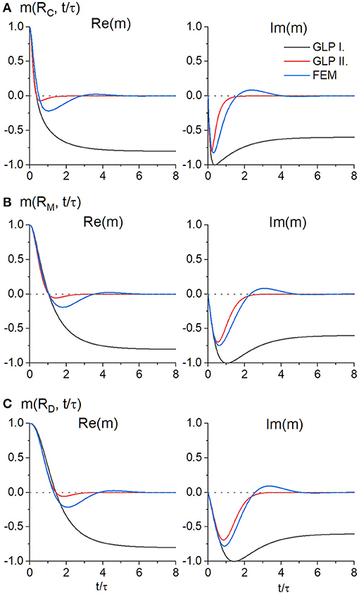
Figure 4. Real and imaginary parts of the local magnetization calculated from the GLP first order according to Equation (80) (black solid line), GLP second order according to Equation (81) (red solid line) or with a finite element simulation of the Bloch-Torrey equation (blue solid line) at the discretized radial points R_C (A), R_M = [R_C + R_D]/2 (B), and R_D (C) for ϕ = 0, τδω = 10 and η = 0.1.

FIGURE 5

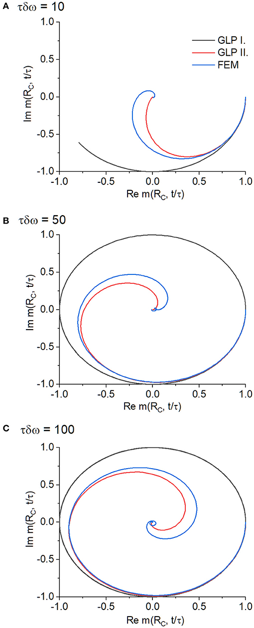
Figure 5. Visualization of the real part and the imaginary part of the local magnetization at R_C and ϕ = 0 for τδω = 10 (A), τδω = 50 (B), and τδω = 100 (C) with η = 0.1. The starting point lies at Re(m(R_C, 0)) = 1, Im(m(R_C, 0)) = 0 for each graph. The oscillatory nature of the local magnetization in the GLP first order can be clearly seen.

3.3. Total Magnetization

For the total magnetization in the discretized case, the Jacobi determinant r in Equation (43) is replaced by the discretized differential area element (see Equation (64) in [26])

$\begin{array}{l}k=\frac{2}{N-1}\frac{\sqrt{\eta }}{1+\sqrt{\eta }}\times \\ \text{diag}\left(\frac{1}{2},1+\frac{1}{N-1}\frac{1-\sqrt{\eta }}{\sqrt{\eta }},\dots ,1+\frac{N-2}{N-1}\frac{1-\sqrt{\eta }}{\sqrt{\eta }},\frac{1}{2\sqrt{\eta }}\right)& (83)\end{array}$

resulting in

$\begin{array}{ll}\frac{M(t)}{M_0}=\frac{1}{2\pi }{\displaystyle \underset{0}{\overset{2\pi }{\int }}}\text{d}\varphi {\overrightarrow{1}}^{⊺}\text{k}\frac{\overrightarrow{m}(\varphi ,t)}{m_0}.& (84)\end{array}$

In the first-order GLP, the angular interval can be solved and the total magnetization can be found by inserting Equation (80) into Equation (84) as

$\begin{array}{ll}\frac{M_I(t)}{M_0}={\overrightarrow{1}}^{⊺}\text{k}{J}_0({\alpha }_2(t))\overrightarrow{1},& (85)\end{array}$

with J₀ being the Bessel function of first kind and zeroth order. In the second-order GLP, the angular integral is not analytically solvable and, therefore, the total magnetization obtained by inserting Equation (81) into Equation (84), remains

$\begin{array}{l}\frac{M_{II}(t)}{M_0}=\frac{1}{2\pi }{\overrightarrow{1}}^{⊺}{\text{k}\text{e}}^{-{\beta }_0(t)}\times \\ {\displaystyle \underset{0}{\overset{2\pi }{\int }}}\text{d}\varphi {\text{e}}^{\text{i}{\alpha }_2(t)cos(2\varphi )-{\beta }_4(t)cos(4\varphi )+\frac{1}{2}{\left[{\alpha }_2(t)cos(2\varphi )\right]}^2}\overrightarrow{1}.& (86)\end{array}$

3.4. Comparison With Other Solutions

In the Gaussian Phase approximation, the total magnetization is equal to

$\begin{array}{ll}\frac{M_{GP}(t)}{M_0}=exp\left(-{\left[\tau \delta \omega \right]}^2{\displaystyle \sum _{n=1}^{\infty }}\frac{F_n^2}{{\lambda }_{n,2}^2}\left[\frac{t}{\tau }+\frac{{\text{e}}^{-{\lambda }_{n,2}^2\frac{t}{\tau }}-1}{{\lambda }_{n,2}^2}\right]\right)& (87)\end{array}$

where the definition of the eigenvalues λ_n,2 is as usual, and the coefficients F_n are defined by

$\begin{array}{ll}{F}_n^2=\frac{\eta }{1-\eta }\frac{{\left[M_{n,2}^{-}\right]}^2}{N_{n,2}},& (88)\end{array}$

with the definitions of N_n,2 given in Equation (14) and the definition of $M_{n,2}^{-}$ given in Equation (B8) in the Appendix. Using Equations (127)–(130) from Ziener et al. [25], this can be further simplified to

$\begin{array}{l}\frac{M_{GP}(t)}{M_0}=\\ exp\left({\left[\tau \delta \omega \right]}^2\left[\frac{\eta \text{ln}(\eta )}{8\left[1-\eta \right]}\frac{t}{\tau }+\frac{1}{32}-{\displaystyle \sum _{n=1}^{\infty }}\frac{F_n^2}{{\lambda }_{n,2}^4}{\text{e}}^{-{\lambda }_{n,2}^2\frac{t}{\tau }}\right]\right).& (89)\end{array}$

The term linearly dependent on the time again has the same form as in Equation (42). Using the discretized version of the correlation function in Equation (A14), the total magnetization in the Gaussian phase approximation can also be written in terms of the Laplace operator:

$\begin{array}{l}\frac{M_{GP}(t)}{M_0}=exp\left(\frac{{\left[\tau \delta \omega \right]}^2}{8}\left[\frac{\eta \text{ln}(\eta )}{1-\eta }\frac{t}{\tau }+\frac{1}{4}\right]\right)\times \\ exp(\frac{{\left[\tau \delta \omega \right]}^2}{64}{\overrightarrow{1}}^{⊺}{\text{kr}}^{-2}{\text{e}}^{\frac{t}{\tau }\left[{\Delta }_r-4{\text{r}}^{-2}\right]}\times \\ \left[{\text{r}}^2\left[2ln(\text{r})-1\right]+\left[{\text{r}}^2+{\text{r}}^{-2}\right]\frac{ln(\eta )}{1-{\eta }^2}\right]\overrightarrow{1}).& (90)\end{array}$

If the magnetization decay is modeled as monoexponential (ME), different approximations for different diffusion strengths exist. If the diffusion term dominates the susceptibility term, called the motional narrowing regime (ME MN), the formula is [27]

$\begin{array}{ll}\frac{M_{\text{ME MN}}(t)}{M_0}=exp\left(-\frac{\eta {\left[\tau \delta \omega \right]}^2}{2}\frac{t}{\tau }\right),& (91)\end{array}$

and in the case of vanishing diffusion, called static dephasing regime (ME SD), it is [27]

$\begin{array}{ll}\frac{M_{\text{ME SD}}(t)}{M_0}=exp\left(-\frac{2\eta \delta \omega }{1+\eta }t\right).& (92)\end{array}$

Both introduced solutions, i.e., the GLP first order and the GLP second order, are compared with the true total magnetization as obtained by a finite element simulation of the Bloch-Torrey equation and other approximations in Figure 6. In order to compare the numerical efficiency of the different approaches, 10 calculation runs of the total magnetization were timed for each method implemented in Mathematica using 24 computation threads in parallel. The results can be seen in Table 1. The matrix calculation methods is several times faster than the analytical calculation method. The finite element simulation is by far the slowest method, in part because of the high spatial and temporal resolution needed to avoid instability in cases of lower diffusion strength.

FIGURE 6

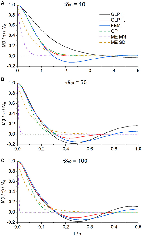
Figure 6. Comparison of the total magnetization for τδω = 10 (A), τδω = 50 (B), and τδω = 100 (C) for η = 0.1. Black solid line: GLP first order according to Equation (85), red solid line: GLP second order according to Equation (86), blue solid line: finite element simulation of the Bloch-Torrey equation (20), green dashed line: Gaussian Phase approximation according to Equation (87), purple dashed line: monoexponential motional narrowing approximation according to Equation (91), and orange dashed line: monoexponential static dephasing approximation according to Equation (92).

TABLE 1

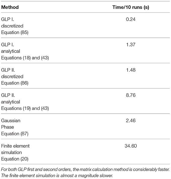
Table 1. Computation time for 10 calculation runs for the total magnetization of the different calculation methods.

4. Discussion and Conclusion

Herein, we derive the GLP approximation for a cylindrical dephasing domain under the influence of the susceptibility effects of a blood-filled inner vessel [6]. We, further, present a solution method based on solving a matrix differential equation which arises from a finite-differences discretization scheme for the Laplace operator. As the phase distribution during magnetic resonance imaging is a complicated time-dependent function of the shape of the dephasing domain, of the diffusion strength and of susceptibility effects, it is often assumed to take a Gaussian form [4, 28, 29]. In the GLP, the ensemble distribution of the local phase is considered instead and the distribution approximated by its first two cumulants. This method of approximating a probability distribution in terms of cumulants rather than moments has been introduced by Kubo [30–32]. Derivations can be found in standard stochastic physics textbooks, e.g., in Chapter XVI section 4 in van Kampen [33] or in Cowan [28]. It has been shown that the GLP approximation leads to a better approximation of the total magnetization in the case of a constant gradient for cylindrical or spherical voxel shapes [5].

As can be seen in Figure 6, out of all options, the GLP approximation of second order has the least deviation from the true total magnetization time evolution. Interestingly, the GLP of first order shows greater deviations from the true total magnetization than the Gaussian Phase approximation. A possible explanation for this may be that in the GLP first order, the local magnetization does not converge to zero as expected, as Figures 4, 5 demonstrate. This leads to undampened oscillatory behavior that ultimately results in a large deviation both for the local and total magnetization. The Gaussian Phase approximation suffers from the opposite behavior: the total magnetization is overdampened and decays monotonically to zero over time. The GLP of second order does not suffer from either of these problems: it is able to follow oscillations to negative total magnetization while having proper dampening. This can also be seen from the definition of the local magnetization in Equation (19). If only the first cumulant is taken into account, the purely real coefficient α(r, t) is multiplied with the imaginary unit i in the exponent and its magnitude can only influence the angular frequency of the oscillations of $m(\overrightarrow{r},t)$. The amplitude of the local magnetization cannot be modulated. This is only possible with the addition of a second cumulant: in this case, both α(r, t) and β(r, t) have non-zero real value in the exponent, which is then able to modulate its amplitude and phase. The local magnetization having constant absolute magnitude does not, however, mean that the total magnetization, corresponding to its domain integral, also has this property: due to destructive (or theoretically constructive) interference, its amplitude can, of course, vary.

From an algorithmic viewpoint, the calculation of the GLP cumulants either requires knowledge of the spectral expansion of the diffusion propagator or, alternatively, a proper finite difference scheme for the Laplacian on the dephasing domain. Both approaches are feasible for bounded domains with rotational symmetry. As Figure 3 demonstrates, the finite-difference approach has the advantage of a monotonically decreasing error in respect to the true solution. The increase in the error for the analytical solution for larger numbers of coefficients is most likely due to the idiosyncrasies of the numerical implementation and may very well not be present if one uses a different implementation of Bessel functions. Both methods, however, are not natively suited for extension to unbounded domains. For the spectral expansion, an increasing number of eigenvalues has to be considered as the dephasing domain becomes larger and larger, until ultimatively the eigenvalue spectrum becomes continuous for a truly unbounded domain. The finite difference scheme can be adapted by either increasing the number of grid points or by adapting the discretization scheme to allow a non-uniform grid with the last point in infinity [34–38]. These problems can most likely be overcome, and may allow extending the GLP approximation method for the cases of dephasing outside of cylinders or spheres [39–42]. Furthermore, the introduced method of comparing expressions for the cumulants for long time ranges allows writing the coefficient equations in a far simpler form. This may also be applicable for cumulant expansions in other models, such as Equations (70) and (82) in Ziener et al. [5].

In our model, we considered dephasing in the domain around a single cylindrical vessel. The influence of neighboring cylinders and possible crossing-over effects was included by imposing reflecting boundary conditions at the outer border. This assumption, however, is true only for an uniform arrangement of capillaries. The signal evolution from randomly arranged capillaries differs significantly. Yablonskiy and Haacke derived the relaxation rates of randomly arranged capillaries or spheres in the absence of diffusion and were able to find an expression for the relaxation rate that is based on a single capillary or sphere, similar to the uniform case [43]. It is unknown, however, if this holds for the non-negligible diffusion effects—numerical simulations of randomly arranged capillaries suggest that this is indeed the case [44], but no proof has been found.

Our model neglects the signal originating from inside the vessel. This is sensible if the volume ratio η is sufficiently low, as the total signal is, of course, the weighted sum of the intra- and extravascular signals. For very short experimental times, the flow inside the vessel can be neglected, and the protons can be assumed to be stationary. The intravascular magnetic field is then homogeneous [12], leading to a complete refocusing of the signal in spin echo experiments. For longer experimental times, the intravascular flow can no longer be neglected. Due to the low laminar flow speeds in the human capillaries, electrodynamic effects are most likely irrelevant, and the intravascular compartment can be modeled separately. To our knowledge, no systematic investigation of such effects has taken place.

The main advantage of GLP approximation and simultaneously its weak point arises from its handling of the interplay of diffusion and susceptibility effects: the diffusion propagator can be calculated separately, usually as the solution of the diffusion equation (or more generally the Fokker-Planck equation in case of a spatially variant diffusion constant [45]) and applied to the susceptibility term at each jump point, once for the first cumulant and twice for the second cumulant [46]. This places very few restrictions on the diffusion propagator, and its calculation does not have to be adapted to the form of the dipole field. Therefore, flow effects and anisotropic diffusion coefficients can be easily considered. Adapting the full Bloch-Torrey equation to such circumstances is rather cumbersome [47].

Data Availability Statement

The original contributions presented in the study are included in the article/Supplementary Material, further inquiries can be directed to the corresponding author/s.

Author Contributions

LR and CZ performed the modeling and wrote the manuscript. CZ provided the initial concept of the article. EW contributed to the mathematical concepts described in the article. EW and H-PS provided the input on organization and presentation of models. All authors contributed to the manuscript revision, read, and approved the submitted version.

Conflict of Interest

The authors declare that the research was conducted in the absence of any commercial or financial relationships that could be construed as a potential conflict of interest.

Supplementary Material

The Supplementary Material for this article can be found online at: https://www.frontiersin.org/articles/10.3389/fphy.2021.662088/full#supplementary-material

References

1. Bloch F. Nuclear induction. Phys Rev. (1946) 70:460–74. doi: 10.1103/PhysRev.70.460

CrossRef Full Text | Google Scholar

2. Torrey HC. Bloch equations with diffusion terms. Phys Rev. (1956) 104:563–5. doi: 10.1103/PhysRev.104.563

CrossRef Full Text | Google Scholar

3. Grebenkov DS. NMR survey of reflected Brownian motion. Rev Mod Phys. (2007) 79:1077–37. doi: 10.1103/RevModPhys.79.1077

CrossRef Full Text | Google Scholar

4. Hahn EL. Spin echoes. Phys Rev. (1950) 80:580–94. doi: 10.1103/PhysRev.80.580

CrossRef Full Text | Google Scholar

5. Ziener CH, Kampf T, Schlemmer HP, Buschle LR. Spin dephasing in the Gaussian local phase approximation. J Chem Phys. (2018) 149:244201. doi: 10.1063/1.5050065

PubMed Abstract | CrossRef Full Text | Google Scholar

6. Krogh A. The number and distribution of capillaries in muscles with calculations of the oxygen pressure head necessary for supplying the tissue. J Physiol. (1919) 52:409–15. doi: 10.1113/jphysiol.1919.sp001839

PubMed Abstract | CrossRef Full Text | Google Scholar

7. Grebenkov DS, Nguyen BT. Geometrical structure of Laplacian Eigenfunctions. SIAM Rev. (2013) 55:601–67. doi: 10.1137/120880173

CrossRef Full Text | Google Scholar

8. Russell G, Harkins KD, Secomb TW, Galons JP, Trouard TP. A finite difference method with periodic boundary conditions for simulations of diffusion-weighted magnetic resonance experiments in tissue. Phys Med Biol. (2012) 57:N35–46. doi: 10.1088/0031-9155/57/4/N35

PubMed Abstract | CrossRef Full Text | Google Scholar

9. Nguyen DV, Li JR, Grebenkov D, Le Bihan D. A finite elements method to solve the Bloch–Torrey equation applied to diffusion magnetic resonance imaging. J Comput Phys. (2014) 263:283–302. doi: 10.1016/j.jcp.2014.01.009

CrossRef Full Text | Google Scholar

10. Beltrachini L, Taylor ZA, Frangi AF. An efficient finite element solution of the generalised Bloch-Torrey equation for arbitrary domains. In: Fuster A, Ghosh A, Kaden E, Rathi Y, Reisert M, editors. Computational Diffusion MRI. Basel: Springer International Publishing (2016). p. 3–14. doi: 10.1007/978-3-319-28588-7_1

PubMed Abstract | CrossRef Full Text | Google Scholar

11. Nguyen VD, Leoni M, Dancheva T, Jansson J, Hoffman J, Wassermann D, et al. Portable simulation framework for diffusion MRI. J Magn Reson. (2019) 309:106611. doi: 10.1016/j.jmr.2019.106611

PubMed Abstract | CrossRef Full Text | Google Scholar

12. Reichenbach JR, Haacke EM. High-resolution BOLD venographic imaging: a window into brain function. NMR Biomed. (2001) 14:453–67. doi: 10.1002/nbm.722

PubMed Abstract | CrossRef Full Text | Google Scholar

13. Ziener CH, Bauer WR, Melkus G, Weber T, Herold V, Jakob PM. Structure-specific magnetic field inhomogeneities and its effect on the correlation time. Magn Reson Imaging. (2006) 24:1341–7. doi: 10.1016/j.mri.2006.08.005

PubMed Abstract | CrossRef Full Text | Google Scholar

14. Robertson B. Spin-echo decay of spins diffusing in a bounded region. Phys Rev. (1966) 151:273–7. doi: 10.1103/PhysRev.151.273

CrossRef Full Text | Google Scholar

15. Stoller SD, Happer W, Dyson FJ. Transverse spin relaxation in inhomogeneous magnetic fields. Phys Rev A. (1991) 44:7459–77. doi: 10.1103/PhysRevA.44.7459

PubMed Abstract | CrossRef Full Text | Google Scholar

16. de Swiet TM, Sen PN. Decay of nuclear magnetization by bounded diffusion in a constant field gradient. J Chem Phys. (1994) 100:5597–604. doi: 10.1063/1.467127

CrossRef Full Text | Google Scholar

17. Moutal N, Demberg K, Grebenkov DS, Kuder TA. Localization regime in diffusion NMR: theory and experiments. J Magn Reson. (2019) 305:162–74. doi: 10.1016/j.jmr.2019.06.016

PubMed Abstract | CrossRef Full Text | Google Scholar

18. Moutal N, Moutal A, Grebenkov D. Diffusion NMR in periodic media: efficient computation and spectral properties. J Phys A Math Theor. (2020) 53:325201. doi: 10.1088/1751-8121/ab977e

CrossRef Full Text | Google Scholar

19. Carslaw HS, Jaeger JC. Conduction of Heat in Solids. 2nd ed. Oxford: Oxford University Press (1986).

Google Scholar

20. Thambynayagam RKM. The Diffusion Handbook: Applied Solutions for Engineers. New York, NY: McGraw-Hill (2011).

21. Ziener CH, Kampf T, Kurz FT. Diffusion propagators for hindered diffusion in open geometries. Concepts Magn Reson A. (2015) 44:150–9. doi: 10.1002/cmr.a.21346

CrossRef Full Text | Google Scholar

22. Glasser ML. Integral representations for the exceptional univariate Lommel functions. J Phys A Math Theor. (2010) 43:155207. doi: 10.1088/1751-8113/43/15/155207

CrossRef Full Text | Google Scholar

23. Bauer WR, Nadler W, Bock M, Schad LR, Wacker C, Hartlep A, et al. Theory of the BOLD effect in the capillary region: an analytical approach for the determination of T2* in the capillary network of myocardium. Magn Reson Med. (1999) 41:51–62. doi: 10.1002/(SICI)1522-2594(199901)41:1<51::AID-MRM9>3.0.CO;2-G

PubMed Abstract | CrossRef Full Text | Google Scholar

24. Ziener CH, Kampf T, Herold V, Jakob PM, Bauer WR, Nadler W. Frequency autocorrelation function of stochastically fluctuating fields caused by specific magnetic field inhomogeneities. J Chem Phys. (2008) 129:014507. doi: 10.1063/1.2949097

PubMed Abstract | CrossRef Full Text | Google Scholar

25. Ziener CH, Kurz FT, Buschle LR, Kampf T. Orthogonality, Lommel integrals and cross product zeros of linear combinations of bessel functions. SpringerPlus. (2015) 4:390. doi: 10.1186/s40064-015-1142-0

PubMed Abstract | CrossRef Full Text | Google Scholar

26. Rotkopf LT, Wehrse E, Kurz FT, Schlemmer HP, Ziener CH. Efficient discretization scheme for semi-analytical solutions of the Bloch-Torrey equation. J Magn Reson Open. (2021) 6–7:100010. doi: 10.1016/j.jmro.2021.100010

CrossRef Full Text | Google Scholar

27. Ziener CH, Kurz FT, Kampf T. Free induction decay caused by a dipole field. Phys Rev E. (2015) 91:032707. doi: 10.1103/PhysRevE.91.032707

PubMed Abstract | CrossRef Full Text | Google Scholar

28. Cowan B. Nuclear Magnetic Resonance and Relaxation. Cambridge: Cambridge University Press (1997). doi: 10.1017/CBO9780511524226

CrossRef Full Text | Google Scholar

29. Callaghan PT. Translational Dynamics and Magnetic Resonance: Principles of Pulsed Gradient Spin Echo NMR. Oxford: Oxford University Press (2011). doi: 10.1093/acprof:oso/9780199556984.001.0001

CrossRef Full Text | Google Scholar

30. Kubo R. Generalized cumulant expansion method. J Phys Soc Jpn. (1962) 17:1100–20. doi: 10.1143/JPSJ.17.1100

CrossRef Full Text | Google Scholar

31. Kubo R. A stochastic theory of line shape. In: Shuler KE, editor. Advances in Chemical Physics. Hoboken, NJ: John Wiley & Sons, Inc. (1969). p. 101–27. doi: 10.1002/9780470143605.ch6

CrossRef Full Text | Google Scholar

32. Nadler W, Schulten K. Generalized moment expansion for Brownian relaxation processes. J Chem Phys. (1985) 82:151–60. doi: 10.1063/1.448788

CrossRef Full Text | Google Scholar

33. van Kampen NG. Stochastic Processes in Physics and Chemistry. 3rd ed. North-Holland Personal Library. Amsterdam: Elsevier (2007). doi: 10.1016/B978-044452965-7/50006-4

CrossRef Full Text | Google Scholar

34. Hagstrom TM, Keller HB. Asymptotic boundary conditions and numerical methods for nonlinear elliptic problems on unbounded domains. Math Comput. (1987) 48:449–9. doi: 10.1090/S0025-5718-1987-0878684-5

CrossRef Full Text | Google Scholar

35. Ehrhardt M. “Finite difference schemes on unbounded domains” In: Mickens RE, editor. Advances in the Applications of Nonstandard Finite Difference Schemes. Vol. 8 of 1. Singapore: World Scientific (2005). p. 343–84. doi: 10.1142/9789812703316_0008

CrossRef Full Text | Google Scholar

36. Fazio R, Jannelli A. BVPs on infinite intervals: a test problem, a nonstandard finite difference scheme and a posteriori error estimator. Math Methods Appl Sci. (2017) 40:6285–94. doi: 10.1002/mma.4456

CrossRef Full Text | Google Scholar

37. Fazio R, Jannelli A, Agreste S. A finite difference method on non-uniform meshes for time-fractional advection–diffusion equations with a source term. Appl Sci. (2018) 8:960. doi: 10.3390/app8060960

CrossRef Full Text | Google Scholar

38. Fazio R, Jannelli A. Finite difference schemes on quasi-uniform grids for BVPs on infinite intervals. J Comput Appl Math. (2014) 269:14–23. doi: 10.1016/j.cam.2014.02.036

CrossRef Full Text | Google Scholar

39. Kurz FT, Kampf T, Heiland S, Bendszus M, Schlemmer HP, Ziener CH. Theoretical model of the single spin-echo relaxation time for spherical magnetic perturbers. Magn Reson Med. (2014) 71:1888–95. doi: 10.1002/mrm.25196

PubMed Abstract | CrossRef Full Text | Google Scholar

40. Yung KT. Empirical models of transverse relaxation for spherical magnetic perturbers. Magn Reson Imaging. (2003) 21:451–63. doi: 10.1016/S0730-725X(02)00640-9

PubMed Abstract | CrossRef Full Text | Google Scholar

41. Kraiger M, Schnizer B. Potential and field of a homogeneous magnetic spheroid of arbitrary direction in a homogeneous magnetic field in Cartesian coordinates. COMPEL. (2013) 32:936–60. doi: 10.1108/03321641311305845

CrossRef Full Text | Google Scholar

42. Jensen JH, Chandra R. NMR relaxation in tissues with weak magnetic inhomogeneities. Magn Reson Med. (2000) 44:144–56. doi: 10.1002/1522-2594(200007)44:1<144::AID-MRM21>3.0.CO;2-O

PubMed Abstract | CrossRef Full Text | Google Scholar

43. Yablonskiy DA, Haacke EM. Theory of NMR signal behavior in magnetically inhomogeneous tissues: the static dephasing regime. Magn Reson Med. (1994) 32:749–63. doi: 10.1002/mrm.1910320610

PubMed Abstract | CrossRef Full Text | Google Scholar

44. Buschle LR, Kurz FT, Kampf T, Schlemmer HP, Ziener CH. Spin dephasing around randomly distributed vessels. J Magn Reson. (2019) 299:12–20. doi: 10.1016/j.jmr.2018.11.014

PubMed Abstract | CrossRef Full Text | Google Scholar

45. Tanimura Y. Stochastic Liouville, Langevin, Fokker–Planck, and master equation approaches to quantum dissipative systems. J Phys Soc Jpn. (2006) 75:39. doi: 10.1143/JPSJ.75.082001

CrossRef Full Text | Google Scholar

46. Stepisnik J. A new view of the spin echo diffusive diffraction in porous structures. Europhys Lett. (2002) 60:453–9. doi: 10.1209/epl/i2002-00285-3

CrossRef Full Text

47. Seroussi I, Grebenkov DS, Pasternak O, Sochen N. Microscopic interpretation and generalization of the Bloch-Torrey equation for diffusion magnetic resonance. J Magn Reson. (2017) 277:95–103. doi: 10.1016/j.jmr.2017.01.018

PubMed Abstract | CrossRef Full Text | Google Scholar