Semiflexible Polymer Enclosed in a 3D Compact Domain

The conformational states of a semiflexible polymer enclosed in a volume $V:={\ell }^3$ are studied as stochastic realizations of paths using the stochastic curvature approach developed in [Rev. E 100, 012503 (2019)], in the regime whenever $3\ell /{\ell }_p>1$, where ${\ell }_p$ is the persistence length. The cases of a semiflexible polymer enclosed in a cube and sphere are considered. In these cases, we explore the Spakowitz–Wang–type polymer shape transition, where the critical persistence length distinguishes between an oscillating and a monotonic phase at the level of the mean-square end-to-end distance. This shape transition provides evidence of a universal signature of the behavior of a semiflexible polymer confined in a compact domain.

1 Introduction

Semiflexible polymers is a term coined to understand a variety of physical systems that involve linear molecules. The most popular polymers are industrial plastics, like polyethylene or polystyrene, with various applications in daily life [1, 2]. Another prominent example is the DNA compacted in the nucleus of cells or viral DNA/RNA packed in capsids [3, 4]. These last examples are of particular interest since they are confined semiflexible polymers. Indeed, biopolymers’ functionality is ruled by their conformation, which in turn is considerably modified in the geometrically confined or crowded environment inside the cell [5–7].

A common well-known theoretical framework used to describe the fundamental properties of a semiflexible polymer is the well-known worm-like chain model (WLC), which pictures a polymer as a thin wire with a flexibility given by its bending rigidity constant α [8]. The central quantity in this model is the persistence length defined by $2\alpha /\left(k_{B}T\left(d-1\right)\right)$ [9, 10], with d being the space dimension; however, here we simply use ${\ell }_p:=\alpha /\left(k_{B}T\right)$¹, which is the characteristic length along the chain over which the directional correlation between segments disappears. $k_{B}T$ is the thermal energy, with $k_B$ and T being the Boltzmann constant and the bath temperature, respectively [11].

In the absence of thermal fluctuations, when $\alpha \gg k_{B}T$, the conformations of the polymer are well understood through different curve configurations determined by variational principles [12, 13]. For the WLC model, the bending energy functional is given by

$H\left[\mathbf{R}\right]=\frac{\alpha }{2}{\displaystyle \int ds{\kappa }^2\left(s\right)},(1)$

where $\mathbf{R}\left(s\right)$ is a polymer configuration and $\kappa \left(s\right)$ is the curvature of the chain, with s being the arc-length parameter. Additional terms can be added to the Hamiltonian to account for other effects, including multibody interactions, external fields, and constraints on the chain dimensions [14, 15]. When the thermal fluctuations are relevant, that is, $\alpha \simeq k_{B}T$, then it is usual to introduce a statistical mechanics description. Since $H\left[\mathbf{R}\right]$ represents the bending energy for a curve configuration $\mathbf{R}$, the most natural approach is to define the canonical probability density

$\mathcal{P}\left(\mathit{R}\right)\mathcal{D}\mathit{R}:=\frac{1}{{\mathcal{Z}}_{\text{c}}}\text{exp}\left(-\frac{{\ell }_p}{2}{\displaystyle \int ds{\kappa }^2\left(s\right)}\right)\mathcal{D}\mathit{R}\text{,}(2)$

where ${\mathcal{Z}}_{\text{c}}$ is the canonical partition function and $\mathcal{D}\mathit{R}$ is an appropriate functional measure. In this description, the theory turns out to be a one-dimensional statistical field theory. Nonetheless, the theory is not easy to tackle since $\kappa \left(s\right)$ acquires nonlinear terms in $\mathbf{R}$. To avoid this difficulty, a different perspective was introduced by Saito’s et al. [8], where the following probability density function was studied:

$\mathcal{P}\left(\mathit{T}\right)\mathcal{D}\mathit{T}:=\frac{1}{{\mathcal{Z}}_{\text{s}}}\exp \left(-\frac{{\ell }_p}{2}{\displaystyle \int ds{\kappa }^2\left(s\right)}\right)\mathcal{D}\mathit{T}\text{,}(3)$

instead of Eq. 2. Here ${\mathcal{Z}}_{\text{s}}$ is the Saito’s partition function and $\mathcal{D}\mathbf{T}$ is an appropriate functional measure for the tangent direction of a given polymer configuration $\mathbf{R}$. The Saito’s partition function can be solved since one has ${\kappa }^2\left(s\right)={\left(d\mathbf{T}\left(s\right)/ds\right)}^2$; thus, one can relate ${\mathcal{Z}}_{\text{s}}$ with the Feynman’s partition function for a quantum particle in the spherical surface described by ${\mathbf{T}}^2=1$. For the cases when the semiflexible polymer is in an open Euclidean space, the Saito’s approach works very well. For instance, it reproduces the standard results of Kratky–Porod [16], among other results [8, 14]. However, for the cases when the semiflexible polymer is confined to a bounded region of the space, the Saito’s approach is difficult to use, with some exceptional cases like the situation for semiflexible polymers confined to a spherical shell [24].

For semiflexible polymers in plane space, an alternative theoretical approach to the above formalisms was introduced in [17]. This consists of postulating that each conformational realization of any polymer in the plane is described by a stochastic path satisfying the stochastic Frenet equations, defined by $\frac{d}{ds}\mathbf{R}\left(s\right)=\mathbf{T}\left(s\right)$ and $\frac{d}{ds}\mathbf{T}\left(s\right)=\kappa \left(s\right)\mathbf{N}\left(s\right)$, where $\mathbf{R}\left(s\right)$ is the configuration of the polymer, $\mathbf{T}\left(s\right)$ is the tangent vector to the curve describing the chain at s, $\mathbf{N}\left(s\right):=\mathbf{\in }\mathbf{T}\left(s\right)$ is the normal stochastic unit vector, with $\mathbf{\in }$a rotation by an angle of $\pi /2$, and $\kappa \left(s\right)$ is the stochastic curvature that satisfies the following probability density function:

$\mathcal{P}\left(\kappa \right)\mathcal{D}\kappa :=\frac{1}{{\mathcal{Z}}_{\text{s}-\text{c}}}\exp \left(-\frac{{\ell }_p}{2}{\displaystyle \int ds{\kappa }^2\left(s\right)}\right)\mathcal{D}\kappa ,(4)$

where ${\mathcal{Z}}_{\text{s}-\text{c}}$ is the partition function in the stochastic curvature formalism and $\mathcal{D}\kappa$ is an appropriate measure for the curvature. This, in particular, implies a white noise-like structure, that is, $\langle \kappa \left(s\right)\rangle =0$ and $\langle \kappa \left(s\right)\kappa \left(s^{\prime }\right)\rangle =\delta \left(s-s^{\prime }\right)/{\ell }_p$ [17]. This theoretical framework successfully explains, by first principles, the Kratky–Porod results for free chains confined to an open 2D-plane. Moreover, it correctly describes the mean-square end-to-end distance for semiflexible polymers confined to a square box, a key descriptor of the statistical behavior of a polymer chain.

In the present work, we carry out an extension of the stochastic curvature approach for semiflexible polymers in the three-dimensional space ${\mathrm{ℝ}}^3$. In particular, we analyze the conformational states of a semiflexible polymer enclosed in a bounded region in three-dimensional space. This polymer is in a thermal bath with a uniform temperature. The shapes adopted by the polymer are studied through the mean-square end-to-end distance as a function of the polymer total length as well as its persistence length. In particular, we analyze the cases of a polymer confined to a cube of side a and a sphere of radius R.

The plan of this article is as follows. In Section 2, we introduce the stochastic Frenet equations for the semiflexible polymers in three-dimensional spaces, and by using a standard procedure, we derive the corresponding Fokker–Planck equation. In particular, the Kratky–Porod result for polymers in a 3D open space is obtained. Section 3 contains the derivation of the mean-square end-to-end distance for semiflexible polymers confined to a compact domain. In Section 4, we present the analysis of the mean square end-to-end distance for the cases when the compact domain corresponds with a cube of side a and a sphere of radius R. Finally, Section 5 contains our concluding remarks.

2 Preliminary Notation and Semiflexible Polymers in 3D

Let us consider a polymer in a three-dimensional Euclidean space ${\mathrm{ℝ}}^3$ as a space curve γ, $\mathbf{R}:I\subset \mathrm{ℝ}\to {\mathrm{ℝ}}^3$, parametrized by an arc-length, s. For each point $s\in I$, a Frenet–Serret trihedron can be defined in terms of the vector basis $\left\{\mathbf{T}\left(s\right),\mathbf{N}\left(s\right),\mathbf{B}\left(s\right)\right\}$, where $\mathbf{T}\left(s\right)=d\mathbf{R}/ds$ is the tangent vector, whereas $\mathbf{N}\left(s\right)$ and $\mathbf{B}\left(s\right)$ are the normal and bi-normal vectors, respectively. It is well known that each regular curve γ satisfies the Frenet–Serret structure equations, namely, $d\mathbf{T}/ds=\kappa \left(s\right)\mathbf{N}$, $d\mathbf{N}/ds=-\kappa \left(s\right)\mathbf{T}-\tau \left(s\right)\mathbf{B}$ and $d\mathbf{B}/ds=\tau \left(s\right)\mathbf{N}$, where $\kappa \left(s\right)$ and $\tau \left(s\right)$ are the curvature and the torsion of the space curve, respectively. In addition, the fundamental theorem of space curves estates that given continuous functions $\kappa \left(s\right)$ and $\tau \left(s\right)$, one can determine the shape curve uniquely, up to a Euclidean rigid motion [18].

2.1 Stochastic Curvature Approach in 3D

In order to study the conformational states of a semiflexible polymer, we adapt the stochastic curvature approach introduced in [17] to the case of semiflexible polymers in 3D Euclidean space. For the 2D Euclidean space, the formalism starts by postulating that each conformational realization of any polymer is described by a stochastic path satisfying the stochastic Frenet equations. In the 3D case, it is enough to consider the following stochastic equations:

$\frac{d}{ds}\mathbf{R}\left(s\right)=\mathbf{T}\left(s\right),(\mathrm{5a})$

$\frac{d}{ds}\mathbf{T}\left(s\right)={\mathrm{\mathbb{P}}}_{\mathbf{T}}\mathit{\kappa }\left(s\right),(\mathrm{5b})$

where $\mathbf{R}\left(s\right)$, $\mathbf{T}\left(s\right)$, and $\mathit{\kappa }\left(s\right)$ are now random variables. Here, $\mathit{\kappa }\left(s\right)$ is named as stochastic vectorial curvature. Also, a normal projection operator ${\mathrm{\mathbb{P}}}_{\mathbf{T}}=1-\mathbf{T}\otimes \mathbf{T}$ has been introduced such that $\mathbf{T}\left(s\right)\cdot \frac{d}{ds}\mathbf{T}\left(s\right)=0$. According to these equations, it can be shown that $\left|\mathbf{T}\left(s\right)\right|$ is a constant that can be fixed to unit, where $\left|\right|$ is the standard 3D Euclidean norm. The remaining geometrical notions also turn into random variables as follows. The stochastic curvature is defined by $\kappa \left(s\right):=\left|\mathit{\kappa }\left(s\right)\right|$. The stochastic normal and bi-normal vectors are defined by $\mathbf{N}\left(s\right):=\mathit{\kappa }\left(s\right)/\kappa \left(s\right)$ and $\mathbf{B}\left(s\right):=\mathbf{T}\left(s\right)\times \mathit{\kappa }\left(s\right)/\kappa \left(s\right)$, respectively, where $\kappa \left(s\right)$ is the stochastic curvature. In addition, the stochastic torsion is defined with the equation $\tau \left(s\right):=\mathbf{N}\left(s\right)\cdot \frac{d}{ds}\mathbf{B}\left(s\right)$.

In addition to the stochastic Eq. 5a and Eq. 5b, the random variable $\mathit{\kappa }\left(s\right)$ is distributed according to the probability density function

$\mathcal{P}\left(\mathit{\kappa }\right)\mathcal{D}\mathit{\kappa }:=\frac{1}{{\mathcal{Z}}_{\text{s}-\text{c}}}\text{exp}\left(-\beta H\left[\mathit{\kappa }\right]\right)\mathcal{D}\mathit{\kappa }\text{,}(6)$

where $H\left[\mathit{\kappa }\right]=\frac{\alpha }{2}{\displaystyle \int {\mathit{\kappa }}^{2}ds}$ is the bending energy and α is the bending rigidity modulus. This energy functional corresponds to the continuous form of the WLC model [8]. Also, in Eq. 6, ${\mathcal{Z}}_{\text{s}-\text{c}}$ is an appropriate normalization constant, $\mathcal{D}\mathit{\kappa }:={\displaystyle {\prod }_{i=1}^3\mathcal{D}{\kappa }_i}$ is a functional measure, and $\beta =1/k_{B}T$ is the inverse of the thermal energy. The Gaussian structure of the probability density implies the zero mean $\langle {\kappa }_i\left(s\right)\rangle =0$ and the following $3D$ fluctuation theorem:

$\langle {\kappa }_i\left(s\right){\kappa }_j\left(s^{\prime }\right)\rangle =\frac{1}{{\ell }_p}{\delta }_{ij}\delta \left(s-s^{\prime }\right),(7)$

where ${\kappa }_i\left(s\right)$ is the $i-$th component of the stochastic vectorial curvature $\mathit{\kappa }\left(s\right)$.

2.2 From Frenet–Serret Stochastic Equations to Hermans–Ullman Equation in 3D

In this section, we present the Fokker–Planck formalism corresponding to the stochastic Eq. 5a and Eq. 5b. This description allows us to determine an equation for the probability density function associated to the position and direction of the endings of the polymer $P\left(\mathbf{R},\mathbf{T}|{\mathbf{R}}^{\prime },{\mathbf{T}}^{\prime };s\right)=\langle \delta \left(\mathbf{R}-\mathbf{R}\left(s\right)\right)\delta \left(\mathbf{T}-\mathbf{T}\left(s\right)\right)\rangle$, where $\mathbf{R}$ and ${\mathbf{R}}^{\prime }$ are the ending positions of the polymer, and $\mathbf{T}$ and ${\mathbf{T}}^{\prime }$ are the corresponding directions, respectively. The parameter s is the polymer length.

Now, the stochastic Frenet–Serret Eq. 5a and Eq. 5b can be identified with a multidimensional stochastic differential equation in the Stratonovich perspective; thus, applying the standard procedure [19], we find the following Fokker–Planck type equation:

$\frac{\partial P}{\partial s}+\nabla \cdot \left(\mathbf{T}P\right)=\frac{1}{2{\ell }_p}{\text{Δ}}_{g}P,(8)$

where $\mathbf{T}$ is identified with the unit normal vector on $S^2$, thus satisfying the condition ${\mathbf{T}}^2=1$. The operator ${\text{Δ}}_g$ is the Laplace–Beltrami of the sphere $S^2$. Similarly, as the situation for semiflexible polymers confine to a plane space [17], this equation is exactly the same as the one obtained by Hermans and Ullman in 1952 [20], where the heuristic parameter they included can now be identified exactly with $1/\left(2{\ell }_p\right)$. In addition, we can make a contact with the Saito’s approach [8] by considering the marginal probability density function:

${\mathcal{Z}}_{\text{s}}\left(\mathbf{T},{\mathbf{T}}^{\prime },s\right)\propto {\displaystyle \int d^3\mathbf{R}{d}^3{\mathbf{R}}^{\prime }P\left(\mathbf{R},\mathbf{T}|{\mathbf{R}}^{\prime },{\mathbf{T}}^{\prime },s\right)}.(9)$

Using the Hermans–Ullman equation, we can show that ${\mathcal{Z}}_{\text{c}}$ satisfies a diffusion equation on a spherical surface with diffusion coefficient equal to $1/\left(2{\ell }_p\right)$ [8], that is,

$\frac{\partial {\mathcal{Z}}_{\text{c}}}{\partial s}=\frac{1}{2{\ell }_p}{\text{Δ}}_{S^2}{\mathcal{Z}}_{\text{s}}.(10)$

An immediate consequence of the above equation is the exponential decay of the correlation function between the two ending directions $C\left(L\right):=\langle \mathbf{T}\left(L\right)\cdot \mathbf{T}\left(0\right)\rangle =\text{exp}\left(-L/{\ell }_p\right)$, where L is the polymer length. Indeed, this expectation value satisfies the following equation: $\frac{d}{ds}C\left(s\right)=\frac{1}{2{\ell }_p}\frac{1}{4\pi }{\displaystyle {\int }_{S^2}d\text{Ω}\left(\mathbf{T}\left(s\right)\cdot \mathbf{T}\left(s^{\prime }\right)\right){\text{Δ}}_{S^2}\mathrm{\mathbb{Z}}}$, where $d\text{Ω}$ is the solid angle and $4\pi$ is a normalization constant. Now, we can integrate twice by parts the r.h.s of last equation and since $S^2$ is a compact manifold the boundary terms vanish. Also, using ${\text{Δ}}_{S^2}\mathbf{T}=-\frac{2}{R^2}\mathbf{T}$, it is found that the correlation function satisfies the ordinary differential equation $\frac{d}{ds}C\left(s\right)=-\frac{2}{R^2}C\left(s\right)$. Now, we solve this equation using the initial condition $C\left(s^{\prime }=0\right)=1$ and the length of the polymer set up by $s=L$.

2.3 Modified Telegrapher Equation

As in the situation of the two-dimensional case [17], we carry out a multipolar decomposition for HU equation in 3D. This consists of expanding the probability density function $P\left(\mathbf{R},\mathbf{T}|{\mathbf{R}}^{\prime },{\mathbf{T}}^{\prime };s\right)$ in a linear combination of the Cartesian tensor basis elements 1, $T_i$, $T_i{T}_j-\frac{1}{3}{\delta }_{ij}$, $T_i{T}_j{T}_k-\frac{1}{5}{\delta }_{(ij}{T}_{k)}$, $\cdots$, where the symbols $\left(ijk\right)$ means symmetrization of the indices $i,j,\text{ and }k$, that is, ${\delta }_{(ij}{T}_{k)}={\delta }_{ij}{T}_k+{\delta }_{jk}{T}_i+{\delta }_{ki}{T}_j$ whose expansion coefficients are hydrodynamic-like tensor fields. These tensors are $\rho \left(\mathbf{R},s\right)$, meaning by the manner how the ending positions are distributed in the space; $\mathrm{\mathbb{P}}\left(\mathbf{R},s\right)$, meaning as the local average of the polymer direction; ${\mathrm{\mathbb{Q}}}_{ij}\left(\mathbf{R},s\right)$, pointing the way how the directions are correlated along the points of the space, etc. These tensors are the moments associated to the Cartesian tensor basis, for example, ${\mathrm{\mathbb{P}}}_i={{\displaystyle \int }}^{\text{}}\frac{d\text{Ω}}{4\pi }{T}_{i}P\left(\mathbf{R},\mathbf{T},s\right)$. These fields satisfy the following hierarchy equations:

$\frac{\partial \rho \left(\mathbf{R},s\right)}{\partial s}=-{\partial }_i{\mathrm{\mathbb{P}}}^i\left(\mathbf{R},s\right),(11)$

$\frac{\partial {\mathrm{\mathbb{P}}}_i\left(\mathbf{R},s\right)}{\partial s}=-\frac{1}{{\ell }_p}{\mathrm{\mathbb{P}}}_i\left(\mathbf{R},s\right)-\frac{1}{3}{\partial }_i\rho \left(\mathbf{R},s\right)-{\partial }^j{\mathrm{\mathbb{Q}}}_{ij}\left(\mathbf{R},s\right),(12)$

$\frac{\partial {\mathrm{\mathbb{Q}}}_{ij}\left(\mathbf{R},s\right)}{\partial s}=-\frac{3}{{\ell }_p}{\mathrm{\mathbb{Q}}}_{ij}\left(\mathbf{R},s\right)-\frac{1}{5}{\mathbb{T}}_{ij}\left(\mathbf{R},s\right)-{\partial }^k{\mathrm{ℝ}}_{ijk}\left(\mathbf{R},s\right),(13)$

where ${\mathbb{T}}^{ij}={\partial }^i{\mathrm{\mathbb{P}}}^j+{\partial }^j{\mathrm{\mathbb{P}}}^i-\frac{2{\delta }^{ij}}{3}{\partial }_k{\mathrm{\mathbb{P}}}^k$.

Now, by combining Eq. 11 and Eq. 12, we can obtain a modified telegrapher equation:

$\frac{{\partial }^2\rho \left(\mathbf{R},s\right)}{\partial s^2}+\frac{1}{{\ell }_p}\frac{\partial \rho \left(\mathbf{R},s\right)}{\partial s}=\frac{1}{3}{\nabla }^2\rho \left(\mathbf{R},s\right)+{\partial }_i{\partial }_j{\mathrm{\mathbb{Q}}}^{ij}\left(\mathbf{R},s\right),(14)$

where ${\nabla }^2$ is the 3D Laplacian. In a mean-field point of view, one can consider the preceding equation as an equation for the probability density function $\rho \left(\mathbf{R},s\right)$ under the presence of a mean-field ${\mathrm{\mathbb{Q}}}_{ij}\left(\mathbf{R},s\right)$. In particular, ${\mathrm{\mathbb{Q}}}_{ij}\left(\mathbf{R},s\right)$ does not play any role for the mean-square end-to-end distance for a semiflexible polymer in the open Euclidean 3D space. Indeed, let us define the end-to-end distance as $\delta \mathbf{R}:=\mathbf{R}-{\mathbf{R}}^{\prime }$; thus, the mean-square end-to-end distance is given by

${\langle \delta {\mathbf{R}}^2\rangle }_{\mathcal{D}}\equiv {\displaystyle {\int }_{\mathcal{D}\times \mathcal{D}}\rho \left(\mathbf{R}|{\mathbf{R}}^{\prime },s\right)\delta {\mathbf{R}}^2{d}^3\mathbf{R}{d}^3{\mathbf{R}}^{\prime }}.(15)$

Now, we implement the same procedure used in [17] to calculate the mean-square end-to-end distance in the open three-dimensional space $\mathcal{D}={\mathrm{ℝ}}^3$, where it is used as the modify telegrapher of Eq. 14 and the traceless property of ${\mathrm{\mathbb{Q}}}_{ij}\left(\mathbf{R},s\right)$. We can reproduce the standard Kratky–Porod [16] result for a semiflexible polymer in the three-dimensional space [16, 20].

${\langle \delta {\mathbf{R}}^2\rangle }_{{\mathrm{ℝ}}^3}=2{\ell }_{p}L-2{\ell }_p^2\left(1-\text{exp}\left(-\frac{L}{{\ell }_p}\right)\right)(16)$

with the typical well-known asymptotic limits: diffusive regime $\langle \delta {\mathbf{R}}^2\rangle \simeq 2{\ell }_{p}L$ for $L\gg {\ell }_p$, and ballistic regime $\langle \delta {\mathbf{R}}^2\rangle \simeq L^2$ for $L\ll {\ell }_p$.

3 Semiflexible Polymer in a Compact Domain

In this section, we apply the hierarchy equations developed in the previous section in order to determine the conformational states of a semiflexible polymer confined to a compact volume domain of size V. From the hierarchy Eq. 12 and Eq. 13, the tensors ${\mathrm{\mathbb{P}}}_i\left(\mathbf{R},s\right)$ and ${\mathrm{\mathbb{Q}}}_{ij}\left(\mathbf{R},s\right)$ damp out as $e^{-L/{\ell }_p}$ and $e^{-3L/{\ell }_p}$, respectively. Furthermore, if we consider that the semiflexible polymer is enclosed in a compact volume $V:={\ell }^3$, with a typical length $\ell$; thus, as long as we consider cases when $3\ell /{\ell }_p$ is far from one, we may assume that ${\mathrm{\mathbb{Q}}}_{ij}\left(\mathbf{R},s\right)$ is uniformly distributed. This condition corresponds to truncate the hierarchy equations at the second level; that is, the only equations that survive in this approximation are Eq. 11 and Eq. 12.

In the latter situation, the distribution $\rho \left(\mathbf{R},s\right)$ of the endings of the semiflexible polymer is described through the following telegrapher’s equation:

$\frac{{\partial }^2\rho \left(\mathbf{R},s\right)}{\partial s^2}+\frac{1}{{\ell }_p}\frac{\partial \rho \left(\mathbf{R},s\right)}{\partial s}=\frac{1}{3}{\nabla }^2\rho \left(\mathbf{R},s\right)(17)$

that satisfies the initial conditions

$\underset{s\to 0}{\text{lim}}\rho \left(\mathbf{R}|{\mathbf{R}}^{\prime },s\right)={\delta }^{\left(3\right)}\left(\mathbf{R}-{\mathbf{R}}^{\prime }\right),(18)$

$\underset{s\to 0}{\text{lim}}\frac{\partial \rho \left(\mathbf{R}|{\mathbf{R}}^{\prime },s\right)}{\partial s}=0.(19)$

The condition Eq. 18 means that the polymers’ ends coincide when the polymer length is zero, whereas Eq. 19 means that the polymer length does not change spontaneously. In addition, since the polymer is enclosed in the compact domain $\mathcal{D}$ of volume $V\left(\mathcal{D}\right)$, we also impose a Neumann boundary condition

$\nabla \rho \left(\mathbf{R}|{\mathbf{R}}^{\prime },s\right){|}_{\mathbf{R},{\mathbf{R}}^{\prime }\in \partial D}=0,\forall s,(20)$

where $\partial D$ is a surface bounding the domain $\mathcal{D}$. This boundary condition means that the polymer does not cross the boundary neither wrap the domain. The procedure to obtain a solution of the above telegrapher’s Eq. 17 is identical to the one developed in [17]. We just have to take into account the right factors and the dimensionality considerations. In this sense, the probability density function is given by

$\rho \left(\mathbf{R}|{\mathbf{R}}^{\prime };s\right)=\frac{1}{V\left(\mathcal{D}\right)}{\displaystyle \sum }_{\mathbf{k}\in I}G\left(\frac{s}{2{\ell }_p},\frac{4{\ell }_p^2}{3}{\lambda }_{\mathbf{k}}\right){\psi }_{\mathbf{k}}^{†}\left(\mathbf{R}\right){\psi }_{\mathbf{k}}\left({\mathbf{R}}^{\prime }\right),(21)$

where we recall from [17].

$G\left(v,w\right)=e^{-v}\left[\text{cosh}\left(v\sqrt{1-w}\right)+\frac{\text{sinh}\left(v\sqrt{1-w}\right)}{\sqrt{1-w}}\right](22)$

and $\left\{{\psi }_{\mathbf{k}}\right\}$ and $\left\{{\lambda }_{\mathbf{k}}\right\}$ are a complete set of orthonormal eigenfunctions and a set of corresponding eigenvalues of the Laplace operator $-{\nabla }^2$ in ${\mathrm{ℝ}}^3$. Notice that each ${\psi }_{\mathbf{k}}\left(\mathbf{R}\right)$ must satisfy the Neumann boundary equation $\nabla {\psi }_{\mathbf{k}}{|}_{\mathbf{R}\in \partial \mathcal{D}}=0$. In addition, it is known [21, 22] that for Neumann boundary Laplacian eigenvalue problem, there is a zero eigenvalue ${\lambda }_0=0$ corresponding to a positive eigenfunction given by ${\psi }_0=1/\sqrt{V}$.

Now, using Eq. 21, the mean-square end-to-end distance ${\langle \delta {\mathbf{R}}^2\rangle }_{\mathcal{D}}$ can be computed in the standard fashion by

${\langle {\left(\delta \mathbf{R}\right)}^2\rangle }_{\mathcal{D}}={\displaystyle \sum }_{\mathbf{k}\in I}{a}_{k}G\left(\frac{s}{2{\ell }_p},\frac{4{\ell }_p^2}{3}{\lambda }_{\mathbf{k}}\right),(23)$

where the coefficients of $a_k$ are obtained from

$a_k=\frac{1}{V\left(\mathcal{D}\right)}{\displaystyle {\int }_{\mathcal{D}\times \mathcal{D}}{\left(\mathbf{R}-{\mathbf{R}}^{\prime }\right)}^2{\psi }_{\mathbf{k}}^{†}\left(\mathbf{R}\right){\psi }_{\mathbf{k}}\left({\mathbf{R}}^{\prime }\right)d^3\mathbf{R}{d}^3{\mathbf{R}}^{\prime }}.(24)$

We can have a further simplification after squaring the end-to-end distance inside the last integral. It is not difficult to see that the square terms ${\mathbf{R}}^2$ and ${{\mathbf{R}}^{\prime }}^2$ in ${\left(\mathbf{R}-{\mathbf{R}}^{\prime }\right)}^2$ only the zero mode contribute; thus, we have

${\langle {\left(\delta \mathbf{R}\right)}^2\rangle }_{\mathcal{D}}=2{\sigma }^2\left(\mathbf{R}\right)-\frac{2}{V\left(\mathcal{D}\right)}{\displaystyle \sum }_{\mathbf{k}\ne 0}{\mathbf{r}}_{\mathbf{k}}^{\text{*}}\cdot {\mathbf{r}}_{\mathbf{k}}G\left(\frac{s}{2{\ell }_p},\frac{4{\ell }_p^2}{3}{\lambda }_{\mathbf{k}}\right),(25)$

where ${\sigma }^2\left(\mathbf{R}\right):={\langle {\mathbf{R}}^2\rangle }_g-{\langle \mathbf{R}\rangle }_g^2$ is called the mean-square end position, ${\langle \cdots \rangle }_g:=\frac{1}{V\left(\mathcal{D}\right)}{\displaystyle {\int }_{\mathcal{D}}{d}^3\mathbf{R}\cdots }$ is termed as the geometric average, and the factor ${\mathbf{r}}_{\mathbf{k}}:=\underset{\mathcal{D}}{{\displaystyle \int }}\mathbf{R}{\psi }_{\mathbf{k}}\left(\mathbf{R}\right)d^3\mathbf{R}$ for $\mathbf{k}\ne 0$. The factor ${\mathbf{r}}_{\mathbf{k}}$ can be written in a simpler form for Neumann boundary conditions, since ${\psi }_{\mathbf{k}}=-\frac{1}{{\lambda }_{\mathbf{k}}}{\nabla }^2{\psi }_{\mathbf{k}}$, and by integrating out by parts, this factor is expressed in terms of a boundary integral

${\mathbf{r}}_{\mathbf{k}}=\frac{1}{{\lambda }_{\mathbf{k}}}{\displaystyle {\oint }_{\partial \mathcal{D}}dS\mathbf{n}{\psi }_{\mathbf{k}}\left({\mathbf{R}}_S\right)},(26)$

where ${\mathbf{R}}_S\in \partial \mathcal{D}$ and $dS$ is the area element of $\partial \mathcal{D}$. Since the function $G\left(v,w\right)$ decays exponentially as the polymer length gets larger values, we can convince ourselves that twice the mean-square end position corresponds to a saturation value for the mean-square end-to-end distance. An additional property of ${\mathbf{r}}_{\mathbf{k}}$ is the identity

$\frac{1}{V\left(\mathcal{D}\right)}{\displaystyle \sum }_{\mathbf{k}\ne 0}{\mathbf{r}}_k^{\text{*}}{\mathbf{r}}_{\mathbf{k}}={\sigma }^2\left(\mathbf{R}\right).(27)$

This identity can be proved using the completeness relation of the eigenfunctions, that is, ${\displaystyle \sum }_{\mathbf{k}}{\psi }_{\mathbf{k}}^{\text{*}}\left(\mathbf{R}\right){\psi }_{\mathbf{k}}\left({\mathbf{R}}^{\prime }\right)={\delta }^{\left(3\right)}\left({\mathbf{R}}^{\prime }-\mathbf{R}\right)$. This identity allows us to prove that in general ${\langle {\left(\delta \mathbf{R}\right)}^2\rangle }_{\mathcal{D}}$ starts at zero.

4 Results

4.1 Semiflexible Polymer Enclosed by a Cube Surface

In this section, we provide results for the mean-square end-to-end distance for a semiflexible polymer enclosed inside of a cube domain. All the problems are reduced to solve the Neumann eigenvalue problem $-{\nabla }^2\psi =\lambda \psi$ with Neumann boundary condition, when the compact domain $\mathcal{C}:=\left\{\left(x,y,z\right)\in {ℝ}^3:0\le x\le a,0\le y\le a,0\le z\le a\right\}$ is a cube of side a in the positive octant. This problem is widely studied in different mathematical physics problems [21, 23]. The eigenfunctions in this case can be given by

${\psi }_{\mathbf{k}}\left(\mathbf{R}\right)=\frac{N_{nmp}}{a^{3/2}}\cos \left(\frac{\pi n}{a}x\right)\cos \left(\frac{\pi m}{a}y\right)\cos \left(\frac{\pi p}{a}z\right),(28)$

where $x,y$, and z are the standard Cartesian coordinates, and $\mathbf{R}=\left(x,y,z\right)$ is the usual vector position. The eigenfunctions are enumerated by the collective index $nmp$, with $n,m,p=\mathrm{0,1,2},\cdots$. $N_{nmp}$ is a normalization constant with respect to the volume of the cube $V\left(\mathcal{D}\right)=a^3$, whose values are given by $N_{000}=1$; $N_{n00}=N_{0n0}=N_{00n}=\sqrt{2}$, for $n\ne 0$; $N_{np0}=N_{n0p}=N_{0np}=2$, for $n,p\ne 0$; and $N_{npm}=2\sqrt{2}$, for $n,m,p\ne 0$. The eigenvalues of the Laplacian are given by ${\lambda }_{\mathbf{k}}={\mathbf{k}}^2$, where $\mathbf{k}=\left(\frac{\pi n}{a},\frac{\pi m}{a},\frac{\pi p}{a}\right)$. Now, we proceed to calculate ${\mathbf{r}}_{\mathbf{k}}$ using its definition, that is, ${\mathbf{r}}_{\mathbf{k}}=\underset{\mathcal{C}}{{\displaystyle \int }}\mathbf{R}{\psi }_{\mathbf{k}}\left(\mathbf{R}\right)d^3\mathbf{R}$. The three components are given by

$\begin{array}{l}{\left({\mathbf{r}}_{\mathbf{k}}\right)}_x=-\sqrt{2}\frac{a^{5/2}}{n^2{\pi }^2}\left(1-{\left(-1\right)}^n\right){\delta }_{m0}{\delta }_{p0},\\ {\left({\mathbf{r}}_{\mathbf{k}}\right)}_y=-\sqrt{2}\frac{a^{5/2}}{m^2{\pi }^2}\left(1-{\left(-1\right)}^m\right){\delta }_{n0}{\delta }_{p0},\\ {\left({\mathbf{r}}_{\mathbf{k}}\right)}_z=-\sqrt{2}\frac{a^{5/2}}{p^2{\pi }^2}\left(1-{\left(-1\right)}^p\right){\delta }_{n0}{\delta }_{m0},\end{array}(29)$

In the following, we use the general expression in Eq. 25 for the mean-square end-to-end distance. The mean-square end position can be easily calculated as ${\sigma }^2\left(\mathbf{R}\right)=\frac{a^2}{4}$. Since the Kronecker delta in ${\mathbf{r}}_{\mathbf{k}}$, each contribution of ${\left({\mathbf{r}}_{\mathbf{k}}\right)}_i$ is the same, thus taking into account the correct counting factor, the mean-square end-to-end distance is

${\langle \delta {\mathbf{R}}^2\rangle }_{\mathcal{C}}=\frac{a^2}{2}-24a^2\stackrel{\infty }{{\displaystyle \sum }_{k=1}}\frac{\left(1-{\left(-1\right)}^k\right)}{k^4{\pi }^4}G\left(\frac{s}{2{\ell }_p},\frac{4}{3}{\left(\frac{{\ell }_p}{a}\right)}^2{\pi }^2{k}^2\right).(30)$

Following the same line of argument performed in [17], it is observed that $24{{{\displaystyle \sum }}^{\text{}}}_{k=1}^{\infty }\frac{\left(1-{\left(-1\right)}^k\right)}{k^4{\pi }^4}=\frac{1}{2}$ consistently with Eq. 27; thus, up to a numerical error of ${10}^{-2}$, we claim that

$\begin{array}{c}\frac{{\langle \delta {\mathbf{R}}^2\rangle }_{\mathcal{C}}}{a^2}\simeq \frac{1}{2}-\frac{1}{2}\text{exp}(-\frac{L}{2{\ell }_p})\{\cosh \left[\frac{L}{2{\ell }_p}{\left(1-\frac{4{\pi }^2}{3}\frac{{\ell }_p^2}{a^2}\right)}^{\frac{1}{2}}\right]\\ +{\left(1-\frac{4{\pi }^2}{3}\frac{{\ell }_p^2}{a^2}\right)}^{-\frac{1}{2}}\text{sinh}\left[\frac{L}{2{\ell }_p}{\left(1-\frac{4{\pi }^2}{3}\frac{{\ell }_p^2}{a^2}\right)}^{\frac{1}{2}}\right]\}.\end{array}(31)$

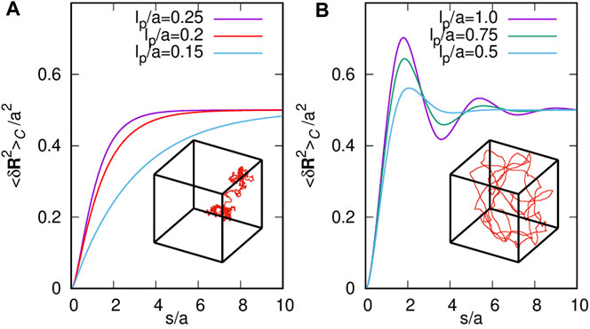
Let us remark that for any fixed value of a, the r.h.s of Eq. 31, as a function of L, shows the existence of a critical persistence length, ${\ell }_p^{\text{*}}=\sqrt{3}a/\left(2\pi \right)$ such that for all values of ${\ell }_p>{\ell }_p^{\text{*}}$, it exhibits an oscillating behavior, whereas for ${\ell }_p<{\ell }_p^{\text{*}}$, it is monotonically increasing. In Figure 1, we show the behavior of the mean-square end-to-end distance versus the length of the polymer for several values of the persistence length below and above ${\ell }_p^{\text{*}}$. Moreover, we also show sketches of conformational states corresponding to the monotonous and oscillating behaviors of the mean-square end-to-end distance. In addition, the same mathematical structure as the mean-square end-to-end distance found by Spakowitz and Wang [24] is noticeable for semiflexible polymers wrapping a spherical shell, and recently for semiflexible polymers confined to a square box [17].

FIGURE 1

FIGURE 1. Monotonous and oscillating behaviors of the mean-square end-to-end distance (Eq. 30) of polymers with ${\ell }_p$ below (A) and above (B) the critical persistence length ${\ell }_p^{\ast }=\sqrt{3}/\left(2\pi \right)a$ in cubic confinement. Inside the plotting area, we sketch the conformational states of each class of polymers.

4.2 Semiflexible Polymer Enclosed by a Spherical Surface

In this section, we provide results for the mean-square end-to-end distance for a semiflexible polymer enclosed inside of a spherical domain. All the problems are reduced to solve the Neumann eigenvalue problem $-{\nabla }^2\psi =\lambda \psi$ with Neumann boundary condition when the compact domain $\mathrm{ℬ}:=\left\{\mathbf{r}\in {\mathrm{ℝ}}^3:{\mathbf{r}}^2\le R^2\right\}$ is a center ball of radius R. This problem is widely studied in different mathematical physics problems [21, 23]. The eigenfunctions in this case can be given in terms of spherical Bessel functions $j_{\ell }\left(x\right)$ and spherical harmonic functions $Y_{\ell m}\left(\theta ,\phi \right)$:

${\psi }_{\ell mk}\left(r,\theta ,\phi \right)=N_{\ell k}{j}_{\ell }\left({\alpha }_{\ell k}\frac{r}{R}\right)Y_{\ell m}\left(\theta ,\phi \right),(32)$

where $r,\theta$, and φ are the standard spherical coordinates. The factor $N_{\ell k}$ is a normalization constant with respect to the volume of the ball $\mathrm{ℬ}$, given by

$N_{\ell k}=\frac{\sqrt{2}}{R^{3/2}}\frac{{\alpha }_{\ell k}}{j_{\ell }\left({\alpha }_{\ell k}\right){\left({\alpha }_{\ell k}^2-\ell \left(\ell +1\right)\right)}^{1/2}}.(33)$

The coefficients ${\alpha }_{\ell k}$ are the roots of $\partial j_{\ell }\left(x\right)/\partial x$, which, by using the identity $\ell j_{\ell -1}\left(x\right)-\left(\ell +1\right)j_{\ell +1}=\left(2\ell +1\right)\partial j_{\ell }\left(x\right)/\partial x$, satisfy the equation $\ell j_{\ell -1}\left({\alpha }_{\ell k}\right)=\left(\ell +1\right)j_{\ell +1}\left({\alpha }_{\ell k}\right)$. The eigenfunctions are enumerated by the collective index $\ell mk$, with $\ell =\mathrm{0,1,2},\cdots$ counting the order of spherical Bessel functions, $m=-\ell ,-\ell +1,\cdots ,\ell$, and $k=\mathrm{1,2,3},\cdots$ counting zeros. The eigenvalues of the Laplacian are given by ${\lambda }_{\ell mk}={\alpha }_{\ell k}^2/R^2$, which are independent of the numbers m. Now, we proceed to calculate ${\mathbf{r}}_{\ell mk}$ by using Eq. 26. It is enough to calculate $\underset{S^2}{{\displaystyle \mathrm{\oint }}}dS\mathbf{n}{Y}_{\ell m}\left(\theta ,\phi \right)$, since $\mathbf{n}\propto Y_{1m}$; thus, $\underset{S^2}{{\displaystyle \mathrm{\oint }}}dS\mathbf{n}{Y}_{1,\pm 1}\left(\theta ,\phi \right)=-\sqrt{\frac{2\pi }{3}}{R}^2\left(\pm 1,i,0\right)$ and $\underset{S^2}{{\displaystyle \mathrm{\oint }}}dS\mathbf{n}{Y}_{\mathrm{1,0}}\left(\theta ,\phi \right)=2\sqrt{\frac{\pi }{3}}{R}^2\left(\mathrm{0,0,1}\right)$. Now, we call ${\alpha }_{1k}:={\alpha }_k$; then, using Eq. 33 one has

${\mathbf{r}}_{1,\pm 1,k}=-2\sqrt{\frac{\pi }{3}}\frac{R^{5/2}}{{\alpha }_k{\left({\alpha }_k^2-2\right)}^{1/2}}\left(\pm 1,i,0\right),(34)$

${\mathbf{r}}_{\mathrm{1,0},k}=2\sqrt{\frac{2\pi }{3}}\frac{R^{1/2}}{{\alpha }_k{\left({\alpha }_k^2-2\right)}^{1/2}}\left(\mathrm{0,0,1}\right),(35)$

where roots $\left\{{\alpha }_k\right\}$ satisfy the equation $j_0\left({\alpha }_k\right)=2j_2\left({\alpha }_k\right)$. Using explicit functions of the spherical Bessel functions, the root condition is $F\left({\alpha }_k\right)=0$, where

$F\left(x\right)=\left(\frac{x^2}{2}-1\right)\sin x+x\cos x.(36)$

In the following, we use the general expression (Eq. 25) for the mean-square end-to-end distance. We calculate the mean-square end position, ${\sigma }^2\left(\mathbf{R}\right)=\frac{3}{5}{R}^2$, and use the factors ${\mathbf{r}}_{\ell mk}$; thus, the mean square end-to-end distance is

${\langle \delta {\mathbf{R}}^2\rangle }_{\mathrm{ℬ}}=\frac{6}{5}{R}^2-12R^2\stackrel{\infty }{{\displaystyle \sum }_{k=1}}\frac{1}{{\alpha }_k^2\left({\alpha }_k^2-2\right)}G\left(\frac{s}{2{\ell }_p},\frac{4}{3}{\left(\frac{{\ell }_p}{R}\right)}^2{\alpha }_k^2\right).(37)$

Following the same line of argument performed in [17], we observe numerically that $12{{{\displaystyle \sum }}^{\text{}}}_{k=1}^N\frac{1}{{\alpha }_k^2\left({\alpha }_k^2-2\right)}\to 6/5$ as N increases; this is consistent with Eq. 27. Thus, up to a numerical error ${10}^{-2}$, we claim that

$\begin{array}{c}\frac{{\langle \delta {\mathbf{R}}^2\rangle }_{\mathrm{ℬ}}}{R^2}\simeq \frac{6}{5}-\frac{6}{5}\text{exp}\left(-\frac{L}{2{\ell }_p}\right)\{\text{cosh}\left[\frac{L}{2{\ell }_p}{\left(1-\frac{4{\alpha }_1^2}{3}\frac{{\ell }_p^2}{R^2}\right)}^{\frac{1}{2}}\right]\\ +{\left(1-\frac{4{\alpha }_1^2}{3}\frac{{\ell }_p^2}{R^2}\right)}^{-\frac{1}{2}}\text{sinh}\left[\frac{L}{2{\ell }_p}{\left(1-\frac{4{\alpha }_1^2}{3}\frac{{\ell }_p^2}{R^2}\right)}^{\frac{1}{2}}\right]\}.\end{array}(38)$

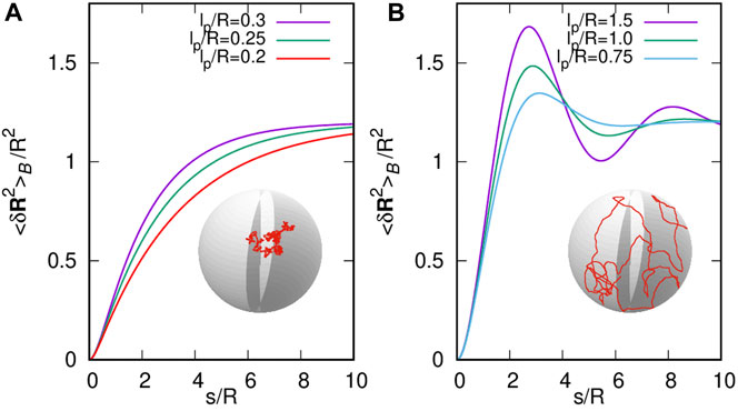
Let us remark that for any fixed value of R, the r.h.s of Eq. 38, as a function of L, shows the existence of a critical persistence length, ${\ell }_p^{\text{*}}=\sqrt{3}R/\left(2{\alpha }_1\right)$, with ${\alpha }_1\simeq 2.08158$ according to Eq. 36 such that for all values of ${\ell }_p>{\ell }_p^{\text{*}}$, it exhibits an oscillating behavior, whereas for ${\ell }_p<{\ell }_p^{\text{*}}$, it is monotonically increasing. In Figure 2, we show the behavior of the mean-square end-to-end distance versus the length of the polymer for several values of the persistence length below and above ${\ell }_p^{\text{*}}$. Moreover, we also show sketches of conformational states corresponding to the monotonous and oscillating behaviors of the mean-square end-to-end distance. In addition, it is noticeably that the same mathematical structure as the mean-square end-to-end distance found by Spakowitz and Wang [24] for semiflexible polymers wrapping a spherical shell, and recently for semiflexible polymers, confined to a square box [17].

FIGURE 2

FIGURE 2. Monotonous and oscillating behaviors of the mean-square end-to-end distance (Eq. 37) of polymers with ${\ell }_p$ below (A) and above (B) the critical persistence length ${\ell }_p^{\ast }=\sqrt{3}R/\left(2{\alpha }_1\right)$ in spherical confinement. Inside the plotting area, we sketch the conformational states of each class of polymers.

5 Concluding Remarks

In this work, we carry out an extension of the stochastic curvature formalism introduced in [17] to analyze the conformational states of a semiflexible polymer in a thermal bath for the cases when the polymer is in the open space ${\mathrm{ℝ}}^3$ and when it is in a bounded domain $\mathcal{D}\subset {\mathrm{ℝ}}^3$. The basic idea of formalism in the 3D case is followed by two postulates, that is, each conformational state corresponds to the realization of a path described by the stochastic Frenet–Serret Eq. 5a and Eq. 5b, to introduce a stochastic curvature vector $\mathit{k}\left(s\right)$, and a second postulate that gives the manner how $\mathit{\kappa }\left(s\right)$ is distributed according to the thermal fluctuations.

In the case of a polymer in an open space ${\mathrm{ℝ}}^3$, the standard Kratky–Porod formula for polymers is reproduced in three dimensions [16], while when the polymer is confined to a space bounded region $\mathcal{D}\subset {\mathrm{ℝ}}^3$, the conformational states show the existence of a critical persistence length ${\ell }_p^{\text{*}}$ such that for all values of ${\ell }_p>{\ell }_p^{\text{*}}$, the mean square distance from end to end exhibits an oscillating behavior, while for ${\ell }_p<{\ell }_p^{\text{*}}$, it exhibits a monotonic behavior in both cases of a cubic region and a spherical region. Furthermore, for each value of ${\ell }_p$, the function converges to twice the mean-square end position ${\sigma }^2\left(\mathbf{R}\right)$, that is, twice the variance of ${\mathbf{R}}^2$ with respect to the volume of the domain. The critical persistence length, therefore, distinguishes two conformational behaviors of the semiflexible polymer in the bound domain. On the one hand, polymers with persistence length below the critical value have a conformation similar to a Brownian random path. On the other hand, polymers with persistence length above the critical value adopt smooth conformations. In addition, it is highlighted that the mean-square end-to-end distance exhibits the same mathematical form for the discussed cases along with the manuscript (Eq. 31 and Eq. 38) and with the results reported for a polymer enclosed to a square box and rolling up a spherical surface [17, 24]. Nevertheless, the value difference of saturation and the critical persistence length reflect the particular geometric nature of the compact domain, including the dimensionality of the space. Note the particular mathematical expression in our work is due to the probability density function of the polymer’s ends, which is governed by a modified telegrapher equation. As a consequence of this resemblance, it can be concluded that the shape transition from oscillating to monotonous conformational states provides furthermore evidence of a universal signature for a semiflexible polymer enclosed in compact space.

Data Availability Statement

The original contributions presented in the study are included in the article/Supplementary Material, and further inquiries can be directed to the corresponding authors.

Author Contributions

Both authors contributed to the formulation of the method and the writing of the manuscript. JR contributed to the numerical analysis that provides the figures, while PC-V contributed to the mathematical calculations.

Conflict of Interest

The authors declare that the research was conducted in the absence of any commercial or financial relationships that could be construed as a potential conflict of interest.

Acknowledgments

PC-V and JR acknowledge financial support by Consejo de Ciencia y Tecnología del Estado de Puebla (CONCYTEP).

Footnotes

¹For the sake of notation, the dimension of the space in the persistence length definition is hidden. In those cases where an explicit dependence on the dimension is needed, it should be adequately scaled by the factor $2/\left(d-1\right)$.

References

1. Ronca S, “Polyethylene,” In Brydson’s Plastics Materials (8th ed.) (M Gilbert, ed.), pp. 247–78. Butterworth-Heinemann, 8th ed. ed., 2017. doi:10.1016/b978-0-323-35824-8.00010-4

CrossRef Full Text | Google Scholar

2. Wünsch J. Polystyrene: Synthesis, Production and Applications. RAPRA Technology Limited, Rapra Technology Limited (2000).

3. Cifra P, Bleha T. Shape Transition of Semi-flexible Macromolecules Confined in Channel and Cavity. Eur Phys J E (2010) 32(3):273–9. doi:10.1140/epje/i2010-10626-y

PubMed Abstract | CrossRef Full Text | Google Scholar

4. Locker CR, Harvey SC. A Model for Viral Genome Packing. Multiscale Model Simul (2006) 5(4):1264–79. doi:10.1137/060650684

CrossRef Full Text | Google Scholar

5. Köster S, Kierfeld J, Pfohl T. Characterization of Single Semiflexible Filaments under Geometric Constraints. Eur Phys J E (2008) 25(4):439–49. doi:10.1140/epje/i2007-10312-3

PubMed Abstract | CrossRef Full Text | Google Scholar

6. Reisner W, Morton KJ, Riehn R, Wang YM, Yu Z, Rosen M, et al. Statics and Dynamics of Single Dna Molecules Confined in Nanochannels. Phys Rev Lett (2005) 94:196101. doi:10.1103/physrevlett.94.196101

PubMed Abstract | CrossRef Full Text | Google Scholar

7. Benková Z, Rišpanová L, Cifra P. Structural Behavior of a Semiflexible Polymer Chain in an Array of Nanoposts. Polymers (2017) 9(8):313. doi:10.3390/polym9080313

CrossRef Full Text | Google Scholar

8. Saitô N, Takahashi K, Yunoki Y. The Statistical Mechanical Theory of Stiff Chains (1967).

9. Kleinert H, Chervyakov A. Perturbation Theory for Path Integrals of Stiff Polymers. J Phys A: Math Gen (2006) 39:8231–55. doi:10.1088/0305-4470/39/26/001

CrossRef Full Text | Google Scholar

10. Benetatos P, Frey E. Linear Response of a Grafted Semiflexible Polymer to a Uniform Force Field. Phys Rev E Stat Nonlin Soft Matter Phys (2004) 70:051806. doi:10.1103/PhysRevE.70.051806

PubMed Abstract | CrossRef Full Text | Google Scholar

11.Adsorption of polymers and polyelectrolytes. In Solid-Liquid Interfaces. In: J Lyklema, editor. Vol. 2 of Fundamentals of Interface and Colloid Science. Academic Press (1995). p. 5–1. – 5–100.

CrossRef Full Text | Google Scholar

12. Guven J, Vázquez-Montejo P. Confinement of Semiflexible Polymers. Phys Rev E Stat Nonlin Soft Matter Phys (2012) 85(2):026603–16. doi:10.1103/PhysRevE.85.026603

PubMed Abstract | CrossRef Full Text | Google Scholar

13. Guven J, María Valencia D, Vázquez-Montejo P. Environmental Bias and Elastic Curves on Surfaces. J Phys A: Math Theor (2014) 47(35). doi:10.1088/1751-8113/47/35/355201

CrossRef Full Text | Google Scholar

14. Spakowitz AJ, Wang ZG. End-to-end Distance Vector Distribution with Fixed End Orientations for the Wormlike Chain Model. Phys Rev E Stat Nonlin Soft Matter Phys (2005) 72:041802. doi:10.1103/PhysRevE.72.041802

PubMed Abstract | CrossRef Full Text | Google Scholar

15. Chen JZY. Theory of Wormlike Polymer Chains in Confinement. Prog Polym Sci (2016) 54-55:3–46. doi:10.1016/j.progpolymsci.2015.09.002

CrossRef Full Text | Google Scholar

16. Kratky O, Porod G. Röntgenuntersuchung Gelöster Fadenmoleküle. Recl Trav Chim Pays-bas (1949) 68(12):1106–22. doi:10.1002/recl.19490681203

CrossRef Full Text | Google Scholar

17. Castro-Villarreal P, Ramírez JE. Stochastic Curvature of Enclosed Semiflexible Polymers. Phys Rev E (2019) 100:012503. doi:10.1103/PhysRevE.100.012503

PubMed Abstract | CrossRef Full Text | Google Scholar

18. Montiel S, Ros A. Curves and Surfaces, Vol. 69. American Mathematical Soc. (2009).

19. Gardiner CW. Handbook of Stochastic Methods for Physics. Chem Nat Sci (1986) 25.

Google Scholar

20. Hermans JJ, Ullman R. The Statistics of Stiff Chains, with Applications to Light Scattering. Physica (1952) 18(11):951–71. doi:10.1016/s0031-8914(52)80231-9

CrossRef Full Text | Google Scholar

21. Feshbach H. Methods of Theoretical Physics. New York: McGraw-Hill (1953).

22. Chavel I. Eigenvalues in Riemannian Geometry, Vol. 115. Academic Press (1984).

23. Grebenkov DS, Nguyen B-T. Geometrical Structure of Laplacian Eigenfunctions. SIAM Rev (2013) 55(4):601–67. doi:10.1137/120880173

CrossRef Full Text | Google Scholar

24. Spakowitz AJ, Wang Z-G. Semiflexible Polymer Confined to a Spherical Surface. Phys Rev Lett (2003) 91:166102. doi:10.1103/physrevlett.91.166102

PubMed Abstract | CrossRef Full Text | Google Scholar