Elastography Validity Criteria Definition Using Numerical Simulations and MR Acquisitions on a Low-Cost Structured Phantom

MR Elastography is a novel technique enabling the quantification of mechanical properties in tissue with MRI. It relies on a three-step process that includes the generation of a mechanical vibration, motion capture using dedicated MR sequences, and data processing involving inversion algorithms. If not properly tuned to the targeted application, each of those steps may impact the final outcome, potentially causing diagnostic errors and thus eventually treatment mismanagement. Different approaches exist that account for acquisition or reconstruction errors, but simple tools and metrics for quality control shared by both developers and end-users are still missing. In this context, our goal is to provide an easily deployable workflow that uses generic validity criteria to assess the performance of a given MRE protocol, leveraging numerical simulations with an accessible experimental setup. Numerical simulations are used to help both determining sets of relevant acquisition parameters and assessing the data processing's robustness. Simple validity criteria were defined, and the overall pipeline was tested in a custom-built, structured phantom made of silicone-based material. The latter have the advantage of being inexpensive, easy to handle, facilitate the fabrication of complex structures which geometry resembles the anatomical structures of interest, and are longitudinally stable. In this work, we successfully tested and evaluated the overall performances of our entire MR Elastography pipeline using easy-to-implement and accessible tools that could ultimately translate in MRE standardized and cost-effective procedures.

Introduction

Magnetic Resonance Elastography (MRE) non-invasively assesses and quantifies mechanical properties of tissue in vivo [1, 2]. Various MRE techniques have been developed, involving the combination of interdependent processes (mechanical vibration generation, motion-sensitized MR sequences, image processing algorithms) all of which may impact the qualitative and quantitative outcomes. As a result, MRE, despite being available for decades, has not entered clinical routine application yet; a consensus on precision and accuracy of this technique still needs to be defined. Indeed, one of the major drawbacks of MRE is the lack of a gold-standard that could enable to compare elastograms with each other. Rheometry may provide a reference measurement of bulk mechanical properties of various materials [3–7], but the precision of common rheometers or dynamic mechanical analysis (DMA) systems depend on multiple factors, like the type of instrument used or the sample's size and experimental environment [6, 8, 9]. Furthermore, performing reliable rheometry over a range of frequencies comparable with those employed in MRE may not be possible with common rheometers and specific high-frequency measurement systems may be required [8, 9]. In addition, biomechanical properties of ex vivo tissue specimens that lack perfusion are very different than those of perfused in vivo body parts, making a direct comparison between classical rheometers and MRE difficult. In this context, biases and errors intrinsic to the technique should be assessed and controlled to avoid the generation (and further the interpretation) of unreliable elastograms. Since MRE relies on the encoding of the tissue displacement into the phase of the complex MR signal, metrics that take into account phase errors are good candidates to measure raw data quality. Phase-to-noise ratio (PNR) can be used to evaluate the impact of noise on the reconstructed displacement. Given that the phase standard deviation in radians is equal to the inverse of the magnitude SNR [10], PNR is proportional to both the SNR and the encoded phase shift. PNR can be computed in numerous ways, either by including the specific details of a given experiment [11] or independently of them, but at the expense of extra acquisitions [12]. Displacement-to-noise ratio (DNR) has been similarly used as a metric, either by exploiting the knowledge of the encoding sequence details and SNR [13], or by estimating a motion SNR from the displacement noise [14, 15]. The octahedral shear strain (OSS) and the derived OSS-SNR have been introduced as indicators of reconstruction accuracy showing better performance than the motion SNR [15]. However, OSS is obtained from spatial derivatives of the motion field, which makes it dependent on the processing [16]. The ratio of local shear wavelength λ to pixel size a has also been introduced as an indicator of reconstruction accuracy [17, 18], and values were reported for different methods [19, 20]. From these studies, the range of optimal λ/a appears to be broad (~5–20), although best performances are generally achieved in the range 6.7–10, especially at low SNR.

Numerical simulations can be used as a validation tool by generating displacement fields (forward problem) for given boundary conditions, visco-elasticity distributions, and vibration sources. The displacement fields are then fed into the MRE reconstruction pipeline, which solves the inverse problem and retrieves the mechanical properties for comparison with ground-truth values. Simulations are generally based on analytical formulations [5, 14, 17, 21] or finite element methods (FEM), either with custom-developed tools [22–24] or dedicated commercial softwares [20, 24–30]. Simulations are very useful to assess the error linked to reconstruction algorithms, however they do not suffice to reflect all potential limitations of an MRE experiment (transducer, B₀ and B₁ inhomogeneities, SNR, motion sensitivity, susceptibility issues, and heterogeneity of the material at very small scales). Validation is thus typically obtained from self-made or commercial phantoms mimicking biological tissues, which shape and properties depend on a targeted application. A thorough overview of materials used for ultrasound elastography is given in [31], and here we will focus on those commonly used in MRE. Water-based phantoms are largely spread and include natural or synthetic polymers. Natural polymers comprise gelatin-based phantoms, easy to make, that are characterized by a linearly elastic behavior, low viscosity and frequency dependency [32]. However, they are sensitive to temperature changes [33] and also to the fabrication process [27, 34, 35]. Agar can be used alone [1, 2, 5, 20, 36, 37] or added to gelatin [38] with a multi-step heating and cooling procedure at precise temperature steps. Over a period of about 1 year post fabrication, such phantoms have shown a general decrease of storage modulus following an initial increase phase (1–5 months). Synthetic polymers like polyvinyl alcohol cryogels (PVA) are obtained by performing repeated cycles of freezing and thawing of boiled and stirred PVA solutions. Their mechanical properties depend both on the number of cycles and the PVA concentration [14, 39–42]. This fabrication process enables phantoms with anisotropic mechanical properties [21], yet inhomogeneous temperature changes within the entire volume cause inhomogeneities leading to uneven inclusion-background interfaces [39, 43]. Commercially available phantoms (CIRS Inc., USA), made from patented Zerdine hydrogel, are more expensive than water-based phantoms [44]. They contain well-defined inclusions but are essentially non-viscous and the measured values often differ from those declared by the manufacturer [19, 20, 45–48]. Polyvinyl chloride (PVC, also known as plastisol) phantoms are fabricated by heating-up a mixture of PVC and a softening agent to high temperatures (160–177°C) while constantly stirring before pouring into a heat-resistant mold [8, 49]. Arunachalam and colleagues have assumed that a 90-day period was sufficient to reach stable mechanical properties [9]. They also reported weak MR signal and very low loss moduli of the material, causing increased reflections. Finally, silicone has been used for Digital Image Elasto-Tomography (DIET) [50, 51], and for mechanical imaging using pressure sensors [52], but little so far for MRE [53, 54]. Compared to the other materials described above, silicone simplifies considerably the phantom fabrication process. Typically, silicones are created by mixing two components, and the final stiffness can be controlled by the addition of a softener or hardener. Besides, many silicones are room temperature vulcanizing (RTV), which eases the fabrication process and enables the realization of homogenous structures with smooth interfaces.

Our objective is to establish simple and easily transferable validity criteria, setting the ground for basic procedures in MRE quality control and efficient deployment of the technique in the clinics. In the presented work, we assess the limitations of MRE for a given protocol, comparing reconstruction performance from both fully simulated and acquired datasets in a low-cost silicone-based phantom.

Materials and Methods

Sample Preparation and Phantom Fabrication

Different samples were obtained by mixing the two components of a silicone rubber (Eurosil 4 A+B, Schouten SynTec, the Netherlands) together with an oil softener (Eurosil Softener, Schouten SynTec, the Netherlands). An empirical density of 1,000 kg/m³ yielded accurate volume estimation of the final material. The silicone components were stirred manually (1–5 min depending on total volume) in a plastic container until a homogeneous mixture was obtained. Different stiffness properties were obtained by fixing the weight ratio between the silicone bi-components (A and B) and varying the softener composition, expressed as 1A : 1B : Sx. For rheological measurements, silicone mixtures were poured into small cylindrical plastic containers (diameter 25 mm) to create seven samples of about 6 mm height, with softener compositions of S1.0, S1.5, S1.7, S1.9, S2.1, S2.3, and S2.5. All samples were made on the same day.

An MRE phantom was made that consisted of four cylindrical inclusions of various diameter in a homogeneous, rectangular background (Figure 1). The silicone mixture for the background (1A : 1B : S1.9) was first poured into a 3D-printed mold (Fortus 450 m, Stratasys, USA) with 4 removable 3D printed cylinders (Figure 1A). As the 3D print may produce rough surfaces, which promotes the formation of micro air bubbles while pouring uncured silicone, a plastic sheet was placed to cover the inner surface of the mold (Figure 1B). Furthermore, an aerosol release agent (Pol-Ease 2500, Schouten SynTec, Netherlands) was applied on the surface of the cylinders to facilitate the extraction of the phantom from the mold. We allowed the silicone to fully cure for 1 day before extracting the cylindrical inserts, and filled the remaining volume with a softer mixture 1A : 1B : S2.1 to create the inclusions. The final size of the phantom was 182 × 108 × 90 mm³ with inclusions of diameter 10, 20, 30, and 40 mm referred to as I1, I2, I3, I4 according to their size. All samples were stored away from direct light at room temperature, in a closed plastic container together with a two-way humidity control bag (“Humidipak,” D'Addario, USA) to ensure 45–50% humidity.

FIGURE 1

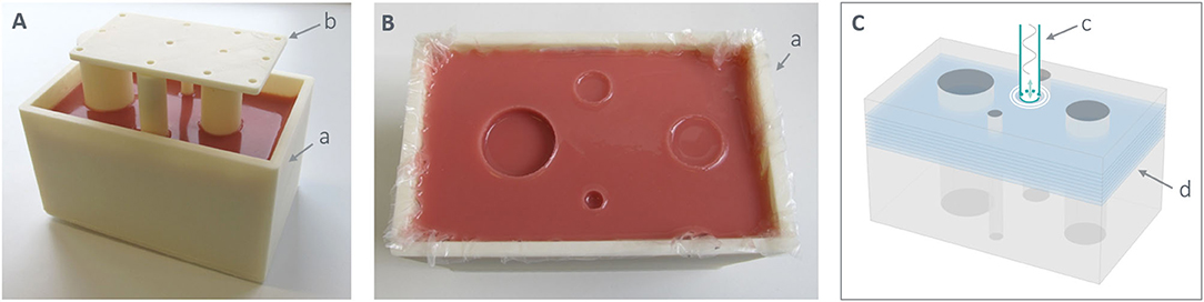
Figure 1. MRE silicone phantom. (A) Example of the fabrication process of the background with the four cylinders positioned by means of an aligning lid (b). (B) Picture of the silicone phantom with four cylindrical inclusions in the 3D-printed rectangular mold (a). (C) 3D design of the phantom with the four inclusions that shows the position of the vibration source (c) at its surface as well as the location of the acquired or exported nine slices (in blue) in the case of (3 mm)³ voxel size (d).

Silicone Stability

Stability over time of the prepared seven cylindrical silicone samples was investigated using a rotational rheometer (MCR series, 302 and 702, Anton Paar, Austria) to extract their complex shear modulus G^* = G' + iG” (G': storage modulus, G”: loss modulus). For each measurement, the upper rotating plate (flat model PP25) which diameter is identical to the samples, was positioned with an automatic set point of 5-N normal force to enable a sufficient compression and rotation. A sweep of the shear strain amplitude in the range 0.01–10% was performed at 10 Hz to verify the linear behavior of each material. Subsequently, a shear strain amplitude of 1% was used for G^* measurement with a linear frequency sweep from 100 to 1 Hz. For each sample, two consecutive measurements of the frequency sweep were acquired. The same measurements were repeated at several time points, respectively at 1, 2, 4, 7, 15, and 22 weeks post fabrication.

An example of the frequency sweep measurement obtained with the silicone samples is given in Supplementary Figure 1. An increased standard deviation for the two consecutive measurements can be observed for frequencies >20 Hz (Supplementary Figure 1A). Similarly, larger G” than G' are observed above 35–40 Hz, even though the material kept its solid structure. Therefore, we assumed that the measurements corresponding to 10 Hz provided reliable information and we used those values to evaluate the sample stability over time.

Simulations

Forward Problem

Numerical simulations were performed using COMSOL Multiphysics 5.4 (COMSOL AB, Sweden). The geometry of the simulated phantom was defined as a rectangular solid with dimensions identical to the MRE silicone phantom described above, including the same four cylindrical inclusions (Figure 1C). The vibration area was defined as a circular region of 16 mm diameter on the front face of the phantom, at half distance between I3 and I4, similarly to the physical vibration setup used later.

For the simulation's physics definition, the Solid Mechanics interface from the Structural Mechanics module was used. The front face of the phantom was set as a “Free” boundary, while all the other faces were assigned to a “Fixed Constraint” node to reproduce the condition of the containing mold. A “Prescribed Displacement” node was assigned to the vibration area with an imposed sinusoidal displacement perpendicular to the surface with a 200-μm amplitude and frequency f_vib of 57 Hz. For both types of regions (background and inclusions) the material properties were defined using a “Linear Elastic Material” domain node with a “Viscoelasticity” domain, without any particular contact definition between the two materials.

In order to define G^* = G' + iG” of the different regions, we employed an isotropic Standard Linear Solid model (see Supplementary Material). The simulation consisted in a “Time Dependent” study over a time interval of 12 vibration periods T = 1/f_vib, sufficient for the waves to propagate in the whole volume, with a time step equal to T/20, for a total simulation time of 41 min (Intel Xeon CPU E5-2680 v4 @ 2.4 GHz, 14 cores, RAM 128 GB). The exported simulated data consisted in the displacement field components u, v, w (in X, Y, and Z direction, respectively) at time points tau = i^*T/N (with N the number of wave phases sampled during MRE acquisitions, five in this case) of the last vibration period. A spatial grid of 9 contiguous axial slices was defined for three different isotropic voxel sizes of 2.5, 3.0, and 3.5 mm³, respectively. The central slice (i.e. slice 5) was set at 22 mm from the surface (Figure 1C).

Synthetic MR Data

Displacement field components were converted into synthetic complex MRE data via a custom MATLAB (R2020a, The MathWorks Inc., USA) script. Phase-encoding was artificially achieved by multiplying the displacement data by the fractional encoding factor (Equation 1 from [12]) of the MRE encoding scheme, with a motion-encoding-gradient (MEG) of 54 mT/m:

$\begin{array}{l}\phi =\gamma u{\displaystyle {\int }_0^{TR}}MEG(t)sin(2\pi f_{vib}t)dt\\ =\frac{\gamma A_{MEG}u}{f_{MEG}}\frac{sin(\pi q)}{\pi (1-q^2)}\\ \text{with }q=\frac{f_{vib}}{f_{MEG}}\\ \text{when MEG}(t)=A_{MEG}sin(2\pi f_{MEG}t)& (1)\end{array}$

with φ the vibration-encoded phase, γ the gyromagnetic ratio, u and f_vib the amplitude and frequency of the vibration at a given coordinate in space, A_MEG and f_MEG the amplitude and frequency of the sinusoidal motion encoding gradient MEG(t). Magnitude of the synthetic data was arbitrarily set to one everywhere. Since a reference dataset without MEG is required for our reconstruction, a separate dataset was generated with identical geometry, magnitude set to 1 and phase to 0 everywhere (no additional noise was considered).

MR Imaging

MRE was performed on a clinical 3 T Magnetom Prisma scanner (Siemens Healthineers, Germany) using a fractional encoding gradient-echo sequence [12] and a 20-channel head coil. To constrain the bulk motion, the phantom was kept inside its plastic mold. The accessible phantom face was oriented parallel to the axial plane of the scanner. A custom vibration system was used, similar to the ones described in [42, 55]. The latter consists of a loudspeaker (12NW100-8, B&C Speakers, Italy) and a waveguide (flexible, 16-mm diameter plastic tubing, Tecnotubi Picena, Italy) which circular opening was positioned in contact at the surface of the phantom. A vibration frequency of 57 Hz was used that corresponded to one of the resonant frequencies of the waveguide (calibrated separately). The vibration was produced via a wave generator (33500B Trueform, Keysight, USA) coupled to an audio amplifier (XLS 1502, Crown, USA). The MRE sequence encoded five time points of the vibration phases with a four-point scheme, acquiring three motion-encoded data series (each for one of the three spatial MEG directions) and a reference series (without motion encoding). Three experiments were performed at different spatial resolutions with the following acquisition parameters: MEG amplitude 54 mT/m, TE/TR 12.3/180 ms, acquisition matrix 96 × 54, 9 contiguous axial slices, isotropic voxel size of 2.5, 3.0, and 3.5 mm³, MEG frequency of 105.26, 104.39, and 104.39 Hz, respectively, as summarized in Table 1. The central slice was positioned at about 1/4 of the phantom's height, i.e. at around 22 mm from the surface. The scans were scheduled with time points identical to the rheometric measurements run in the silicone samples, plus 1 day.

TABLE 1

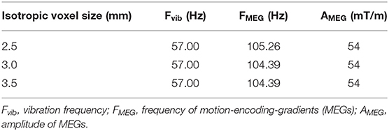
Table 1. Motion encoding parameters used for MRE acquisitions on the phantom for different voxel sizes.

In each MRE session, relaxation times T₁ and T₂ of the phantom were also quantified (see Supplementary Material).

Data Processing and Analysis

MRE Reconstruction

Both the synthetic and experimental raw MRE data were processed using a custom software performing a 3D curl-based direct inversion [12]. All the elastograms were then exported for further processing using MATLAB scripts. In this paper we focus only on G', the MRE output information most commonly used by numerous research groups.

A mask was drawn manually around the phantom boundaries before unwrapping the phase data. Since the reconstruction software requires to calculate multiple spatial derivatives, the generated elastograms are by default cropped by two voxels in 3D with respect to the initially defined volume of interest (VOI). In addition, we chose to discard two more pixels for each slice in order to take into account possible calculation error propagation that often translates in G' underestimation at boundaries. Elastograms of the five central slices were used for the analysis of synthetic data. Alternatively, elastograms of the three central slices were used with experimental data as more discrepancy was observed on surrounding slices.

Regions of Interest (ROIs)

For synthetic data, maps of the G parameter were exported at the same coordinates as the displacement field data, in order to obtain a map of the inclusion positions on the same spatial interpolation grid. This way, ROIs were automatically available for the location of the inclusions inside the background. For the experimental data, ROIs were defined as circles centered in the inclusions, segmented from T₂ maps. The respective masks were co-registered with the MRE datasets. To avoid partial volume effects due to the larger voxel sizes employed in MRE, the mask for the background was eroded by two voxels surrounding the inclusions. Mean, median, and standard deviation values of G' were calculated within the different ROIs. All the segmentation steps were based on data quality considerations detailed below.

MRE Validity Criteria

In order to evaluate the quality and reliability of raw MRE data, simple metrics were chosen, easily transposable to any MRE method. In particular, SNR was calculated voxel-wise for each set of raw data and converted into phase and displacement amplitude uncertainty maps using Equation 1. The mean SNR and standard deviation of the reference dataset (acquired without motion encoding gradients) were used to discard voxels with low SNR and therefore large phase error on final MRE maps. This threshold was empirically set to 2 standard deviations below the mean SNR: voxels on the elastograms were discarded when at least one dataset of the three encoded directions did not have a sufficient SNR. Additionally, due to derivative calculations on the reconstructed data, we discarded two more voxels on each side of the voxels excluded by the SNR threshold by dilating the SNR mask in all three directions.

To calculate the ratio of shear wavelength λ to voxel size a for the three resolutions, λ was estimated via Equation 2 [56]:

$\begin{array}{ll}\begin{array}{c}\lambda =\frac{1}{{\text{f}}_{\text{vib}}}\sqrt{\frac{{\text{G}}^{\prime }}{\rho }}\\ \end{array}& (2)\end{array}$

where f_vib is the vibration frequency of 57 Hz, ρ the density of the material (assumed to be 1,000 kg/m³), and G' is the estimated storage modulus. For G' values, we considered the median values obtained with the 3-mm resolution within the background (silicone softener composition S1.9) and within the largest inclusion I4 (silicone softener composition S2.1).

MRE Validation

Reconstruction algorithms can have an impact both on the calculated stiffness and the apparent objects geometry. To validate the MRE pipeline, the contrast-to-noise ratio CNR_i between the i-th inclusion and the background [19, 20, 57, 58] was calculated using Equation 3:

$\begin{array}{ll}\begin{array}{c}CN{R}_i=\frac{2{(m_i-m_B)}^2}{{\sigma }_i^2+{\sigma }_B^2}\\ \end{array}& (3)\end{array}$

where m_i, m_B are the mean values of G' within the i-th inclusion and the background, and σ_i, σ_B are the corresponding standard deviations of G'. Here, the median was used instead of the mean to allow for non-Gaussian distributions.

Root-mean-square-error RMSE was calculated for the voxels in the different regions according to Equation 4:

$\begin{array}{ll}\begin{array}{c}RMSE=\sqrt{\frac{1}{N}{\displaystyle {\sum }_j^N\frac{{({G^{\prime }}_j-{G^{\prime }}_{0,j})}^2}{{G^{\prime }}_{0,j}{}^2}}}\end{array}& (4)\end{array}$

where $G_{0,j}^{\prime }$ is the storage modulus defined in the simulation and $G_j^{\prime }$ is the reconstructed value in a voxel j. For MRE data, $G_{0,j}^{\prime }$ in the background was taken as the median value at 3 mm resolution, whereas $G_{0,j}^{\prime }$ values in the inclusions were estimated as $G_{0,j}^{\prime }$ in the background divided by the ratio $G_{S1.9}^{\prime }/G_{S2.1}^{\prime }$ measured via rheometry.

Statistical Analyses

For each considered resolution, the probability distribution was tested using the Kolmogorov-Smirnov method. Differences between G' values in the inclusions and those in the background were assessed with the Kruskal-Wallis test (α = 0.05), followed by a Mann-Whitney test for the two-by-two comparisons between the four inclusions and the background. The significance level was adjusted for multiple comparisons using the Bonferroni correction, and a p-value of 0.0125 was considered as significant.

Results

Silicone Stability

Figure 2 summarizes the evolution over time of G' measured at 10 Hz for all samples, showing an initial variation of the material properties leading to good stability after 2–4 weeks post fabrication. The increase in G' never exceeds 1.1 kPa for all samples, except in the case of softener composition S1.0 where the variation almost equals 2 kPa. In addition, the silicone samples exhibit, as expected, a clear distinction in terms of G^* values, with higher values in the case of lower softener proportion (Figure 2).

FIGURE 2

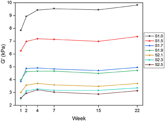
Figure 2. Rheometry measurements at different timepoints (weeks post fabrication) of the complex shear modulus component G' at 10 Hz angular frequency for all the silicone samples prepared with various softener compositions.

Simulations

Analysis of the reconstructed elastograms for the simulated phantom is shown in Figure 3. As described above, the reconstruction does not provide any value within a 2-voxel rim around the object. The inclusions are circled in red and the sections (A-A and B-B) show G' values across the five central slices (Figure 3A).

FIGURE 3

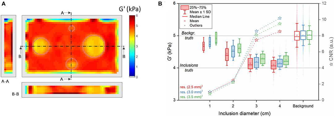
Figure 3. Reconstructed component G' of the complex shear modulus obtained from simulated data. (A) Example of a reconstructed 3D dataset at the central slice and its sections along the indicated lines A-A and B-B at 3-mm resolution (red circles: true position of the inclusions). (B) Summary of the values in all reconstructed voxels (over five slices) of the different segmented regions (inclusions I1, I2, I3, I4 and background) for all three considered voxel sizes (red: (2.5 mm)³, blue: (3.0 mm)³, green: (3.5 mm)³). The upper and lower edges of the boxes in the boxplot represent, respectively the first and the third quartile levels; horizontal line within the boxes: median value; square: mean value; whiskers: mean ± 1 standard deviation; outliers are indicated as dots. The horizontal lines across the plot represent the values set in the simulation for the different regions (see Table 2). Stars: contrast-to-noise ratio CNR between each inclusion and the background.

Despite having identical compositions, large inclusions, compared to small ones, are better discriminated from the background even though they all showed significant differences (p < 0.0125) at all resolutions (see boxplots in Figure 3B). This trend is confirmed by the CNR values, greater in the inclusions I4 and I3 than in I2 and I1. The reconstruction software yields more accurate values in the background and in I4 and I3 than in I2 and I1, close to the ground-truth defined in the simulation (Figure 4). In fact, the error is similar in the background and in the inclusions I4 and I3, while it increases more than 2-fold for the smaller inclusions I2 and I1. In general, Figures 3, 4 indicate that a smaller voxel size corresponds to a greater standard deviation of G' within each region and to a larger error in the background.

FIGURE 4

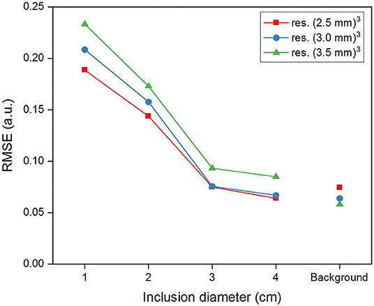
Figure 4. Root-mean-square-error (RMSE) of G' reconstructed within the inclusions and in the background for the simulated data and for the different spatial resolutions.

The wavelength-to-voxel size ratios λ/a are calculated for each spatial resolution and summarized in Table 2. This ratio decreases with increasing voxel size, with all values included between 10 and 15.7.

TABLE 2

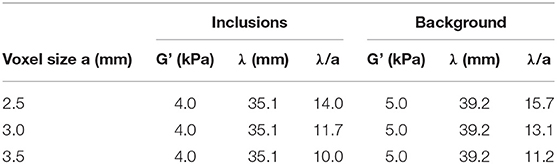
Table 2. Simulated values of G' in the inclusions and background with corresponding shear wavelength λ and the calculated ratio of wavelength to voxel size λ/a for the considered values of a.

Phantom MRI and MRE

The employed phantom fabrication technique produced cylindrical shapes with sharp contours and overall proper adherence between the different silicone regions at the inclusions boundaries (cf. Figure 1). The values of both T₁ and T₂ of the two silicone compositions differ by <10 ms, with minor variations over time post fabrication (Supplementary Figure 2). The inclusions shape and position were identified on T₂ maps, which presented less B₁ inhomogeneity at the center of the phantom than T₁ maps (Supplementary Figure 3), and were thus used for ROI segmentation.

The SNR and the error values both on the MR phase and the corresponding displacement amplitude are reported in Table 3. These errors were rather small and did not contribute in the overall data thresholding. An example of the reconstructed G' maps is represented in Figure 5 for the central slice at week 4 post fabrication. The number of voxels near the edges of the phantom with underestimated values of G' is between 2 and 5 voxels greater than what is observed in synthetic data. In general, the voxels discarded by our SNR threshold are located near the boundaries of the phantom and at its center, in correspondence with partial volume effects and the location of the vibration source.

TABLE 3

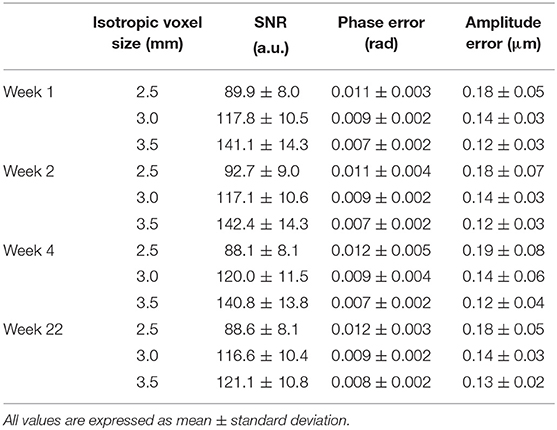
Table 3. Calculated SNR and corresponding phase and amplitude errors within the phantom for the MRE datasets at different resolutions and measurement timepoints post fabrication.

FIGURE 5

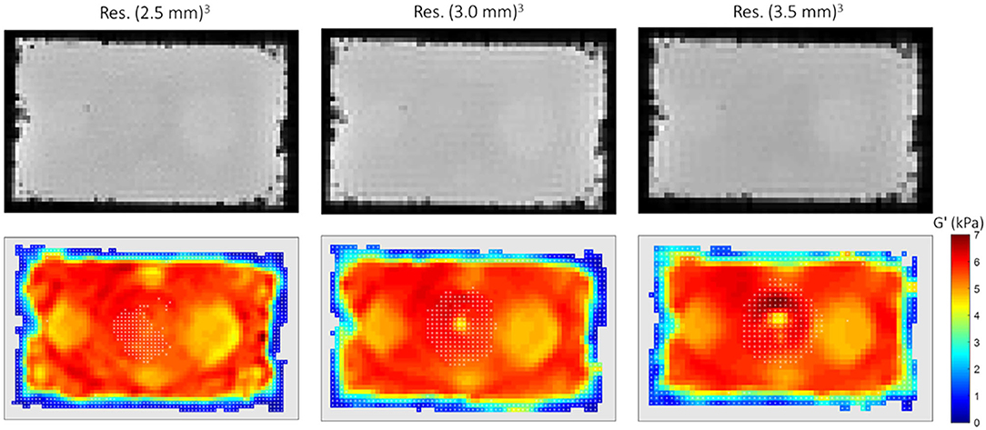
Figure 5. MRE results at week 4 post fabrication for different resolutions (from left to right: (2.5 mm)³, (3.0 mm)³, (3.5 mm)³). Top row: magnitude of the reference dataset in the 5th slice. Bottom row: corresponding G' maps with phantom's contours being masked (light gray) and white cross hatches indicating the voxels discarded based on the SNR threshold.

Figure 6 presents the reconstructed G' values in the segmented regions of the phantom at week 4 post fabrication. As observed with synthetic data, the standard deviation within a given region decreases with increasing voxel size, and the values within the inclusions stand out of the background more clearly while inclusion size increases. This effect led to a higher CNR for the largest inclusions although CNR values in the phantom were smaller than those obtained from simulated data. As in synthetic data, G' in all the inclusions and for all the resolutions was significantly different from the background's (p < 0.0125). As expected, the background silicone with a lower softener content of S1.9 has greater storage modulus values than the inclusions made with a softener composition of S2.1. The mean values in the background are however lower than their median, because of the skewed G' distribution and the contribution of underestimated voxels near the phantom's edges.

FIGURE 6

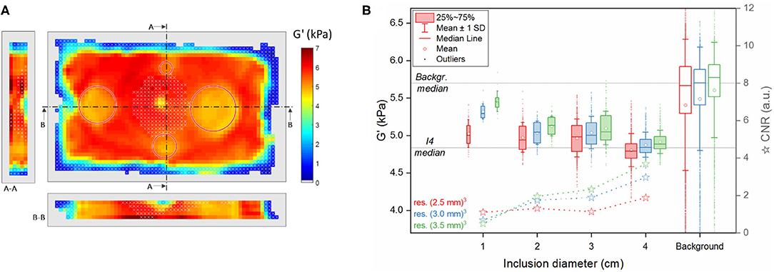
Figure 6. MRE results 4 weeks after fabrication. (A) Example of a reconstructed 3D dataset at the central slice and its sections along the indicated lines A-A and B-B at 3-mm resolution (red circles: position of the inclusions). (B) Summary of G' values in the reconstructed voxels of the three middle slices in the different segmented regions (inclusions I1, I2, I3, I4 and background) and for the three acquired voxel sizes (red: (2.5 mm)³, blue: (3.0 mm)³, green: (3.5 mm)³). The upper and lower edges of the boxes in the boxplot represent, respectively the first and the third quartile levels; horizontal line within the boxes: median value; square: mean value; whiskers: mean ± 1 standard deviation; outliers are indicated as dots. The horizontal lines across the plot represent the median values measured at 3 mm resolution in the background and in the inclusion I4 (G'_b = 5.7 kPa, G'_I4 = 4.8 kPa, respectively). Stars: contrast-to-noise ratio CNR between each inclusion and the background.

The RMSE values for G' measured via MRE in the different regions for each considered resolution are illustrated in Figure 7. The error is smallest for the inclusion I4, and largest for I1, with all values greater than observed for synthetic data. As for simulations, we observed an increased error in the background for the finest resolution, as opposed to the inclusions where the errors increased with increasing voxel size.

FIGURE 7

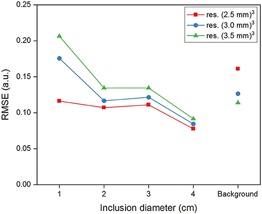
Figure 7. Root-mean-square-error (RMSE) of G' reconstructed within the inclusions and in the background for MRE data at different spatial resolutions.

The evolution of G' values over time (Figure 8) shows a higher initial variation than in the case of the rheometry samples, with stability reached at around 4-weeks post fabrication. Furthermore, ratios of G' between the two silicone compositions S1.9 and S2.1 measured via MRE are similar to those measured via rotational rheometry. The wavelength-to-voxel size ratios λ/a estimated from MRE data are summarized in Table 4. This ratio increases over time for all the regions following the initial stiffening of the silicone material, with λ/a values ranging from 9.7 and 17.1.

FIGURE 8

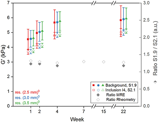
Figure 8. Plot of G' median values measured via MRE in the background (filled symbols) and in the inclusion I4 (empty symbols) vs. time post fabrication and with error bars representing the standard deviation for the three resolutions (red (2.5 mm)³, blue (3.0 mm)³, green (3.5 mm)³). Right axis: ratio of G' between background and inclusion for 3 mm resolution (gray filled diamonds) and between corresponding samples for rheometry (gray empty diamonds).

TABLE 4

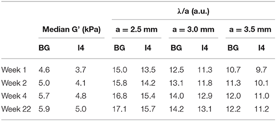
Table 4. Measured G' in the largest inclusion (I4, softener composition S2.1) and background (BG, softener composition S1.9) at 3-mm resolution for different time elapsed since fabrication and corresponding estimated ratio of wavelength to voxel size λ/a for the considered voxel sizes a.

Discussion

Silicone Based Phantoms for MRE

The proposed silicone-based preparation shows great promise as a low-cost, easy-to-reproduce, and durable option for quality control and calibration in MRE experiments.

Rheometry monitoring of the complex shear modulus showed good long-term stability after a 2- to 4-week delay, across all prepared samples. During this initial phase, an overall initial stiffening of maximum 1.6 kPa was observed. Remarkably, despite the exceeding of the maximum recommended softener composition from the manufacturer, our results showed that G' could be changed and remained stable over time. From this, we obtained a range of realistic stiffnesses covering G' values from 2 to 10 kPa, similar to that observed in biological tissues.

The fabricated MRE silicone phantom exhibited similar evolution of G' over time, while maintaining its G' ratios (background/inclusions) (Figure 8). Yet, the overall variations in G' measured with MRE (~1.3 kPa) were generally larger than G' obtained with rheometry (~0.7 kPa). This may be caused by variations in the aging process due to their size differences. Furthermore, such differences may also be expected since rheometry is not a gold standard and operates in a different frequency regime compared to MRE. Nevertheless, our results indicate that rheometry is a good candidate to provide an estimation of the expected values measured via MRE and consists in a good basis for fine-tuning future phantom preparations.

Here, we used two silicone compositions and a simple geometry for the purpose of the study. With appropriate modifications to our fabrication procedure, it should be possible to create more complex, multilayer geometries or anatomically-shaped features in an easy way by exploiting the good shape conservation and interface contact between silicone mixtures once cured. A potential difficulty in the fabrication process may arise from the formation of micro air bubbles. Gradually pouring the silicone over a plastic sheet covering the internal faces of the mold helped mitigating this problem, yet some susceptibility artifacts due to air bubbles at the edges of the inclusions (see Figure 5 in the proximity of I3) remained. To solve this issue, one can envision either using materials with smooth and solid surfaces for all the molding parts, such as PMMA or silicone molds with anti-adherent coating [59], scanners with lower magnetic field strengths, or a vacuum chamber for degassing during the fabrication process. Viscosity is another important aspect of the silicone material, and in our case it was greater than what is reported for other commonly used MRE phantoms. As biological tissue, our samples exhibit a dispersive behavior (Supplementary Figures 1A,B). The subsequent wave attenuation has the advantage to prevent successive reflections at boundaries and hence the presence of standing waves especially in small objects but may prevent from obtaining sufficient wave propagation inside large objects.

Finally, our results showed T₁ and T₂ values in the order of 1,030 ms and 240 ms, respectively, for both compartments of the MRE phantom (differences never exceeded 7.2 ms for both T₁ and T₂), and with little variation over time (overall <0.9 and 2.9% in relative terms). Further studies may consider tuning the silicone relaxation times by the addition of paramagnetic substances compatible with the silicone mixture during fabrication. This would help further the sequence optimization for a faster transfer to in vivo application, in particular when other markers than stiffness are required for segmentation for example [59].

Simulations

We showed that synthetic MRE data produced via numerical simulations can be used with our reconstruction pipeline. The obtained elastograms displayed distinct (and expected) differences in G' values between the defined inclusions and the background. By varying voxel size, we could investigate the resolvability of the latter inclusions as a function of their size, as well as the accuracy of the reconstruction algorithm. It was possible to accurately retrieve G' values within large homogeneous regions while observing some limitations for inclusions smaller than 3-cm diameter. For larger voxel size and/or for a smaller inclusion diameter, our results showed a decreased standard deviation of G' as well as an overestimation of G' within the inclusions. Both findings may be partly explained by the local homogeneity assumption made in the inversion algorithm, and by the calculation of the derivatives within a local neighborhood. With large voxel sizes or small inclusions, more voxels are affected by the discontinuity in the distribution of the mechanical properties at the inclusion boundaries. The higher dispersion, especially visible in the background region when using small voxel sizes, can be explained by a sub-optimal λ/a ratio. The theoretical λ/a for the 2.5-mm resolution belongs to the higher end of the suggested optimal interval of 5–20 found in the literature. Furthermore, for this same resolution (data not shown), G' maps exhibit inhomogeneities that match the wave propagation pattern and ultimately lead to larger RMSE in the background. Considering that our simulations do not add any noise and ensure that no standing waves occur, one can conclude that such effects are exclusively due to the reconstruction pipeline and that large λ/a ratios should be avoided. All together, these results suggest that numerical simulations can provide a reliable prediction of reconstructed results for different experimental conditions in a simple, yet heterogeneous object. Possible challenges in designing accurate simulations of more complex geometries lie in the difficulties of realistic modeling, in particular of the boundary conditions and wave propagation at the various interfaces. Although simulations of a body organ may require a detailed knowledge of mechanical properties and their distribution at a fine spatial scale, their feasibility may be increased from the availability of structural datasets acquired via different imaging techniques (MRI, CT) in combination with appropriate, simplified physical assumptions. Finally, we believe that simulations could help improving the overall MRE performances by tuning either the MRE parameters, or by addressing specific aspects of the reconstruction pipeline. In this study we chose one single frequency and three spatial resolutions, but simulations can easily be performed using various frequencies and a large span of spatial resolutions.

MRE Experiments

Overall, experimental results appear very similar to the reconstructed simulation data (Figures 3, 5, 6). Some differences can be seen on the edges of the phantom exhibiting uneven contours and susceptibility artifacts at the air-silicone interface. Like the simulations, MRE demonstrated good accuracy for retrieving G' across large, homogeneous regions (background, I4, and I3), and limitations for inclusions smaller than 3 cm diameter. Those limitations are tied to the specific MRE protocol chosen in this study. We chose a vibration frequency of 57 Hz in the range commonly used in human studies for various diseases, both focal and diffuse (e.g. in the brain, breast, liver, muscle, prostate, heart), along with acquisition times that ensure patient comfort. Yet, if required, mapping smaller objects with confidence could be achieved by improving the inversion algorithm, in particular by assuming anisotropy and medium heterogeneity. Further development in the experimental protocol could also help in that direction and provide more accurate MRE results, typically by adapting the mechanical vibration settings along with the acquisition parameters or using a retrospective data resampling [60]. We also noticed biases introduced by the reconstruction process, such as the underestimation of G' values near the boundaries of the phantom (Figure 5) or the greater error in the background at the finest resolution (Figure 7). That said, confidence in the estimation of errors from the MRE side must be balanced with the fact that RMSE calculation requires an actual ground truth, here estimated from the simulation data.

Validity Criteria for MRE

The λ/a ratio was always in the range suggested by the literature, gradually increasing with time from the initial stiffening phase in our phantom. Interestingly, we note (Table 4) that a relatively small change in voxel size (e.g. 3 mm vs. 2.5 mm) affects the ratio λ/a more than an increase in G' of almost 1.2 kPa, as could be measured from week 1 to week 4. Therefore, if decimation or interpolation of voxels are always possible after the acquisition, an appropriate native resolution remains essential for relevant reconstruction outcomes. More concretely, it shows that the quest for finer resolutions does reach a limit where it starts to impede MRE performance rather than improving it.

In our study, we used a fixed vibration frequency along with a variable resolution conversely to most studies that investigated the λ/a ratio by employing a wide range of vibration frequencies and a fixed pixel size. The range of chosen resolutions may not be sufficient to define the optimal λ/a ratio but is sufficient to show how much it impacts reconstruction, without being influenced by wave penetration or motion efficiency. Although this approach may lead to smoothing effects from filtering kernels in the processing of the raw MRE data, it is more relevant for mono-frequency MRE approaches and in organs where wave attenuation may vary significantly in a small range of frequencies.

Considering SNR, the computed values over time were high (Table 3) and translated into rather small phase and amplitude errors, defeating their relevance to discard unreliable voxels. In a more general case, however, phase uncertainty may be used to eliminate regions where the encoding of the vibration produces a net phase lower than the corresponding error. This may occur because of low SNR, either due to short ${\text{T}}_2^{*}$ in general, a strong vibration, highly attenuated wave amplitude or insufficient encoding efficiency. It is particularly important to be able to distinguish the two latter conditions since a lack of waves may be due to physical properties or transducer settings, whereas the encoding efficiency may be improved acting on the sequence parameters. The motion encoding efficiency, however, is not always available to the end-user, and providing this information in terms of encoded radians per displacement at the scanner user interface would allow useful data quality considerations and an estimation of PNR. Using SNR only as a thresholding metric, on the other hand, was successfully applied. In our study, it appeared particularly useful in regions where large motion amplitudes led to strong losses of MR signal, i.e. in voxels near the transducer location. Such a metric is simple and has the advantage of not requiring knowledge of the sequence details. We strongly recommend to systematically calculate the SNR and to use it as a basic quality control check to prevent any potential diagnostic errors that will in turn lead to inadequate patient treatment.

Conclusions

The proposed work presents an effective and adaptable solution for testing, assessing, or comparing MRE methods performances, which is summarized in Figure 9. Synthetic MRE was successfully obtained from simulated displacement fields. We demonstrated the fabrication of a simple, low-cost, structured MRE phantom with controlled mechanical properties close to biological tissue that are stable over time, replicating the ground-truth phantom modeled in our simulations. Furthermore, the material is quite dispersive and hence suitable for studying multi-frequency MRE. Such a phantom can be easily adapted to various applications and deployed worldwide to study the performance of a given MRE experiment and reconstruction pipeline. Our simulations successfully matched experimental MRE results on the phantom. Similar results, trends, and limitations regarding the accuracy of both G' values and the inclusion shape were observed. As a consequence, simulations can be used to predict or estimate performance in MRE experiments in silico and showcase the possible intrinsic method limitations. This step could be cost and time effective for parameters fine tuning in anticipation of the optimization phases at the scanner. Finally, we showed how the interpretation of the reconstructed maps can be improved by discarding unreliable voxels. In particular, besides phase uncertainty based criteria which may be useful in certain cases and the importance of λ/a ratio, an SNR-based discrimination should be applied in general for direct thresholding to discard unreliable elastogram regions.

FIGURE 9

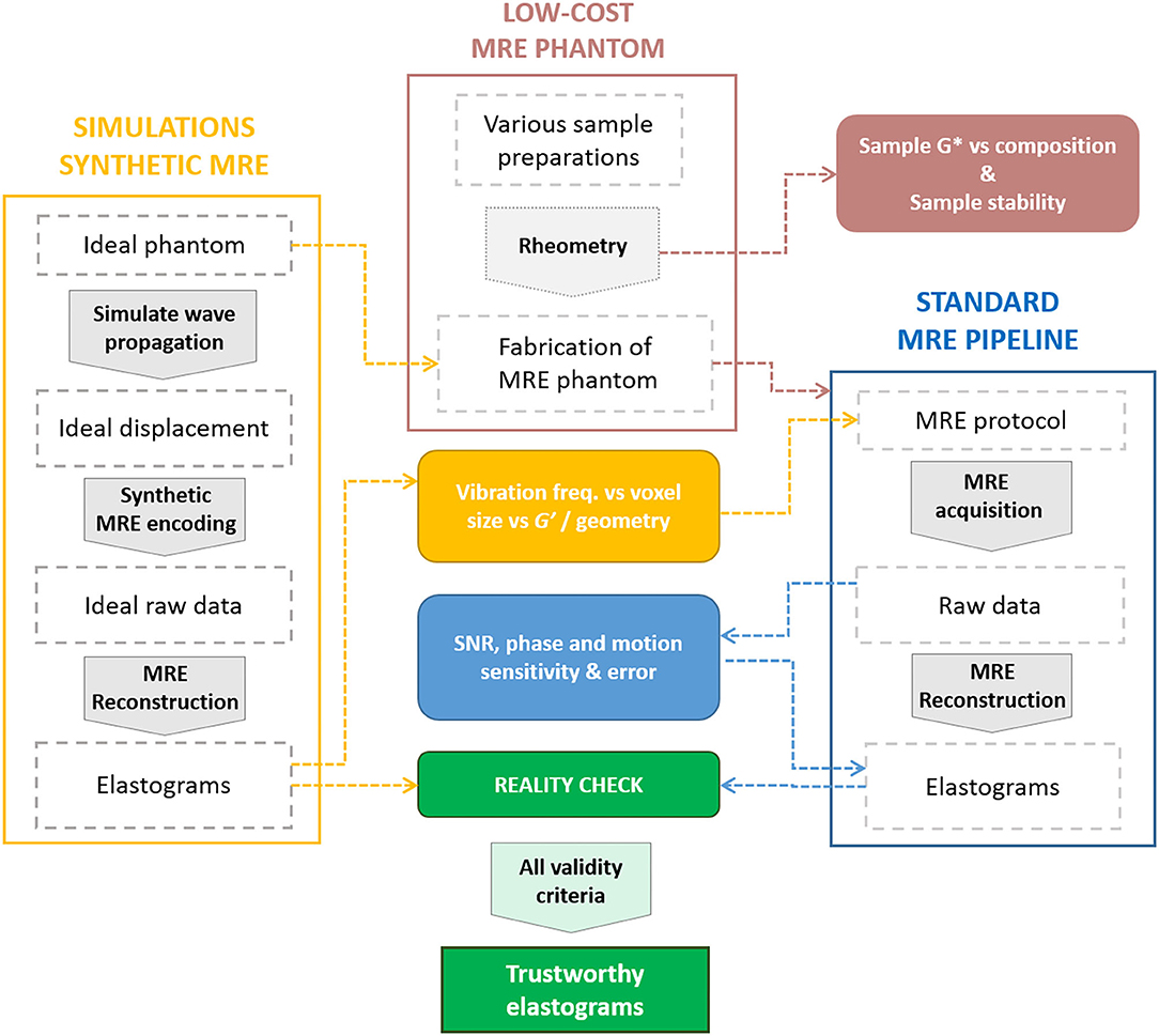
Figure 9. Diagram summarizing our pipeline for MRE validation using simulations (yellow), a low-cost silicone phantom (pink), MRE experiments (blue) and the relationships between different steps (arrows). Steps are represented as dashed frames, processes as large arrows, and outputs as filled boxes.

Data Availability Statement

The raw data supporting the conclusions of this article will be made available by the authors, without undue reservation.

Author Contributions

MY, MS, JW, and NS: study design. MY: simulations. MY, MA, and NS: experiments. MY, MS, RS, and NS: data analysis. All authors contributed to writing and proofreading the manuscript.

Funding

This work was supported by Horizon 2020 European Research Council (668039), Swiss National Science Foundation (170575), and the Swiss State Secretariat for Education, Research and Innovation (15.0341-1).

Conflict of Interest

The authors declare that the research was conducted in the absence of any commercial or financial relationships that could be construed as a potential conflict of interest.

Acknowledgments

We would like to express our gratitude to Dr. Olivier Braissant for his precious support in phantom preparation.

Supplementary Material

The Supplementary Material for this article can be found online at: https://www.frontiersin.org/articles/10.3389/fphy.2021.620331/full#supplementary-material

References

1. Muthupillai R, Lomas D, Rossman P, Greenleaf J, Manduca A, Ehman R. Magnetic resonance elastography by direct visualization of propagating acoustic strain waves. Science. (1995) 269:1854–7. doi: 10.1126/science.7569924

PubMed Abstract | CrossRef Full Text | Google Scholar

2. Plewes DB, Betty I, Urchuk SN, Soutar I. Visualizing tissue compliance with MR imaging. J Magn Reson Imaging. (1995) 5:733–8. doi: 10.1002/jmri.1880050620

PubMed Abstract | CrossRef Full Text | Google Scholar

3. Vappou J, Breton E, Choquet P, Goetz C, Willinger R, Constantinesco A. Magnetic resonance elastography compared with rotational rheometry for in vitro brain tissue viscoelasticity measurement. Magn Reson Mater Phys Biol Med. (2007) 20:273–8. doi: 10.1007/s10334-007-0098-7

PubMed Abstract | CrossRef Full Text | Google Scholar

4. Doyley MM, Weaver JB, Van Houten EEW, Kennedy FE, Paulsen KD. Thresholds for detecting and characterizing focal lesions using steady-state MR elastography. Med Phys. (2003) 30:495–504. doi: 10.1118/1.1556607

PubMed Abstract | CrossRef Full Text | Google Scholar

5. Papazoglou S, Hirsch S, Braun J, Sack I. Multifrequency inversion in magnetic resonance elastography. Phys Med Biol. (2012) 57:2329–46. doi: 10.1088/0031-9155/57/8/2329

PubMed Abstract | CrossRef Full Text | Google Scholar

6. Dittmann F, Hirsch S, Tzschätzsch H, Guo J, Braun J, Sack I. In vivo wideband multifrequency MR elastography of the human brain and liver. Magn Reson Med. (2016) 76:1116–26. doi: 10.1002/mrm.26006

PubMed Abstract | CrossRef Full Text | Google Scholar

7. Klatt D, Friedrich C, Korth Y, Vogt R, Braun J, Sack I. Viscoelastic properties of liver measured by oscillatory rheometry and multifrequency magnetic resonance elastography. Biorheology. (2010) 47:133–41. doi: 10.3233/BIR-2010-0565

PubMed Abstract | CrossRef Full Text | Google Scholar

8. Lefebvre PM, Koon KTV, Brusseau E, Nicolle S, Palieme JF, Lambert SA, et al. Comparison of viscoelastic property characterization of plastisol phantoms with magnetic resonance elastography and high-frequency rheometry. Proc Annu Int Conf IEEE Eng Med Biol Soc EMBS. (2016) 2016:1216–9. doi: 10.1109/EMBC.2016.7590924

PubMed Abstract | CrossRef Full Text | Google Scholar

9. Arunachalam SP, Rossman PJ, Arani A, Lake DS, Glaser KJ, Trzasko JD, et al. Quantitative 3D magnetic resonance elastography: comparison with dynamic mechanical analysis. Magn Reson Med. (2017) 77:1184–92. doi: 10.1002/mrm.26207

PubMed Abstract | CrossRef Full Text | Google Scholar

10. Brown RW, Cheng Y-CN, Haacke EM, Thompson MR, Venkatesan R. Magnetic Resonance Imaging: Physical Principles and Sequence Design, Second Edition. Chichester, UK: John Wiley & Sons Ltd (2014). doi: 10.1002/9781118633953

CrossRef Full Text

11. Rump J, Klatt D, Braun J, Warmuth C, Sack I. Fractional encoding of harmonic motions in MR elastography. Magn Reson Med. (2007) 57:388–95. doi: 10.1002/mrm.21152

PubMed Abstract | CrossRef Full Text | Google Scholar

12. Garteiser P, Sahebjavaher RS, Ter Beek LC, Salcudean S, Vilgrain V, Van Beers BE, et al. Rapid acquisition of multifrequency, multislice and multidirectional MR elastography data with a fractionally encoded gradient echo sequence. NMR Biomed. (2013) 26:1326–35. doi: 10.1002/nbm.2958

PubMed Abstract | CrossRef Full Text | Google Scholar

13. Guenthner C, Runge JH, Sinkus R, Kozerke S. Analysis and improvement of motion encoding in magnetic resonance elastography. NMR Biomed. (2018) 31:e3908. doi: 10.1002/nbm.3908

PubMed Abstract | CrossRef Full Text | Google Scholar

14. Sinkus R, Tanter M, Catheline S, Lorenzen J, Kuhl C, Sondermann E, et al. Imaging anisotropic and viscous properties of breast tissue by magnetic resonance-elastography. Magn Reson Med. (2005) 53:372–87. doi: 10.1002/mrm.20355

PubMed Abstract | CrossRef Full Text | Google Scholar

15. McGarry MDJ, Van Houten EEW, Perriez PR, Pattison AJ, Weaver JB, Paulsen KD. An octahedral shear strain-based measure of SNR for 3D MR elastography. Phys Med Biol. (2011) 56:152–64. doi: 10.1088/0031-9155/56/13/N02

PubMed Abstract | CrossRef Full Text | Google Scholar

16. Guenthner C, Kozerke S. Encoding and readout strategies in magnetic resonance elastography. NMR Biomed. (2018) 31:e3919. doi: 10.1002/nbm.3919

PubMed Abstract | CrossRef Full Text | Google Scholar

17. Yue JL, Tardieu M, Julea F, Boucneau T, Sinkus R, Pellot-Barakat C, et al. Acquisition and reconstruction conditions in silico for accurate and precise magnetic resonance elastography. Phys Med Biol. (2017) 62:8655–70. doi: 10.1088/1361-6560/aa9164

PubMed Abstract | CrossRef Full Text | Google Scholar

18. Papazoglou S, Hamhaber U, Braun J, Sack I. Algebraic Helmholtz inversion in planar magnetic resonance elastography. Phys Med Biol. (2008) 53:3147–58. doi: 10.1088/0031-9155/53/12/005

PubMed Abstract | CrossRef Full Text | Google Scholar

19. Honarvar M, Rohling R, Salcudean SE. A comparison of direct and iterative finite element inversion techniques in dynamic elastography. Phys Med Biol. (2016) 61:3026–48. doi: 10.1088/0031-9155/61/8/3026

PubMed Abstract | CrossRef Full Text | Google Scholar

20. Honarvar M, Sahebjavaher RS, Rohling R, Salcudean SE. A Comparison of finite element-based inversion algorithms, local frequency estimation, and direct inversion approach used in MRE. IEEE Trans Med Imaging. (2017) 36:1686–98. doi: 10.1109/TMI.2017.2686388

PubMed Abstract | CrossRef Full Text | Google Scholar

21. Chatelin S, Charpentier I, Corbin N, Meylheuc L, Vappou J. An automatic differentiation-based gradient method for inversion of the shear wave equation in magnetic resonance elastography: specific application in fibrous soft tissues. Phys Med Biol. (2016) 61:5000–19. doi: 10.1088/0031-9155/61/13/5000

PubMed Abstract | CrossRef Full Text | Google Scholar

22. McGarry M, Johnson CL, Sutton BP, Van Houten EE, Georgiadis JG, Weaver JB, et al. Including spatial information in nonlinear inversion MR elastography using soft prior regularization. IEEE Trans Med Imaging. (2013) 32:1901–9. doi: 10.1109/TMI.2013.2268978

PubMed Abstract | CrossRef Full Text | Google Scholar

23. Sinkus R, Lorenzen J, Schrader D, Lorenzen M, Dargatz M, Holz D. High-resolution tensor MR elastography for breast tumour detection. Phys Med Biol. (2000) 45:1649–64. doi: 10.1088/0031-9155/45/6/317

PubMed Abstract | CrossRef Full Text | Google Scholar

24. Bilasse M, Chatelin S, Altmeyer G, Marouf A, Vappou J, Charpentier I. A 2D finite element model for shear wave propagation in biological soft tissues: application to magnetic resonance elastography. Int J Numer Method Biomed Eng. (2018) 34:1–19. doi: 10.1002/cnm.3102

PubMed Abstract | CrossRef Full Text | Google Scholar

25. Barnhill E, Nikolova M, Ariyurek C, Dittmann F, Braun J, Sack I. Fast robust dejitter and interslice discontinuity removal in MRI phase acquisitions: application to magnetic resonance elastography. IEEE Trans Med Imaging. (2019) 38:1578–87. doi: 10.1109/TMI.2019.2893369

PubMed Abstract | CrossRef Full Text | Google Scholar

26. Honarvar M, Sahebjavaher R, Sinkus R, Rohling R, Salcudean SE. Curl-based finite element reconstruction of the shear modulus without assuming local homogeneity: time harmonic case. IEEE Trans Med Imaging. (2013) 32:2189–99. doi: 10.1109/TMI.2013.2276060

PubMed Abstract | CrossRef Full Text | Google Scholar

27. Atay SM, Kroenke CD, Sabet A, Bayly PV. Measurement of the dynamic shear modulus of mouse brain tissue in vivo by magnetic resonance elastography. J Biomech Eng. (2008) 130:21013. doi: 10.1115/1.2899575

CrossRef Full Text | Google Scholar

28. Barnhill E, Davies PJ, Ariyurek C, Fehlner A, Braun J, Sack I. Heterogeneous Multifrequency Direct Inversion (HMDI) for magnetic resonance elastography with application to a clinical brain exam. Med Image Anal. (2018) 46:180–8. doi: 10.1016/j.media.2018.03.003

PubMed Abstract | CrossRef Full Text | Google Scholar

29. Thomas-Seale LEJ, Klatt D, Pankaj P, Roberts N, Sack I, Hoskins PR. A simulation of the magnetic resonance elastography steady state wave response through idealised atherosclerotic plaques. IAENG Int J Comput Sci. (2011) 38:394–400.

Google Scholar

30. Manduca A, Rossman TL, Lake DS, Glaser KJ, Arani A, Arunachalam SP, et al. Waveguide effects and implications for cardiac magnetic resonance elastography: a finite element study. NMR Biomed. (2018) 31:6–8. doi: 10.1002/nbm.3996

PubMed Abstract | CrossRef Full Text | Google Scholar

31. Cao Y, Li GY, Zhang X, Liu YL. Tissue-mimicking materials for elastography phantoms: a review. Extrem Mech Lett. (2017) 17:62–70. doi: 10.1016/j.eml.2017.09.009

CrossRef Full Text | Google Scholar

32. Doyley MM, Perreard I, Patterson AJ, Weaver JB, Paulsen KM. The performance of steady-state harmonic magnetic resonance elastography when applied to viscoelastic materials. Med Phys. (2010) 37:3970–9. doi: 10.1118/1.3454738

PubMed Abstract | CrossRef Full Text | Google Scholar

33. Okamoto RJ, Clayton EH, Bayly PV. Viscoelastic properties of soft gels: comparison of magnetic resonance elastography and dynamic shear testing in the shear wave regime. Phys Med Biol. (2011) 56:6379–400. doi: 10.1088/0031-9155/56/19/014

PubMed Abstract | CrossRef Full Text | Google Scholar

34. Gordon-Wylie SW, Solamen LM, McGarry MDJ, Zeng W, VanHouten E, Gilbert G, et al. MR elastography at 1 Hz of gelatin phantoms using 3D or 4D acquisition. J Magn Reson. (2018) 296:112–20. doi: 10.1016/j.jmr.2018.08.012

PubMed Abstract | CrossRef Full Text | Google Scholar

35. Solamen LM, Gordon-Wylie SW, McGarry MD, Weaver JB, Paulsen KD. Phantom evaluations of low frequency MR elastography. Phys Med Biol. (2019) 64:065010. doi: 10.1088/1361-6560/ab0290

PubMed Abstract | CrossRef Full Text | Google Scholar

36. Huwart L, Peeters F, Sinkus R, Annet L, Salameh N, ter Beek LC, et al. Liver fibrosis: Non-invasive assessment with MR elastography. NMR Biomed. (2006) 19:173–9. doi: 10.1002/nbm.1030

PubMed Abstract | CrossRef Full Text | Google Scholar

37. Bigot M, Chauveau F, Amaz C, Sinkus R, Beuf O, Lambert SA. The apparent mechanical effect of isolated amyloid-β and α-synuclein aggregates revealed by multi-frequency MRE. NMR Biomed. (2020) 33:1–10. doi: 10.1002/nbm.4174

PubMed Abstract | CrossRef Full Text | Google Scholar

38. Madsen EL, Hobson MA, Shi H, Varghese T, Frank GR. Tissue-mimicking agar/gelatin materials for use in heterogeneous elastography phantoms. Phys Med Biol. (2005) 50:5597–618. doi: 10.1088/0031-9155/50/23/013

PubMed Abstract | CrossRef Full Text | Google Scholar

39. Chu KC, Rutt BK. Polyvinyl alcohol cryogel: an ideal phantom material for MR studies of arterial flow and elasticity. Magn Reson Med. (1997) 37:314–9. doi: 10.1002/mrm.1910370230

PubMed Abstract | CrossRef Full Text | Google Scholar

40. Capilnasiu A, Hadjicharalambous M, Fovargue D, Patel D, Holub O, Bilston L, et al. Magnetic resonance elastography in nonlinear viscoelastic materials under load. Biomech Model Mechanobiol. (2019) 18:111–35. doi: 10.1007/s10237-018-1072-1

PubMed Abstract | CrossRef Full Text | Google Scholar

41. Surry KJM, Austin HJB, Fenster A, Peters TM. Poly(vinyl alcohol) cryogel phantoms for use in ultrasound and MR imaging. Phys Med Biol. (2004) 49:5529–46. doi: 10.1088/0031-9155/49/24/009

PubMed Abstract | CrossRef Full Text | Google Scholar

42. Salameh N, Sarracanie M, Armstrong BD, Rosen MS, Comment A. Overhauser-enhanced magnetic resonance elastography. NMR Biomed. (2016) 29:607–13. doi: 10.1002/nbm.3499

CrossRef Full Text | Google Scholar

43. Madsen EL, Hobson MA, Frank GR, Shi H, Jiang J, Hall TJ, et al. Anthropomorphic breast phantoms for testing elastography systems. Ultrasound Med Biol. (2006) 32:857–74. doi: 10.1016/j.ultrasmedbio.2006.02.1428

PubMed Abstract | CrossRef Full Text | Google Scholar

44. Oudry J, Bastard C, Miette V, Willinger R, Sandrin L. Copolymer-in-oil phantom materials for elastography. Ultrasound Med Biol. (2009) 35:1185–97. doi: 10.1016/j.ultrasmedbio.2009.01.012

PubMed Abstract | CrossRef Full Text | Google Scholar

45. Baghani A, Salcudean S, Honarvar M, Sahebjavaher RS, Rohling R, Sinkus R. Travelling wave expansion: a model fitting approach to the inverse problem of elasticity reconstruction. IEEE Trans Med Imaging. (2011) 30:1555–65. doi: 10.1109/TMI.2011.2131674

PubMed Abstract | CrossRef Full Text | Google Scholar

46. Fovargue D, Kozerke S, Sinkus R, Nordsletten D. Robust MR elastography stiffness quantification using a localized divergence free finite element reconstruction. Med Image Anal. (2018) 44:126–42. doi: 10.1016/j.media.2017.12.005

PubMed Abstract | CrossRef Full Text | Google Scholar

47. Sahebjavaher RS, Frew S, Bylinskii A, ter Beek L, Garteiser P, Honarvar M, et al. Prostate MR elastography with transperineal electromagnetic actuation and a fast fractionally encoded steady-state gradient echo sequence. NMR Biomed. (2014) 27:784–94. doi: 10.1002/nbm.3118

PubMed Abstract | CrossRef Full Text | Google Scholar

48. Chami L, Yue JL, Lucidarme O, Lefort M, Pellot-Barakat C. Feasibility of liver shear wave elastography with different transducers. IEEE Int Ultrason Symp IUS. (2016) 2016:1–4. doi: 10.1109/ULTSYM.2016.7728400

CrossRef Full Text | Google Scholar

49. Leclerc GE, Debernard L, Foucart F, Robert L, Pelletier KM, Charleux F, et al. Characterization of a hyper-viscoelastic phantom mimicking biological soft tissue using an abdominal pneumatic driver with magnetic resonance elastography (MRE). J Biomech. (2012) 45:952–7. doi: 10.1016/j.jbiomech.2012.01.017

PubMed Abstract | CrossRef Full Text | Google Scholar

50. Peters A, Chase GJ, Van Houten EEW. Digital image elasto-tomography: mechanical property estimation of silicone phantoms. Med Biol Eng Comput. (2008) 46:205–12. doi: 10.1007/s11517-007-0275-x

PubMed Abstract | CrossRef Full Text | Google Scholar

51. Peters A, Chase JG, Houten EEW. Estimating elasticity in heterogeneous phantoms using Digital Image Elasto-Tomography. Med Biol Eng Comput. (2009) 47:67–76. doi: 10.1007/s11517-008-0368-1

PubMed Abstract | CrossRef Full Text | Google Scholar

52. Egorov V, Sarvazyan AP. Mechanical imaging of the breast. IEEE Trans Med Imaging. (2008) 27:1275–87. doi: 10.1109/TMI.2008.922192

CrossRef Full Text | Google Scholar

53. Kashif AS, Lotz TF, Mcgarry MD, Pattison AJ. Silicone breast phantoms for elastographic imaging evaluation. Am Assoc Phys Med. (2013) 40:063503. doi: 10.1118/1.4805096

PubMed Abstract | CrossRef Full Text | Google Scholar

54. Solamen LM, McGarry MD, Tan L, Weaver JB, Paulsen KD. Phantom evaluations of nonlinear inversion MR elastography. Phys Med Biol. (2018) 63:145021. doi: 10.1088/1361-6560/aacb08

PubMed Abstract | CrossRef Full Text | Google Scholar

55. Maître X, Lamain E, Sinkus R, Louis B, Darrasse L. Whole brain MRE with guided pressure waves. Proc Intl Soc Mag Reson Med. (2011) 21:3489.

56. Hirsch S, Braun J, Sack I. Magnetic Resonance Elastography. Weinheim, Germany: Wiley-VCH Verlag GmbH & Co. KGaA (2016). doi: 10.1002/9783527696017

CrossRef Full Text | Google Scholar

57. Doyley MM, Feng Q, Weaver JB, Paulsen KD. Performance analysis of steady-state harmonic elastography. Phys Med Biol. (2007) 52:2657. doi: 10.1088/0031-9155/52/10/002

PubMed Abstract | CrossRef Full Text | Google Scholar

58. Bilgen M. Target detectability in acoustic elastography. IEEE Trans Ultrason Ferroelectr Freq Control. (1999) 46:1128–33. doi: 10.1109/58.796118

CrossRef Full Text | Google Scholar

59. Altermatt A, Santini F, Deligianni X, Magon S, Sprenger T, Kappos L, et al. Design and construction of an innovative brain phantom prototype for MRI. Magn Reson Med. (2019) 81:1165–71. doi: 10.1002/mrm.27464

PubMed Abstract | CrossRef Full Text | Google Scholar

60. Andoh F, Yue JL, Julea F, Tardieu M, Noûs C, Page G, et al. Multi-frequency MRE for elasticity quantitation and optimal tissue discrimination: a two-platform liver fibrosis mimicking phantom study. NMR Biomed. (2021).