On the Comparative Suitability of Strain Relaxation and Stress Relaxation Compression for Ultrasound Poroelastic Tissue Characterization

Poroelastic tissue strain imaging measures the time-varying and spatially varying deformation of a soft-tissue matrix during compression as the tissue fluid flows out of the compartmental boundaries. With the help of ultrasound, it has been carried out by observing the evolution of the images of the ultrasound echo strain over time, which shows that, in a stress-relaxation experiment (constantly applied global axial strain), a front of negative dilatation (volumetric strain) propagates slowly from the boundaries of a sample toward the center of the compressed region. The fitting of equations that predict this behavior to experimental data has earlier allowed quantitative imaging of the product of aggregate modulus and permeability of a tissue phantom, H_Ak, and its Poisson's ratio, ν. An ability to image and measure such novel tissue characteristics is likely to benefit biomedical research and have a wide range of clinical applications, including the assessment of lymphoedema, the diagnosis of cancer, the prediction of anticancer drug effectiveness, and monitoring of the tissue response to various treatments. This method is problematic, however, for application in vivo because the calculation of the volumetric strain requires the lateral and elevational strains, which are not easily measured accurately with conventional ultrasound strain imaging. This paper investigates for the first time whether the ultrasound observation in a strain-relaxation experiment (constantly applied uniaxial stress) could be used to observe the same mechanical behavior and provide the same information about the properties of a poroelastic sample as in a stress-relaxation experiment. The analytical theory was used to demonstrate that the propagation of dilatation shown in stress relaxation should also be observable in strain relaxation and that it should be detectable using axial strain, which is relatively easily measured in vivo. Finite element modeling (FEM) was employed to simulate all strain components within a homogeneous poroelastic material first during strain relaxation and then during stress relaxation, again demonstrating their equivalence for the observation of the propagation of a dilatation. The validity of using the strain relaxation conditions as an alternative to stress relaxation for measuring a poroelastic material's response was further confirmed by a fitting of the analytical models to the results of FEM. This allowed for an inversion of the time-varying volumetric strain, to recover the images of H_Ak and ν, for either loading configuration. The strain-relaxation configuration offers not only an opportunity to derive the same important quantitative poroelastic properties of the tissue as stress relaxation but also the potential to avoid the difficulties and errors associated with the estimation of strain along the axes perpendicular to the imaging axis, thus offering opportunities for easier clinical translation.

Introduction

Tissue physiology [1, 2] and the nature of the time-dependent response to a sustained compression [3, 4] both indicate that soft tissue is poroelastic. Poroelastic strain imaging measures the time-varying and spatially varying deformation of the elastic matrix as the tissue fluid flows out of the compressed region of any soft tissue that is subjected to sustained compression. Ultrasound tracking of the images of the echo strain over time shows that, when a constant axial strain is applied on the tissue, the dilatation (volumetric strain) decreases slowly from the boundaries of a sample toward its center. An ability to image and measure such a tissue behavior is likely to have diverse clinical applications, including the assessment of lymphoedema, the diagnosis of cancer, and the monitoring of the tissue response to various treatments.

Soft tissue is multiphase in nature. As a result, in contrast to linear viscoelastic models, poroelastic models describe more closely the deformation that soft tissue experiences when subjected to a sustained compressive force. The resulting local volume reduction (equal to the amount of fluid that has been forced away from the compressed volume [5]) allows the spatially varying and time-varying strain to be related to particular biomechanical properties, namely the permeability k, Poisson's ratio v, and Young's modulus E, that describe the microstructure of a poroelastic material. For practical measurement and imaging, ultrasound echo-tracking techniques employed in ultrasound elastography [6] may be used to track the tissue displacement over time in response to the applied force.

Previously published studies in experimental poroelasticity have used a mathematical model of poroelasticity and a finite element analysis to predict the strain evolution inside a poroelastic cylinder subjected to a stress relaxation compression under unconfined boundary conditions [7, 8]. Quantitative images of the confounded material properties, aggregate modulus and permeability H_Ak, and of Poisson's ratio ν were produced in phantoms [9]. Clinical poroelasticity studies have also been conducted by using stress relaxation conditions [10, 11]. The poroelastic study of a homogeneous material using stress relaxation conditions is conducted via time-varying strain ratio imaging, which requires special measures to try to enhance the lateral strain estimation because, when the compressor plates are frictionless, axial strain does not vary. These measures are not entirely successful and result in strain ratio images that have a poor signal-to-noise ratio and, to date, have been achieved clinically only in two dimensions [11], even though a preliminary three-dimensional (3D) work has been done in phantoms [12]. In specific clinical applications where heterogeneity in poroelastic properties exists, the observation of stress-relaxation via time-varying axial strain imaging only may yield useful information [10, 13], but the interpretation of the resulting images is complicated, and the results are not quantitative for the tissue poroelastic characteristics. Strain-relaxation (creep) experiments, however, may take advantage of time-varying axial strain, which is estimated with a good signal-to-noise ratio and has been very useful for the study of the tissue viscoelastic characteristics, thus producing, for example, diagnostically useful relaxation-time images of breast tumors [14].

However, as strain relaxation (creep) and stress relaxation offer different advantages and disadvantages in their application to ultrasound poroelasticity imaging, in this paper, we investigate for the first time whether a strain relaxation compression experiment provides the same quantitative and qualitative information about the poroelastic nature, behavior, and properties of the studied sample as that seen in Berry et al. [8] for the stress-relaxation experiment. We use analytical theory and finite element modeling (FEM) to demonstrate the qualitative equivalence of the dilatation propagation seen for strain relaxation and stress relaxation, and that the fitting of the analytical model predictions to the strain-relaxation FEM results allows the recovery of images of the poroelastic material properties as it did for the stress-relaxation study in Berry et al. [8].

In the absence of the ability to accurately estimate all (three) components of strain, a strain relaxation compression may be preferable clinically because it allows the relaxation to be followed when imaging is such that an accurate strain estimation is confined to an axial direction of the applied and sustained force. The use of strain relaxation may offer more suitable options for clinical translation, since it may avoid the difficulties and errors associated with the ultrasound measurement of lateral and elevational strain needed for observing stress relaxation.

Materials and Methods

Based on the fundamentals of the biphasic theory of poroelasticity, the stages that a cylindrical unconfined poroelastic sample is going through during the relaxation should not be dependent on the type of compression but only on the biomechanical and geometrical properties of the sample and the magnitude of the external mechanical stimuli [16]. The three main stages of poroelastic response as illustrated and described by Berry et al. [8] may be categorized as follows: (1) The elastic stage: a sudden lateral expansion without a change in the volume of a sample immediately after the application of the compression. (2) The transient or biphasic stage: the radial tensile stress in the porous matrix of the sample is decaying, while the hydrostatic pressure gradient induces the fluid flow across the boundary of the sample. (3) The steady-state stage: as time increases, the material of the sample tends toward the equilibrium stage where the fluid flow has ceased and the fluid pressure and radial stress are zero.

The fluid flows radially in an outward direction. Initially, only fluid at the boundary of the cylinder flows because only there does a pressure gradient exist. This pressure gradient, and therefore the annulus of moving fluid, moves slowly toward the center, creating either the creep or the stress relaxation along the direction of axial compression. In creep, the deformation changes over time in the axial, radial, and circumferential directions, whereas in stress relaxation, the axial strain remains constant but the radial strain and circumferential strain vary.

The hypothesis tested in this work was that, by sustaining either an external force or an equivalent axial strain on identical poroelastic specimens during an unconfined compression, the poroelastic effects are equivalent to the extent that, with appropriate data processing, poroelastic property information that is solely determined by the interstitial fluid flow within the solid matrix may be extracted.

Theoretical Analysis

Poroelasticity

A perfectly elastic material deforms instantly under an applied force and returns instantaneously to its original dimension immediately after the force is removed. In contrast with the fact that strain in a purely elastic material is time independent, viscoelastic materials exhibit a viscous (as well as elastic) behavior and are characterized by their time-dependent mechanical behavior under an applied mechanical stimulus [4, 17, 18].

Viscoelastic materials behave in some ways as if they are partly solid and partly fluid. The strain increases with time when the stress is constant, which is known as strain relaxation or creep. The stress decreases with time when the strain is constant, which is known as stress relaxation. Finally, mechanical energy is lost to the medium as heat, which is revealed by cyclic loading in a phenomenon known as hysteresis. The elastic moduli also depend on the rate of loading and the interval between the loading cycles and the number of previous loading cycles. The underlying physical mechanisms that are the causes of such behaviors in a given material may often be unknown, particularly in complex media such as biological tissues, and indeed the mechanisms at work will often vary with the strain rate.

Poroelastic materials are truly partly solid and partly fluid. They have physically separated phases, for example, in the form of a sponge-like elastic matrix that contains space (pores) occupied by fluid, which is able to move through that space. Like viscoelastic materials, poroelastic materials demonstrate stress relaxation and strain relaxation although the mechanism is that given time the fluid will flow down the pressure gradient caused by applied stress. However, poroelastic materials exhibit time-dependent phenomena with features that are additional to the abovementioned features associated with viscoelastic matetials. In particular, they experience volumetric strain (even when each of the components is incompressible) and the propagation of strain fronts [8, 9] described as follows.

For small strains, the equation that describes the time and spatial dependence of volumetric strain in a poroelastic material was established by Biot [19] and, with a modification that takes into account the fluid viscosity [20], is written as follows:

$\begin{array}{ll}{\nabla }^2\epsilon =\frac{1}{H_{A}k{\eta }^{-1}}\frac{\partial \epsilon }{\partial t}& (1)\end{array}$

where ε is the strain, H_A the aggregate modulus, k the permeability' η the dynamic viscosity of the pore fluid, and t the time. The aggregate modulus H_A can be expressed in terms of the Young's modulus E and the Poisson's ratio ν. It is a measure of the stiffness of the composite material at equilibrium after all the fluid flow has stopped [16]. The Poisson's ratio is defined as the ratio of the lateral to axial strain and covers the range 0 ≤ ν ≤ 0.5, for linear, isotropic materials.

$\begin{array}{ll}\nu =-\frac{{\epsilon }_{\text{l}}}{{\epsilon }_{\text{a}}}& (2)\end{array}$

$\begin{array}{ll}{H}_A=\frac{E(1-\nu )}{(1+\nu )(1-2\text{ν})}& (3)\end{array}$

Permeability, as mentioned here, refers to the Darcy permeability, which measures the ability of a porous medium to allow fluid, such as interstitial fluid, to pass through its pores. It is a characteristic of the matrix of a material and connects the fluid velocity to the pressure gradient [2]. Permeability is defined in units of area that are directly related to the pore space cross-section perpendicularly to the direction of fluid flow. It depends solely on the characteristics of the porous structure of a material, namely, the pore size, density of pores, and interconnectivity of the porous network. For large deformations (assuming not to occur here), as the poroelastic material deforms, its permeability varies due to the ensuing microstructural changes. This usage of the term permeability is different from the other uses, such as when it describes the “leakiness” of the capillary vascular endothelium, although such phenomena do govern a fluid transport between the extravascular and intravascular compartments and therefore will influence the poroelastic behavior of tissues as described by multiscale models (e.g., [13, 21]).

The mechanical behavior of the Biot poroelastic model is controlled by three material properties: the permeability k of the solid matrix to the pore fluid, the dynamic viscosity η of the fluid flowing through the porous structure of a sample, and the Poisson's ratio ν of the solid matrix and the aggregate modulus H_A.

A Poroelastic Sample Under Relaxation Compression

We consider here a homogeneous cylindrical poroelastic sample. Even though this geometry is unlikely to occur naturally in the body (apart from intervertebral discs), it suffices here purely to permit a comparison of the qualitative and quantitative information that may be obtained from the strain-relaxation and stress-relaxation experiments. If such a sample of radius a is axially compressed between two rigid impermeable compressor plates (Figure 1A), immediately after the application of a sustained compressive axial stress σ₀ or strain ε₀ (time t = 0⁺), it behaves like an incompressible elastic solid and, as illustrated by Berry et al. [8], expands radially to conserve volume and experiences an increased average stress or pressure. For t > 0, the sample's response is directed by its poroelastic nature as follows [8, 16]. The pressure gradient between the sample and its surroundings drives an exudation of interstitial fluid at its unconfined (freely permeable) boundary (r = a). This radial fluid flow, which takes time, releases the pressure at that radial position and allows the radial elastic restoring force to pull the solid matrix toward the center (radial distance r = 0). In other words, stress, radial strain, and volumetric strain all relax at that radial position. As a result, the radial position of the pressure gradient moves inward (r < a) and the process continues, producing a front of relaxation, which travels radially inward until stability is reached with a reduced sample volume when all fluid that is going to leave the sample has escaped via its outer surface.

FIGURE 1

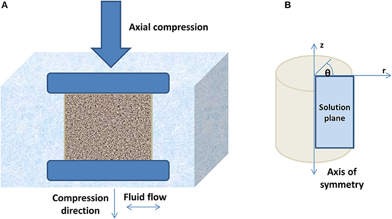
Figure 1. (A) A central cross-section through an unconfined cylinder of a poroelastic material subjected to a sustained uniaxial compression between two rigid, frictionless impermeable and parallel plates. (B) The relaxation problem is solved on the cylindrical polar coordinate system using an axisymmetric finite element modeling (FEM) simulation, on the indicated right half plane only. The solution that describes the behavior of the entire cylinder could be obtained by rotating the solution plane through θ, the angle around the axis of symmetry of the cylindrical sample. The direction of the axial compression is defined to be along the z-axis and the radial fluid flow along the r-axis.

For the purposes of modeling the strain-relaxation loading problem, it is assumed that an infinitesimal axial compressive stress is applied instantaneously on the upper surface of the sample and sustained thereafter:

$\begin{array}{ll}{\sigma }_{\mathrm{zz}}\left(t\right)=\{\begin{array}{c}0t<0\\ -{\sigma }_{0}t\ge 0\end{array}& (4)\end{array}$

where σ_zz is the magnitude of the stress applied in the axial direction.

Assuming that no shear forces exist on the compression plates (i.e., no friction between the sample and the plates), the radially averaged radial strain inside the sample, which is equal to the global radial strain defined by the radial displacement of the curved cylindrical surface at r = a, is given as [16]:

$\begin{array}{l}{\epsilon }_{\text{rr}}\left(a,t\right)=\left({\sigma }_0\right)[\frac{\nu }{E}+\frac{\left(1-{\nu }^2\right)\left(1-2\nu \right)}{E}\\ {\displaystyle \sum _{\text{n}=1}^{\infty }\frac{{4\text{e}}^{\frac{-{\alpha }_{\text{n}}^2{H}_{A}k{\eta }^{-1}t}{a^2}}}{\left\{9{\alpha }_{\text{n}}^2{\left(1-\nu \right)}^2-8\left(1+\nu \right)\left(1-2\nu \right)\right\}}}]& (5)\end{array}$

Furthermore, the axial strain history at r = a is given as follows [16]:

$\begin{array}{l}{\epsilon }_{\text{zz}}\left(t\right)\\ =-\frac{{\sigma }_0}{E}\left[1-{\displaystyle \sum _{\text{n}=1}^{\infty }\frac{(1-{\nu }^2)(1-2\nu ){4\text{e}}^{\frac{-{\alpha }_{\text{n}}^2{H}_{A}k{\eta }^{-1}t}{a^2}}}{\left\{9{\alpha }_{\text{n}}^2{\left(1-\nu \right)}^2-8(1+\nu )(1-2\nu )\right\}}}\right]& (6)\end{array}$

The evolution of the dilatation or volumetric strain, defined as the relative change in volume $\frac{\Delta V}{V}$ [22] within an element of a sample, is given as [16]:

$\begin{array}{l}{\epsilon }_{\text{v}}\left(r,t\right)\\ =-\frac{{\sigma }_0}{E}\left[\left(1-2\nu \right)-{\displaystyle \sum _{\text{n}=1}^{\infty }\frac{\left(1-2{\nu }^2\right)\left(1+\nu \right)\frac{{8\text{J}}_0\left({\alpha }_{\text{n}}r\right)}{a{J}_0({\alpha }_n)}{\text{e}}^{\frac{-{\alpha }_{\text{n}}^2{H}_{A}k{\eta }^{-1}t}{a^2}}}{\left\{9{\alpha }_{\text{n}}^2{\left(1-\nu \right)}^2-8\left(1+\nu \right)\left(1-2\nu \right)\right\}}}\right]& (7)\end{array}$

where α_n are the roots of the characteristic equation:

$\begin{array}{ll}{\text{J}}_0(\text{x})-\frac{4(1-2\text{v})}{3(1-\text{v})}\frac{{\text{J}}_1(\text{x})}{\text{x}}=0& (8)\end{array}$

where J₀ (x) and J₁(x) are the Bessel functions of the first kind of order 0 and 1, respectively, and ν is the Poisson's ratio.

For the purposes of modeling the stress-relaxation loading problem, an infinitesimal compressive axial strain is assumed to have been applied instantaneously on the upper surface of the sample and sustained thereafter:

$\begin{array}{ll}{\epsilon }_{\text{zz}}\left(t\right)=\{\begin{array}{cc}0& t<0\\ -{\epsilon }_0& t\ge 0\end{array}& (9)\end{array}$

where ε₀ is the magnitude of the strain applied in the axial direction.

For all times, the radially averaged radial strain inside the sample is given as [16]:

$\begin{array}{ll}{\epsilon }_{rr}(a,t)={\epsilon }_0\left[\nu +(1-2\nu )(1-\nu ){\displaystyle \sum _{\text{n}=1}^{\infty }}\frac{{\text{e}}^{\frac{{\beta }_n^2{H}_{A}k{\text{η}}^{-1}t}{a^2}}}{\left\{{\beta }_{\text{n}}^2{(1-\nu )}^2-(1-2\nu )\right\}}\right]& (10)\end{array}$

This equation for stress relaxation is equivalent to that for strain relaxation (Equation 5). The evolution of the radial strain field over radius and time is [8]:

$\begin{array}{ll}{\epsilon }_{rr}(r,t)={\epsilon }_0\left[\text{v}+{\displaystyle \sum _{\text{n}=1}^{\infty }}\frac{{\text{J}}_0({\beta }_{\text{n}})-\left(\frac{1-2\nu }{1-\nu }\right)\left\{\frac{{\text{J}}_0(r{\beta }_{\text{n}})}{a}-\frac{{\text{J}}_1\left(\frac{r{\beta }_{\text{n}}}{a}\right)}{\frac{r{\beta }_{\text{n}}}{a}}+\frac{{\text{J}}_1({\beta }_{\text{n}})}{{\beta }_{\text{n}}}\right\}}{\frac{1}{(1-\nu )}{\text{J}}_0({\beta }_{\text{n}})-{\beta }_{\text{n}}{\text{J}}_1({\beta }_{\text{n}})}{\text{e}}^{-\frac{{\beta }_{\text{n}}^2{H}_{A}k{\eta }^{-1}}{a^2}t}\right]& (11)\end{array}$

Finally, the radial and temporal variations of the dilatation or volumetric strain during stress relaxation are [8]:

$\begin{array}{ll}{\epsilon }_{\text{v}}(r,t)={\epsilon }_0\left[1-2\nu -{\displaystyle \sum _{\text{n}=1}^{\infty }}\frac{{2\text{J}}_0({\beta }_{\text{n}})-\left(\frac{1-2\nu }{1-\nu }\right)\left\{\frac{{\text{J}}_0({r\beta }_{\text{n}})}{a}+\frac{{2\text{J}}_1({\beta }_{\text{n}})}{{\beta }_{\text{n}}}\right\}}{\frac{1}{(1-\nu )}{\text{J}}_0({\beta }_{\text{n}}){-\beta }_{\text{n}}{\text{J}}_1({\beta }_{\text{n}})}{\text{e}}^{-\frac{{\beta }_{\text{n}}^2{H}_{A}k{\eta }^{-1}}{a^2}t}\right]& (12)\end{array}$

where β_n are the roots of the characteristic equation:

$\begin{array}{ll}{\text{J}}_1(x)-\frac{(1-\nu )}{(1-2\nu )}{x\text{J}}_0(x)=0& (13)\end{array}$

By setting t → ∞, the steady-state dilatation is equal to:

$\begin{array}{ll}{{\epsilon }_{\text{v}}(r,t)=\epsilon }_0\left[(1-2\nu )\right]& (14)\end{array}$

regardless of whether a stress relaxation or strain relaxation compression is used.

In reaching this steady state, the dilatation equation describes diffusion-like propagations of volumetric strain relaxation in a radial direction across the whole volume of a cylinder, beginning at the outer boundary and ending when it reaches the center of a sample. This propagation was chosen to be a qualitative and quantitative metric of comparison of the two loading configurations. Time-varying images showing this propagation of a volumetric strain relaxation were shown from the finite element simulations in Berry et al. [8] and confirmed experimentally in tissue mimicking poroelastic phantoms in Berry et al. [9]. In addition, the accuracy and precision of the poroelastic material characteristics, H_Ak and ν, recovered by fitting the predictions of the above equations to the results of the experiments simulated by FEM (see below), were used for further quantitative comparison of the utility of the two loading configurations.

Finite Element Modeling

A commercial FEM program, MARC Mentat^® (MSC Software Ltd., Frimley, UK), as used for poroelastic simulations by Fromageau et al. [12, 15], was employed to predict the response of an unconfined cylindrical sample to an externally applied stress relaxation or strain relaxation compression using a structural and diffusion-type simulation. The cylindrical geometry was used for the reasons provided at the beginning of the Section entitled The Poroelastic Sample Under Relaxation Compression. In both strain and stress-relaxation scenarios, the material of a sample was simulated to be a poroelastic fluid–solid mixture that obeys the consolidation and biphasic theories [16, 19]. The sample was compressed along its axis of symmetry between two frictionless, rigid, impermeable, flat, parallel surfaces while immersed in a fluid with a viscosity equal to that of water at room temperature. The axisymmetric relaxation problem was solved in cylindrical polar coordinates, for the right half of the z–r solution plane (Figure 1B).

The FEM mesh was composed of 1,000 elements (type 33 MARC Mentat^®) and 29,209 nodes, arranged in consecutive rows with a constant density throughout the homogenous cylindrical model. The height of the simulated cylinder was set equal to 30 mm and its radius equal to 25 mm, similar to that employed in the ultrasound strain imaging of poroelastic cylinders undergoing the stress-relaxation experiments of Berry et al. [9]. The poroelasticity of the model was satisfied by setting the porosity equal to 0.5 and the permeability of the simulated biphasic sample to the pore fluid equal to 6.4e-16 m². The permeability value was chosen to reflect the value expected in healthy soft tissue [13]. Other material properties are shown in Table 1. Fluid flow was prevented along the z-axis but allowed radially, conditions which allowed a good match to be achieved between the results from simulation and experiment in a previous study of poroelastic cylinders [8, 9]. The time step for sampling the temporal evolution of the strain field was 0.5 s.

TABLE 1

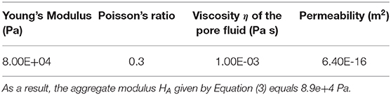
Table 1. The material properties specified for the simulated poroelastic sample.

Strain relaxation was simulated by loading the upper surface of a sample with a compressive axial stress of 4 kPa, corresponding to an axial force of 8 N uniformly distributed across the sample cross-section, allowing the upper surface to move while ensuring that the bottom plate was stationary.

Stress relaxation was simulated by moving the upper compressor plate along the z-axis, to apply a displacement to the upper surface of a sample with a magnitude equal to 3% of the height of a sample.

The axial stress or strain was sustained for 180 min. As frictionless boundaries had been assumed, the resulting axial and volumetric deformations of the sample were independent of the z-axis component of their location.

All strain components were simulated for both strain-relaxation and stress-relaxation experiments. Using the strain components, the volumetric strain was calculated so that the poroelastic sample behavior in strain relaxation could be compared with that in stress relaxation. Inserting the material properties (Table 1) into the strain equations of poroelasticity [Equations (5)–(7) and (10)–(12)] the deformation of the poroelastic sample was also analytically modeled during stress relaxation or strain relaxation for the same boundary conditions, time, and the applied compression as that employed in the FEM.

Estimation of Poroelastic Characteristics of a Material

The method previously employed by Berry et al. [8, 9], for estimating the poroelastic characteristics of the material of a cylinder under stress-relaxation loading, was applied again here, but also for strain-relaxation loading. By examining the poroelastic equations, it is straight forward to observe that not only do all equations share the same exponential mathematical form but also, importantly, their exponential decay is determined by the same time constant $\frac{{s_{\text{n}}}^2}{t_r}$, where s_n (α_n, β_n) are the eigenvalues of the characteristic equations (Equations 8 and 13) and t_r is the characteristic poroelastic relaxation time. This is the characteristic strain diffusion time of the porous matrix, determined as defined below by the square of the length of the maximum fluid path (which in this case is equal to the radius of a cylinder), the aggregate modulus H_A (Equation 3), the permeability k of the matrix, and the viscosity η of the pore fluid.

The parameterized form of the mathematical equations that describe the imaged strain in a poroelastic relaxation experiment may be written as follows:

$\begin{array}{ll}\text{strain }(r,t)={\text{P}}_{\text{i}}\left[A_i+{\displaystyle \sum _{\text{n}=1}^{\infty }}{B_i\text{e}}^{-\frac{{s_n}^2}{t_r}t}\right]& (15)\end{array}$

The constants of Equation (15) that are related to the volumetric strain ε_v in a strain relaxation compression experiment (Equation 7) are equal to:

$\begin{array}{l}{\mathit{P}}_1=-\frac{{\sigma }_0}{E}\\ A_1=(1-2\nu )\\ {\mathit{B}}_1=-\frac{\left(1-{2\nu }^2\right)(1+\nu )\frac{8J_0({\alpha }_{\text{n}}r)}{a{J}_0({\alpha }_{\text{n}})}}{\left\{9{{\alpha }_{\text{n}}^2(1-\nu )}^2-8(1+\nu )(1-2\nu )\right\}}\\ t_{\text{r}}=\frac{a^2}{H_{A}k{\eta }^{-1}}\end{array}$

and s_n = α_n, the roots of the characteristic equation (Equation 8).

On the other hand, the constants related to the volumetric strain ε_v in a stress relaxation compression experiment (Equation 12) are equal to:

$\begin{array}{l}{\mathit{P}}_2={\epsilon }_0\\ {\mathit{A}}_2=1-2\nu \\ {\mathit{B}}_2=-\frac{2{\text{J}}_0({\beta }_{\text{n}})-\left(\frac{1-2\nu }{1-\nu }\right)\left\{\frac{{\text{J}}_0(r{\beta }_n)}{a}+\frac{2{\text{J}}_1({\beta }_{\text{n}})}{{\beta }_{\text{n}}}\right\}}{\frac{1}{(1-\nu )}{\text{J}}_0({\beta }_{\text{n}})-{\beta }_{\text{n}}{\text{J}}_1({\beta }_{\text{n}})}\\ t_r=\frac{a^2}{H_{A}k{\eta }^{-1}}\end{array}$

and s_n = β_n, the roots of the characteristic equation (Equation 13).

For the cylindrical poroelastic phantom specified in Figure 1 and Table 1, the applied axial stress σ₀ or strain ε₀, the radius of the sample a, and the roots of the characteristic equations s_n are known. Thus, the parameters, determined by the poroelastic characteristics of the material from which the phantom is made, recovered by fitting the appropriate equation mentioned above to the strain data acquired during stress relaxation or strain-relaxation are:

$\begin{array}{l}{p}_1=v\\ p_2=p_{21}\ast p_{22}=H_A\ast k& (16)\end{array}$

There is only one equation in which the parameters p₂₁ and p₂₂ are employed for the relaxation time $t_r=\frac{a^2}{H_{A}k{\eta }^{-1}}$. Thus, it is impossible to separate the parameters p₂₁ and p₂₂ directly by model fitting without compromising the uniqueness of the solution.

The Levenberg–Marquardt (LM) algorithm that is available in the Matlab^® (Mathworks Inc., Natick, MA, USA) optimization toolbox was employed in this work to fit the above poroelastic equations to the FEM-predicted volumetric strain data. The goodness of fit was computed on 10 by 10 matrices of the simulated strain data produced by a forward analytical modeling using the poroelastic volumetric strain equations for strain relaxation (Equation 7) or stress relaxation (Equation 12). The flow chart (Figure 2) describes the LM algorithm steps.

FIGURE 2

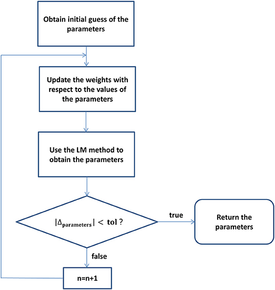
Figure 2. The flow chart describing the steps of the Levenberg–Marquardt (LM) optimization method.

A small percentage of random, uncorrelated noise with a flat probability density function (white noise) was added to the simulated strain data to mimic the random noise that exists in experimentally acquired data sets. Computationally, the noise was created by randomly varying each strain pixel within a range equal to ±3% of the respective strain value. The flat probability density function was chosen, instead of another function such as a Gaussian, to render the results unbiased with respect to the noise properties of any particular ultrasound acquisition system.

Starting from an arbitrary initial guess of the material properties, p₁ = [0.05 – 0.2], p₂ = [1 – 7] × 10⁻¹⁰ Pa m², the LM algorithm attempted to converge on the values that result in the best fit to the strain vs. time curves. The criteria used to assess data fitting were (a) the final value of the minimization cost function after an iteration had been stopped, and (b) the accuracy and precision of the estimated values of the material properties by comparing them with the predefined values (Table 1).

Results

Previously published studies in the area of experimental poroelasticity measurement using ultrasound have combined the mathematical models of poroelasticity with a finite element analysis to predict and validate the strain evolution inside a poroelastic cylinder subjected to a stress relaxation compression under unconfined boundary conditions [7, 8]. In this work, the analysis was extended to compare the results with those for an unconfined strain relaxation compression. The two types of compression induce distinct fluid-flow-related effects along the axial, radial, and circumferential axes.

In order to qualitatively and quantitatively compare the strain relaxation with the stress-relaxation (of a poroelastic material subjected to an unconfined compression), an objective metric is necessary. For this purpose, the fluid-induced internal strain behavior was simulated for both types of relaxation and the results are shown in the figures. The diffusion-like propagation of the volumetric strain across the whole volume of the cylinder, and the accuracy, precision, and appearances of the images of the poroelastic material characteristics, H_Ak and ν, recovered by fitting the predicted time-varying strain to the measured time-varying strain, were used as the qualitative and quantitative metrics of comparison of the two loading configurations.

Comparison of Two Types of Poroelastic Relaxation Behavior Using Finite Element Analysis and Analytical Modeling

The strain across each polar coordinate was modeled by using a finite element analysis. The behavior of the deformation of a poroelastic cylinder was determined by subjecting it to an axial stress and an equivalent axial strain sustained for 3 h. Figures 3–6 show the evolution of the axial, radial, circumferential, and volumetric strains, respectively, at the axial center and across the radius of a poroelastic sample subjected to a constant axial stress (strain relaxation, left figure) and a constant axial strain (stress relaxation, right figure), determined by using a finite element analysis. The volumetric strain is the sum of the axial strain, the radial strain, and the circumferential strain.

FIGURE 3

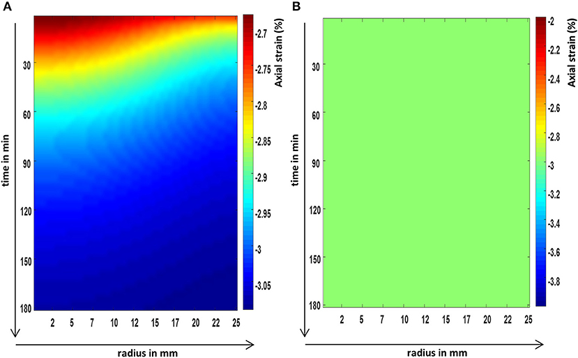
Figure 3. The FEM predictions of the axial strain evolution over time, at the axial center, and across the radius of a cylindrical poroelastic sample subjected to a constant axial stress (A) and an equivalent constant axial strain (B).

FIGURE 4

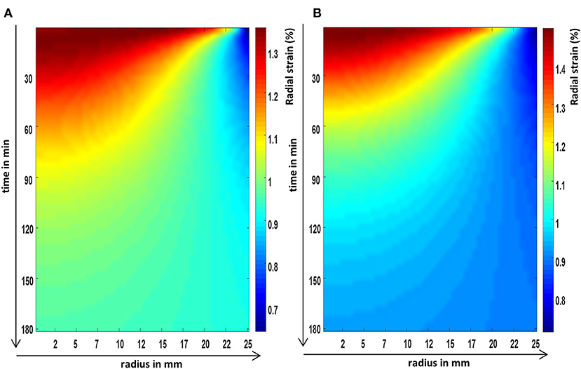
Figure 4. The FEM predictions of the radial strain evolution over time, at the axial center, and across the radius of a cylindrical poroelastic sample subjected to a constant axial stress (A) and an equivalent constant axial strain (B).

FIGURE 5

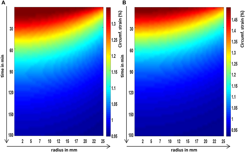
Figure 5. The FEM predictions of the circumferential strain evolution over time, at the axial center, and across the radius of a cylindrical poroelastic sample subjected to a constant axial stress (A) and an equivalent constant axial strain (B).

FIGURE 6

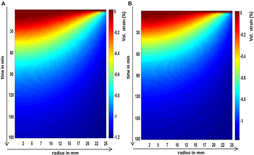
Figure 6. The FEM predictions of the evolution of the volumetric strain or dilatation over time, at the axial center, and across the radius of a cylindrical poroelastic sample subjected to a constant axial stress (A) and an equivalent constant axial strain (B).

In Figures 7 and 8, for strain relaxation and stress relaxation, respectively, the FEM predictions (plotted symbols) and the analytical predictions (solid lines) of the time dependence of the volumetric strain inside the simulated biphasic cylinder are plotted throughout the radial extent of the phantom. The boundary conditions were the same for the FEM and the analytical calculations. Specifically, Figure 7 shows the spatial and temporal dependence of the volumetric strain inside a phantom in a strain relaxation compression. Figure 8 displays the volumetric strain behavior of the same phantom during stress relaxation.

FIGURE 7

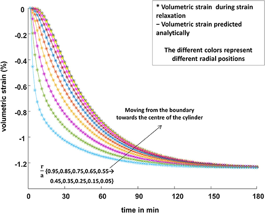
Figure 7. The FEM predictions of the spatially varying volumetric strain (“^*” symbols) inside a cylindrical poroelastic sample subjected to a constant compressive axial force, undergoing strain relaxation, are plotted along with the analytical predictions (Equation 7; solid lines). The volumetric strain decreases more rapidly for large values of the radial position r, where the pore fluid first leaves the sample, than for positions closer to the center of the cylinder, where the fluid contained in the pores is the last to leave its original location. The different colors represent different radial positions, r/a: cyan 0.95, lime 0.85, purple 0.75, yellow 0.65, orange 0.55, blue 0.45, brown 0.35, magenta 0.25, yellow 0.15, and olive 0.05.

FIGURE 8

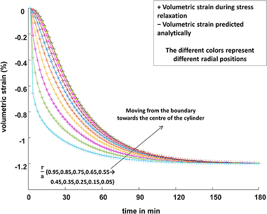
Figure 8. The FEM predictions of the spatially varying volumetric strain (“+” symbols) inside a cylindrical poroelastic sample subjected to a constant compressive axial strain, undergoing stress relaxation, are plotted along with the analytical predictions (Equation 12; solid lines). Similar to the strain-relaxation case in Figure 7, the volumetric strain decreases most quickly at the larger values of the radial position r where the fluid path out of the sample is shorter. The different colors represent different radial positions, r/a: cyan 0.95, lime 0.85, purple 0.75, yellow 0.65, orange 0.55, blue 0.45, brown 0.35, magenta 0.25, yellow 0.15, and olive 0.05.

Figure 9 compares the volumetric strain behavior, averaged across the whole solution plane, computed by using an FEM and analytically, for the two different types of axial compression.

FIGURE 9

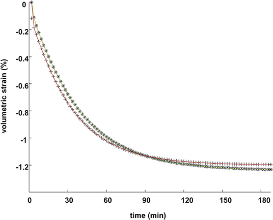
Figure 9. The FEM predictions (plotted symbols) of the volumetric strain behavior over time, spatially averaged across all radial positions, compared with the analytical predictions of Equations (7) and (12) (solid lines), in the strain relaxation (olive lines and stars) and the stress relaxation (brown lines and crosses) compressions of a sample.

Equivalence of Strain Relaxation and Stress Relaxation for Using an Inverse Method to Determine the Poroelastic Material Properties

Table 2 shows the values of the extracted material properties averaged over the whole region of interest inside a poroelastic cylinder undergoing strain relaxation or stress relaxation. The poroelastic properties (p1 and p2) were estimated by applying an LM inverse method to the strain-relaxation and stress-relaxation strain data, produced directly from the equations of poroelasticity, for 10 realizations of the algorithm, employing different initial parameters and white noise each time. The estimated values and the true parameter values that were predefined for the simulated poroelastic phantom may be observed in Table 1. Table 2 shows the values for the cost function that is a goodness-of-fit parameter.

TABLE 2

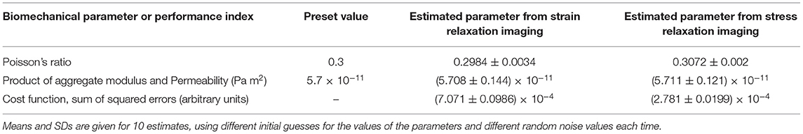
Table 2. The performance of the inverse method was tested by using the strain data generated from FEM simulation of a poroelastic phantom undergoing a stress or strain relaxation compression, with predefined biomechanical properties.

Figure 10 displays, for both the strain and the stress relaxation compressions, the material property and the cost function images that were derived by applying an LM inverse method to fit the analytically predicted time-varying volumetric strain to the FEM-measured time-varying volumetric strain at each of the 10 × 10 pixel locations inside a poroelastic cylinder.

FIGURE 10

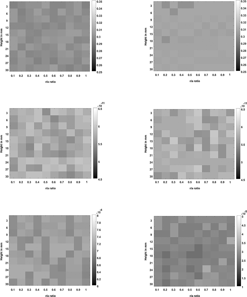
Figure 10. The images of the poroelastic model parameters such as the Poisson's ratio (top row) and the product of aggregate modulus and permeability (middle row), and the images of the cost function values per pixel (bottom row). The left column shows the images that were recovered from a simulated poroelastic phantom subjected to a strain relaxation compression (an applied force of −8 N), and the right column shows the images that were recovered from a simulated poroelastic phantom subjected to a stress relaxation compression (applied strain of −3%). The grayscale bars were arbitrarily scaled to allow comparisons, with maxima and minima chosen to include the maximum and minimum pixel values within each image.

Discussion

In this work, the fluid-induced strain within a poroelastic phantom in a typical in vitro experimental relaxation scenario was predicted by using both analytical and finite element methodologies. Furthermore, biomechanical material property images were created by recovering the poroelastic parameters from the simulated strain data using an LM inverse method. In all simulations, the experimental design, biomechanical properties, and geometry of a sample were identical.

The central question that was being asked was, does a strain relaxation compression experiment provide the same quantitative and qualitative information about the poroelastic nature, behavior, and properties of the studied sample as a stress-relaxation experiment?

In order to compare the two loading configurations, both relaxation experiments were simulated identically, with the only difference being that in the strain relaxation, a constant axial force was applied and in the stress relaxation an axial strain was held constant. All strain components were simulated for both strain relaxation and stress relaxation. The volumetric strain was selected as an unbiased metric of comparison of the poroelastic sample behavior in the two different types of relaxation.

There was a good agreement between the phantom dilatations obtained using the strain relaxation and stress relaxation, and this result was independent of the duration of the relaxation (Figure 6).

The pixel-by-pixel dilatation data obtained by the FEM, from the boundary to the center of the simulated phantom, were in excellent agreement with the analytical predictions of the equations of poroelasticity for the same biomechanical properties and boundary conditions as simulated by FEM (Figures 7, 8).

The relative ability to use stress relaxation and strain relaxation experiments to recover the poroelastic properties of the simulated phantom was assessed by fitting the volumetric strain produced directly from the equations of poroelasticity to the “measured” data generated by the FEM simulation. The LM inverse method successfully converged close to the correct values of the material properties for both hypothetical strain and stress-relaxation experiments, independent of the poor initial guess of the material properties and the random noise added in the simulated strain data. The LM algorithm located the minima of the cost functions and converged precisely and accurately to the parameter p₁ (Poisson's ratio) and the parameter p₂ (product of the aggregate modulus and permeability), with respective mean values and SDs displayed in Table 1, just as well for the strain relaxation loading as it did for the stress relaxation loading. Images of the local values of the Poisson's ratio and the product of the aggregate modulus and permeability were created, again demonstrating equal capability and performance for the strain relaxation loading as for stress relaxation loading. For the simulation of homogeneous media, the Poisson's ratio and aggregate modulus maps in Figure 10 illustrate a desirable absence of spatial bias in the solution to which the inversion method converged. They also indicate the level of variation to be expected, for the noise level employed in this simulation. Finally, they illustrate the capability to produce the quantitative images of these novel biomechanical properties, which for biological tissues should show spatial variation that may be expected to highlight differences for different tissues and spatially localized pathology.

However, it should be noted that the determination of the characteristics of a poroelastic material by fitting a time-varying strain at a point to the analytical predictions is applicable only to the conditions to which the analytical theory applies, i.e., in this case to the cylindrical samples of homogeneous materials where the biomechanical properties are not varying significantly over time and space. The implication of this assumption is that to apply this method in the laboratory, homogenous cylindrical phantoms of controlled mechanical properties need to be made and tested under strictly monitored experimental conditions. Moreover, to extend the application of the method in vivo, the inverse method should be further developed to account for tissue inhomogeneities, non-linearity, anisotropy, and viscoelasticity of the solid matrix, a variation in tissue permeability due to the different types of fluid flow and widely varying (i.e., non-cylindrical) boundary conditions, including the varying levels of confinement provided by surrounding tissues. Also not considered is the in vivo feasibility of applying and tracking tissue deformations for the long periods that may be necessary. Nevertheless, the positive results of previous in vivo studies involving various types of loading and strain measurement [10, 11, 14], provide substantial encouragement that our findings concerning the strain-relaxation loading should be applicable for poroelastography in vivo.

The noise model employed in the simulation, which was spatially uncorrelated and has a uniformly distributed probability density function, may not reflect the correlations and distribution of noise in ultrasonically generated estimates of strain, which may also be anisotropic showing the largest variance in the lateral direction. A further limitation is that only a single noise level was simulated rather than a range of signal-to-noise ratios. However, these limitations should not impact negatively on the main finding that, for quantitative poroelastography, strain relaxation (which may have practical advantages as described below) represents a viable alternative loading condition to stress relaxation. In fact, the use of a more accurate noise model with a greater strain estimation variance in the lateral direction is likely to have further emphasized the benefits of strain relaxation, which can take advantage of a greater precision with which axial strain can be measured. Nevertheless, further work would be helpful to understand whether there are differences between the two approaches in terms of sensitivity to noise.

By studying the strain inside a cylindrical phantom, it has been found from these simulations that either a constant axial stress or strain may be used for quantitative poroelastography because they generate a similar and predictable temporal and spatial variation of internal strain when applied to the same phantom. Although a cylindrical geometry is unlikely to occur naturally in the body (apart from, perhaps, intervertebral discs), it is sufficient here to allow a qualitative and quantitative comparison of the experiments of strain relaxation and stress relaxation. If an inversion method for recovering the quantitative values and the images of the characteristics of a poroelastic material was to be applied in vivo, however, sample geometries other than cylindrical geometries may need to be modeled. For such purposes, analytical modeling is likely to be too complex and a more feasible approach may be to extract parameters from the simulations that best fit the ultrasound-measured spatially varying and time-varying strain. The input data for such simulations, regarding the organ (such as breast, liver, and brain) boundary shape, for example, could be obtained from 3D medical images such as those obtained using MRI, x-ray CT, or ultrasound. In such future work, however, it would also be necessary to extend the modeling to predict the behavior under conditions of localized compression (indentation) of large organs [15].

The reader should note though that the creep (strain relaxation) poroelastic results simulated herein may not be easily replicated experimentally using a rigid compressor because the compressor may not permit the radially varying axial strain shown in Figure 3A in all axial locations. Sridhar et al. [23] and Qiu et al. [14] performed creep experiments using a rigid compressor for the purposes of studying a viscoelastic behavior and did not report behavior such as that shown in Figure 3A, although they were not specifically looking for such effects. For the optimal laboratory replication of the strain-relaxation results shown here, a much more sophisticated non-rigid way of applying the constant axial stress would be ideal, possibly by using an indenter array or a fluid compressor. Alternatively, a rigid compressor may yield useful results for some axial locations, or a more complete understanding of the axial variation of the time-varying and radially varying strain may allow more general use of a rigid compressor.

The stress relaxation experiments are relatively easily implemented in a laboratory using a conventional rigid compressor to sustain an axial strain on the top surface of a poroelastic sample. Indeed, Berry [24], using an FEM and experiments in vitro, reported a poroelastic strain response during stress relaxation that was like that shown in Figures 3B–6B. Strain relaxation, on the other hand, could be advantageous if one considers potential clinical imaging setups.

If 3D ultrasound methods for accurately estimating all three components of strain and their temporal evolution were available, the dilatation of the poroelastic sample could be imaged during the relaxation [12]. This would be an ideal echo imaging system for poroelastography because it could quantify the change in the volume of the poroelastic sample, which would be equal to the fluid that has flowed out of the matrix during relaxation. If only one accurately estimated component of strain is available (i.e., along the ultrasound beam axis), which is typically the case for two-dimensional (2D) or 3D ultrasound imaging, then a strain-relaxation (creep) methodology may have advantages compared with a stress-relaxation method, since it exhibits a time-varying axial strain whereas for stress relaxation it does not (compare Equation 6 with Equation 9, and Figures 3A,B). Importantly for clinical applications, if axial strain alone could be employed, it would allow the ultrasound probe to be used for both compression and imaging, avoiding the errors and difficulty of lateral and elevational strain estimation.

It was shown in the FEM images (Figures 3–5) that all poroelastic strain components vary spatially and all components contribute to the local dilatation information (Figure 6A) during strain (creep) relaxation. In a stress relaxation case, as axial strain is fixed, only the radial and circumferential strain components (Figures 4B and 5B) contribute to the local dilatation information (Figure 6B). Thus, the mathematical formulation of each compression problem should be considered before selecting the most appropriate experimental design.

Overall, an important potential advantage of the creep methodology is the possibility to derive useful information related to the biomechanical nature of a sample by imaging the time evolution of the axial strain only, avoiding the technical difficulties and errors associated with the volumetric or even axial-to-lateral strain ratio calculation.

Conclusions

Based on both the FEM and analytical results, it is evident that the diffusion-like strain behavior during the relaxation of an unconfined poroelastic sample under compressive loading is determined entirely by its elastic constants (aggregate modulus, Poisson's ratio, and Young's modulus), and by the permeability of its matrix to the pore fluid and the radial flow path length. Regardless of whether the type of sustained compression employed eliceted strain or stress relaxation, the simulated relaxations of a poroelastic sample with interstitial permeability and Poisson's ratio similar to a healthy tissue, resulted in a similar magnitude of volumetric strain at equilibrium. Similar spatially varying and time-varying dilatations of a poroelastic cylinder were observed in a relaxation compression, independent of the type of loading, as long as other boundary conditions remained unchanged. Therefore, both unconfined compression methodologies permit the study of the poroelastic deformation of a sample. Most importantly, either of the unconfined compression configurations could be applied experimentally to obtain the qualitative and quantitative information related to the biomechanical nature of a chosen poroelastic sample. For eventual clinical application of the method for recovering the quantitative poroelastic parameters and images, it will be necessary to consider sample geometries other than the cylindrical geometry with, for example, an inversion by fitting the predictions of simulations to the ultrasound measurements of the spatially varying and time-varying strain.

This work shows that both unconfined compression relaxation methodologies could in principle be applicable in vitro and in vivo and strain relaxation provides several potential advantages due to the fact that the strain variation could be imaged by axial displacement tracking with the ultrasound beam aligned along the axis of compression, which bypasses the need for the estimation of lateral strain and elevational strain and significantly simplies the setup for in vivo scanning and compression.

Data Availability Statement

The original contributions presented in the study are included in the article. Further inquiries can be directed to the corresponding authors.

Author Contributions

MT performed the computations and analyzed the data under the supervision of JF, JB, and NdS. JF and JB assisted with the analysis and JF helped to carry out the FEM simulations. MT wrote the manuscript in consultation with JF, NdS, and JB. All authors contributed to the article and approved the submitted version.

Funding

This research was funded by the Cancer Research UK Cancer Imaging Center at the Institute of Cancer Research (Grant C1060/A16464). We also acknowledge the NIHR support of the Biomedical Research Center (BRC) at the Institute of Cancer Research and Royal Marden Hospital.

Conflict of Interest

The authors declare that the research was conducted in the absence of any commercial or financial relationships that could be construed as a potential conflict of interest.

References

1. Levick JR. An Introduction to Cardiovascular Physiology, 4th ed. London: Arnold Publishers (2003).

Google Scholar

2. Melody AS, Fleury ME. Interstitial flow and its effects in soft tissues. Annu Rev Biomed Eng. (2007) 9:229–56. doi: 10.1146/annurev.bioeng.9.060906.151850

PubMed Abstract | CrossRef Full Text | Google Scholar

3. Duck FA. Physical Properties of Tissue: A Comprehensive Reference Book. London: Academic Press Ltd. (1990). doi: 10.1016/B978-0-12-222800-1.50010-3

CrossRef Full Text | Google Scholar

4. Fung Y, Cowin S. Biomechanics: mechanical properties of living tissues. J Appl Mech. (1994) 61:1007. doi: 10.1115/1.2901550

CrossRef Full Text | Google Scholar

5. Bates DO, Levick JR, Mortimer PS. Quantification of rate and depth of pitting in human edema using an electronic tonometer. Lymphology. (1994) 27:159–72.

PubMed Abstract | Google Scholar

6. Bamber JC, Cosgrove DO, Dietrich CF, Fromageau J, Bojunga J, Calliada F, et al. EFSUMB Guidelines and recommendations on the clinical use of ultrasound elastography. Part 1: basic principles and technology. Ultraschall Med. (2013) 34:169–84. doi: 10.1055/s-0033-1335205

PubMed Abstract | CrossRef Full Text | Google Scholar

7. Konofagou E, Harrigan TP, Ophir J, Krouskop TA. Poroelastography: Imaging the poroelastic properties oftissues. Ultrasound Med Biol. (2001) 27:1387–97. doi: 10.1016/S0301-5629(01)00433-1

CrossRef Full Text | Google Scholar

8. Berry GP, Bamber JC, Armstrong CG, Miller NR, Barbone PE. Towards an acoustic model-based poroelastic imaging method: I. theoretical foundation. Ultrasound Med Biol. (2006) 32:547–67. doi: 10.1016/j.ultrasmedbio.2006.01.003

PubMed Abstract | CrossRef Full Text | Google Scholar

9. Berry GP, Bamber JC, Miller NR, Barbone PE, Bush NL, Armstrong CG. Towards an acoustic model-based poroelastic imaging method: II. experimental investigation. Ultrasound Med Biol. (2006) 32:1869–85. doi: 10.1016/j.ultrasmedbio.2006.07.013

PubMed Abstract | CrossRef Full Text | Google Scholar

10. Berry GP, Bamber JC, Mortimer PS, Bush NL, Miller NR, Barbone PE. The Spatio-temporal strain response of oedematous and nonoedematous tissue to sustained compression in vivo. Ultrasound Med Biol. (2008) 34:617–29. doi: 10.1016/j.ultrasmedbio.2007.10.007

PubMed Abstract | CrossRef Full Text | Google Scholar

11. Righetti R, Garra BS, Mobbs LM, Kraemer-Chant CM, Ophir J, Krouskop TA. The feasibility of using poroelastographic techniques for distinguishing between normal and lymphedematous tissues in vivo. Ultrasound Med Biol. (2007) 52:6525–41.

PubMed Abstract | Google Scholar

12. Fromageau J, Bush N, Bamber J. Reliable estimation of permeability from the 4D strain distribution in poroelastic tissues. In: Proceedings of the IEEE Ultrasonics Symposium, Dresden, Oct. 7-10. Piscataway, NJ: IEEE (2012). p. 2529–32. doi: 10.1109/ULTSYM.2012.0633

CrossRef Full Text | Google Scholar

13. Leiderman R, Barbone PE, Oberai AA, Bamber JC. Coupling between elastic strain and interstitial fluid flow: ramifications for poroelastic imaging. Ultrasound Med Biol. (2006) 51:6291–313. doi: 10.1088/0031-9155/51/24/002

PubMed Abstract | CrossRef Full Text | Google Scholar

14. Qiu Y, Sridhar M, Tsou JK, Lindfors KK, Insana MF. Ultrasonic viscoelasticity imaging of nonpalpable breast tumors: preliminary results. Acad Radiol. (2008) 15:1526–33.

PubMed Abstract | Google Scholar

15. Fromageau J, Berry G, Bamber J. The spatio-temporal strain distribution in inhomogeneous poro-elastic phantoms. In: Proceedings of the IEEE Ultrasonics Symposium, Rome, Sep. 20-23 2009, Yuhas MP, editor. Piscataway, NJ: IEEE (2009). p. 2437–40. doi: 10.1109/ULTSYM.2009.5441859

CrossRef Full Text | Google Scholar

16. Armstrong C, Lai W, Mow V. An analysis of the unconfined compression of articular cartilage. J Biomech Eng. (1984) 106:165. doi: 10.1115/1.3138475

PubMed Abstract | CrossRef Full Text | Google Scholar

17. McCrum NG, Buckly CP, Bucknall CB. Principles of Polymer Engineering 2nd ed. Oxford: OUP (1997).

Google Scholar

18. Lakes RS. Viscoelastic Solids. Boca Raton, FL: CRC Press (1998).

Google Scholar

19. Biot MA. General theory of three-dimensional consolidation. J Appl Phys. (1941) 12:155–4. doi: 10.1063/1.1712886

CrossRef Full Text | Google Scholar

20. Theoddorou M. Quantitative Ultrasound Permelastography for Tissue Characterization. PhD thesis, London: University of London (2017).

21. Barbone PE, Oberai AA, Bamber JC, Berry GP, Dord J.-F, Ferreira ER, et al. Nonlinear and poroelastic biomechanical imaging: elastography beyond Young's modulus. Ch.15, In: Neu CP, Genin GM, editors. Handbook of Imaging in Biological Mechanics. Boca Raton, FL: CRC Press (2015). p. 199–215.

Google Scholar

22. Brady BHG, Brown ET. Rock Mechanics for Underground Mining. Melbourne, VIC: Allen and Unwin Ltd. (1985).

Google Scholar

23. Sridhar M, Liu J, Insana MF. Elasticity imaging of polymeric media. J Biomech Eng. (2007) 129:259–72. doi: 10.1115/1.2540804

CrossRef Full Text | Google Scholar

24. Berry GP. Acoustic Poroelasticity Imaging of Biological Tissues. PhD thesis, University of London, London, United Kingdom (2006).