Shear Wave Elastography Based on Noise Correlation and Time Reversal

Shear wave elastography (SWE) relies on the generation and tracking of coherent shear waves to image the tissue's shear elasticity. Recent technological developments have allowed SWE to be implemented in commercial ultrasound and magnetic resonance imaging systems, quickly becoming a new imaging modality in medicine and biology. However, coherent shear wave tracking sets a limitation to SWE because it either requires ultrafast frame rates (of up to 20 kHz), or alternatively, a phase-lock synchronization between shear wave-source and imaging device. Moreover, there are many applications where coherent shear wave tracking is not possible because scattered waves from tissue’s inhomogeneities, waves coming from muscular activity, heart beating or external vibrations interfere with the coherent shear wave. To overcome these limitations, several authors developed an alternative approach to extract the shear elasticity of tissues from a complex elastic wavefield. To control the wavefield, this approach relies on the analogy between time reversal and seismic noise cross-correlation. By cross-correlating the elastic field at different positions, which can be interpreted as a time reversal experiment performed in the computer, shear waves are virtually focused on any point of the imaging plane. Then, different independent methods can be used to image the shear elasticity, for example, tracking the coherent shear wave as it focuses, measuring the focus size or simply evaluating the amplitude at the focusing point. The main advantage of this approach is its compatibility with low imaging rates modalities, which has led to innovative developments and new challenges in the field of multi-modality elastography. The goal of this short review is to cover the major developments in wave-physics involving shear elasticity imaging using a complex elastic wavefield and its latest applications including slow imaging rate modalities and passive shear elasticity imaging based on physiological noise correlation.

1 Introduction

The goal of Shear Wave Elastography (SWE) is to measure the tissue’s shear elasticity μ (i.e. elasticity). To this end, SWE relies on shear wave propagation inside soft tissues, since under the assumption of a purely elastic isotropic medium, the shear wave speed $c_s$ is directly linked to μ through the relation $\mu =\rho .c_s^2$ (ρ being the tissue’s density). The standard sequence in many SWE modalities is the following: first, shear waves are generated by carefully applying an external controlled shear wave source (e.g., mechanical actuator or ultrasound radiation force). Then, the induced displacements are imaged, usually by using ultrasound or a magnetic resonance imaging (MRI) system. In ultrasound based SWE ultrafast frame rates (i.e. between 1 to 20 kHz) are required to track the shear wave propagation. Alternatively, for low frame rates imaging modalities, a phase-lock synchronization between acquisition and shear wave source is needed (e.g., in magnetic resonance elastography). Finally, the tissue’s shear elasticity is deducted from the measured displacement field by estimating the shear wave speed, or alternatively, the shear wavelength (i.e., if the shear wave excitation frequency is known). Recent technological developments have allowed SWE to be implemented in commercial ultrasound and MRI systems, quickly becoming a new imaging modality in medicine and biology [1–3].

In SWE, the shear wave speed is usually estimated from the coherent or ballistic shear wave propagation. However, there are many applications where coherent shear wave tracking is not possible due to the interference of scattered waves coming from tissue boundaries and internal inhomogeneities. Moreover, additional waves generated by muscular activity, heart beating or other sources of vibrations may interfere with the coherent shear wave resulting in a complex elastic wavefield. Directional filtering has been proposed to solve this issue [4, 5]. However, other researchers focused in developing alternative approaches to measure μ (or equivalently $c_s$) from a complex elastic wavefield [6–18]. For example, in the TREMR technique (Table-Resonance Elastography with MR), the elastic field created by the vibrations of the patient table of a MRI system was used to image the elasticity of a tissue phantom and the brain [7]. Moreover, several authors have chosen to take advantage of the complex elastic wavefield naturally present in the human body due to pulsatility, heart beating and muscular activity to conduct an elastography experiment [8–11, 13, 14, 19–21]. Due to the absence of any external shear wave source this approach is usually termed as passive elastography.

Recently, inspired by seismic noise correlation [22, 23] and time reversal [24] a novel method [12, 25, 26] to extract the shear elasticity of tissue from a complex elastic field was developed. The first step is to record the complex wavefield generated by random internal or external sources. Then, by cross-correlating the elastic field at different positions, which can be interpreted as a time reversal experiment in the computer [27], shear waves are virtually focused on any point of the imaging plane. From the computed time reversal field there are different independent approaches to image the shear elasticity [12–15, 18], for example, tracking the coherent shear wave as it focus; measuring the focus size which is directly linked to the shear wavelength (${\lambda }_s$) and hence to the shear wave velocity; or evaluating the vibration amplitude at the focusing point, since for a given frequency, the vibration amplitude is larger in a soft tissue than in a hard one. Because this method takes advantage of a complex elastic wavefield it has found important applications in passive elastography [13, 14].

The pioneering work in this field was done at the Laboratorio de Acústica Ultrasonora (LAU) in Montevideo, Uruguay in collaboration with Stefan Catheline, who was at the LAU for a 2 year mission. The work of Catheline et al. [25] presented the observation of a time reversal experiment using shear waves in a tissue-mimicking phantom for the first time. In [25] it was shown that, contrary to the scalar field case (e.g., in fluids), for an elastic field in the bulk of a soft tissue, the focus is no more isotropic. Instead, it has an ellipse-like shape leading to a direction dependent Rayleigh criterion. Then, Benech et al. [12] established numerically that the focus width at −6 dB was approximately equal to one shear wavelength. This approach was termed the focus size (or width) method and was used to measure the elasticity of a tissue mimicking phantom. This method was shown to be independent of the source kind, shape, and time excitation function. This robustness regarding the shear wave source allowed envisioning its application to passive elastography. Alternatively, in [12], the phantom’s elasticity was measured by tracking the phase of the coherent shear wave as it focused back to the source (i.e. the phase method). Both methods (phase and focus size), were also used by Brum et al. [26] to measure the elasticity of a tissue mimicking phantom and cheese using surface waves. Finally, the feasibility to conduct 2D elasticity imaging in vivo using passive elastography was demonstrated by Gallot et al. [13] in the human liver and belly muscle. To image the shear wave speed they used an ultrafast ultrasound scanner along with the phase and focus size methods. The main advantage of the focus size method is its compatibility with low imaging rates modalities. This was first shown in [12] and then used in [13] to conduct a shear wavelength tomography of a two-layered tissue-mimicking phantom. In Catheline et al. [14] it was further demonstrated that the loss of time and/or spatial coherence of the recorded wavefield is not an obstacle for a wavelength tomography, which led to new passive elastography experiments using optical coherence tomography (OCT) [21] and MRI [20]. Finally, in [15] an analytical expression that allowed converting the wavelength tomography into shear elasticity was derived. The compatibility with low imaging rates modalities has led to innovative developments and new challenges in the field of multi-modality elastography. Particularly, it has boost the concept of passive elastography to new applications involving ultrafast and ultraslow imaging modalities like ultrasound, optical methods (digital holography or OCT) and MRI.

In this context, the goal of this short review is to cover the major developments in wave-physics involving elasticity imaging using time reversal and noise correlation of shear waves together with its latest applications. These include time reversal physics and near field effects of shear waves in soft tissues [15, 28, 29], passive brain elasticity imaging using MRI [20], cornea elasticity imaging using OCT [21], thyroid [14] and breast [18] elasticity imaging using low frame rate ultrasound scanners, liver elasticity imaging [13, 30], passive muscle elasticity assessment [11, 19] and most recently cellular elasticity imaging [31].

2 Time Reversal and Noise Correlation of Shear Waves

Time reversal was first proposed by Mathias Fink [24] and is based on the time-reversal invariance of the wave equation in a lossless medium. Time-reversal focusing is a two-step process. In a first step, the direct wave scene is recorded: the impulse response of a point source placed in $\overrightarrow{r_0}$ is measured by a set of receivers forming a closed cavity around $\overrightarrow{r_0}$. In a second step, the recorded wavefield is time reversed and sent into the medium through the same position where it was received. As a consequence of the $t\to -t$ invariance of the wave equation in a lossless medium, the wave will travel the same original path but in opposite direction to finally focus at the original source position $\overrightarrow{r_0}$ and then diverges. Due to the impulsive character of the source, the time reversal field ${\psi }^{TR}\left(\overrightarrow{r_0},\overrightarrow{r},t\right)$ around $\overrightarrow{r_0}$ can be written as [32]:

${\psi }^{TR}\left(\overrightarrow{r_0},\overrightarrow{r},t\right)=G\left(\overrightarrow{r_0},\overrightarrow{r},-t\right)-G\left(\overrightarrow{r_0},\overrightarrow{r},t\right)(1)$

where $G\left(\overrightarrow{r_0},\overrightarrow{r},t\right)$ is the Greeen’s function between $\overrightarrow{r_0}$ and $\overrightarrow{r}$. Equation 1 clearly reflects the focusing process: the causal Green’s function $G\left(\overrightarrow{r_0},\overrightarrow{r},t\right)$ corresponds to a diverging wave from $\overrightarrow{r_0}$ while the acausal Green’s function $G\left(\overrightarrow{r_0},\overrightarrow{r},-t\right)$ corresponds to a converging wave toward $\overrightarrow{r_0}$. The maximum amplitude is found to be at $\overrightarrow{r_0}$ (focusing point) at time $t=0$ (focusing time).

In practice, an ideal time-reversal cavity as described above is not necessary and can be replaced by a time-reversal mirror using reverberation and/or a multiple scattering medium [33]. For elastography applications one can take advantage of multiple sources, reverberation and diffusion to conduct a time reversal experiment. Specifically, the step where the time reversed field is sent back into the medium (i.e., the second step in a time reversal experiment) is replaced by a virtual time-reversal experiment based on spatial reciprocity and cross-correlation of the wavefield [12].

Usually the imaging systems used in elastography (e.g., ultrasound, OCT or MRI) allow recording at least one component of the elastic wavefield within a given region of interest (ROI). Let this component be $\psi \left(\overrightarrow{r},t\right)$. The correlation field at a given position $\overrightarrow{r_0}$ is computed by cross-correlating the field $\psi \left(\overrightarrow{r_0},t\right)$ with the field $\psi \left(\overrightarrow{r},t\right)$ acquired at all other positions $\overrightarrow{r}$ within the ROI.

$C\left(\overrightarrow{r_0},\overrightarrow{r},t\right)=\psi \left(\overrightarrow{r_0},-t\right)\otimes \psi \left(\overrightarrow{r},t\right)(2)$

If the field is diffuse, Eq. 2 allows the retrieval of the Green’s function [34]:

$\frac{\partial }{\partial t}C\left(\overrightarrow{r_0},\overrightarrow{r},t\right)\propto G\left(\overrightarrow{r_0},\overrightarrow{r},-t\right)-G\left(\overrightarrow{r_0},\overrightarrow{r},t\right)(3)$

The analogy between time reversal and cross-correlation follows directly from comparing Eqs. 1, 3: the time derivative of the correlation field is proportional to the time-reversal field. The proportionality constant in Eq. 3 will depend on the propagation equation, medium and source properties, propagation regime, etc. For instance, in the case of a visco-elastic medium with homogeneously distributed white noise sources Gouedard et al. derived Eq. 3 with the factor $4a/{\sigma }^2$ on the left hand side, with a being the attenuation and σ the average source spectrum [35]. Moreover, if the displacement field has a finite bandwidth (as in most experiments), the correlation and its time derivative only differ in a constant phase change [36] and the correlation field may be directly interpreted as the time reversal field. Formally, the relation between cross-correlation and time-reversal can be expressed by a representation theorem of the correlation type [37]. Consider a lossless elastic medium with volume V and bounding surface S. Let $G_{mn}\left(\overrightarrow{r_0},\overrightarrow{r}\right)$ represent the Green’s function between a point harmonic source at $\overrightarrow{r_0}$ acting in direction m and observed at $\overrightarrow{r}$ along direction n. The representation theorem in the frequency domain relates the field at two arbitrary points $\overrightarrow{r_0}$ and $\overrightarrow{r}$ within V with the traction and displacement at the surface S:

$-{\displaystyle \underset{S}{\int }\left[G_{mj}\left(\overrightarrow{r_0},\overrightarrow{R}\right)T_{jn}^{\text{*}}\left(\overrightarrow{R},\overrightarrow{r}\right)-G_{nj}^{\text{*}}\left(\overrightarrow{r},\overrightarrow{R}\right)T_{jm}\left(\overrightarrow{R},\overrightarrow{r_0}\right)\right]dS=G_{mn}\left(\overrightarrow{r_0},\overrightarrow{r}\right)-G_{mn}^{\text{*}}\left(\overrightarrow{r_0},\overrightarrow{r}\right)}(4)$

where $T_{jm}\left(\overrightarrow{R},\overrightarrow{r_0}\right)$ is the traction along direction j at a point $\overrightarrow{R}$ on the surface S created by an harmonic point source at $\overrightarrow{r_0}$ along direction m. The right-hand side of Eq. 4 is the superposition of the field at $\overrightarrow{r}$ due to a point source at $\overrightarrow{r_0}$ and of its time-reversed version. Thus, the point $\overrightarrow{r_0}$ can be interpreted as a virtual source embedded in the medium. The surface S of Eq. 4 can be interpreted as the mirror position in a time reversal experiment, or the position of noise sources for cross-correlation. In a fully diffuse field, the left-hand side of Eq. 4 is the spatial average of the cross-correlation field over all sources [38]. The scalar version of the representation theorem is also the basis of time reversal acoustic introduced by Cassereau and Fink [32].

3 Inversion Methods In Cross-Correlation Based Elastograhy

Equations 1–4 are the point of departure of many inversion methods developed during these past years to image μ from the correlation field interpreted as a time-reversal experiment. Figure 1 illustrates the main steps involved in an cross-correlation based elastography experiment: from the wavefield acquisition (Figure 1A) to the final shear elasticity image (Figure 1D). The estimation of μ by cross-correlation requires the presence of a diffuse field. In practice, the way that elastography methods have found to create such field is the use of multiple uncorrelated sources in time and space. The complexity of the field comes from the interference of the direct and reflected waves created by the different type of sources: external (active methods), internal (passive elastography) or both.

FIGURE 1

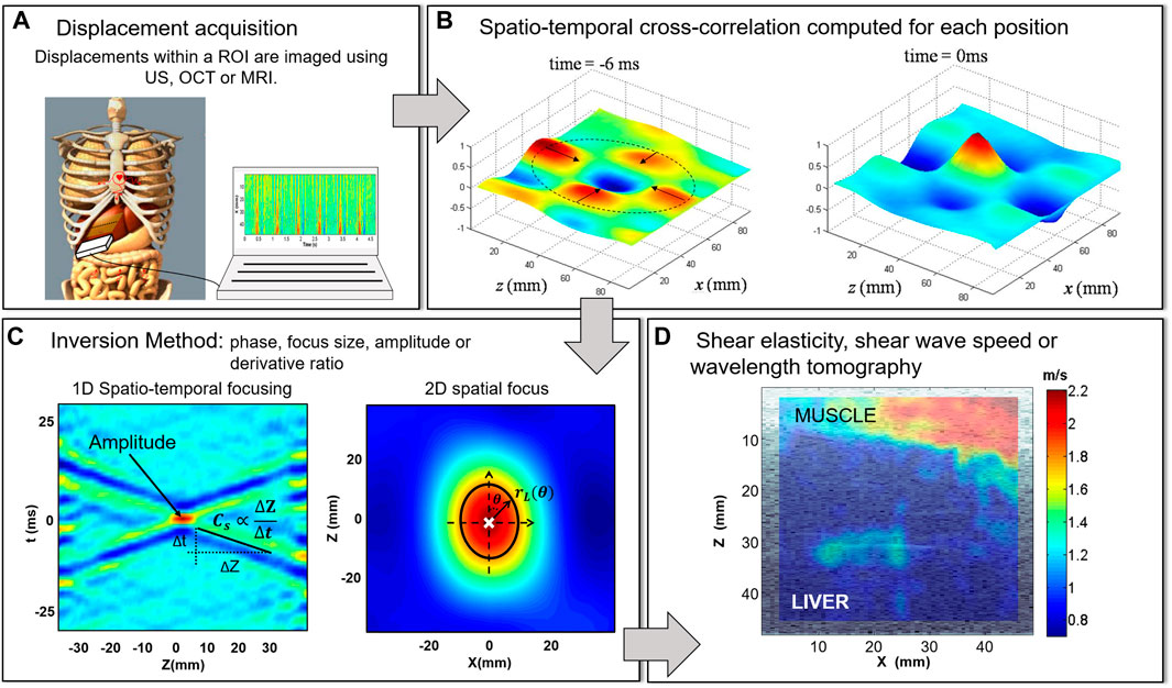
FIGURE 1. Schemmatic representation of the main steps involved in an elastography experiment based on noise correlation and time reversal (A) The first step consists in recording at least one component of the complex elastic wavefield. As an example, we present the acquisition of the physiological noise in the liver using an ultrasound (US) scanner as in [13]. (B) Then, the spatio-temporal cross-correlation field $C\left(\overrightarrow{r_o},\overrightarrow{r},t\right)$ is computed on every point $\overrightarrow{r_0}$ within the ROI. Here we show two snapshots of $C\left(\overrightarrow{r_o},\overrightarrow{r},t\right)$. At $t=-6$ ms the shear wave front (indicated by a black dashed line) converges toward $\overrightarrow{r_o}=\left(\mathrm{50,40}\right)$ mm. At the focusing time ($t=0$ ms) the direction dependent Rayleigh criterion is apprecibale by the ellipse-like shape of the focus. Adapted from [25]. (C) The third step consists in choosing the appropriate inversion method (section 3): phase, focus size, amplitude or derivative ratio method (not shown). The left panel shows the spatio-temporal focusing along the z direction for the phase method while the right panel shows the spatial focus in the $xz-$plane for the focus size method. The amplitude method consists in measuring the amplitude at the focusing point. Finally, the last step consists in repeating steps (B,C) for every point within the ROI to compute a shear elasticity, shear wave speed or shear wavelength tomography (D) Shows a passive shear wave speed tomography obtained in the human liver [13] superimposed to the echographic image in gray scale. The upper region (Z $<$ 10 mm) corresponds to the abdominal muscle while the rest of the image corresponds to the liver. The right panel of (C) was adapted from [28], with the permission of the Acoustical Society of America.

Cross-correlation methods allow to reconstruct a refocusing wavefield from an apparently random and disorganized wavefield. Figure 1B shows two snapshots of the cross-correlation field $C\left(\overrightarrow{r_o},\overrightarrow{r},t\right)$. At $t=-6$ ms the shear wave front (indicated by a black dashed line) converges toward the focusing point $\overrightarrow{r_o}=\left(\mathrm{50,40}\right)$ mm. Long time acquisitions ensured that each point within the ROI receives waves from all directions.

From the correlation field there are different independent inversion methods to image μ or equivalently c_s (Figure 1C), e.g. tracking the coherent shear wave as it focus (phase method), measuring ${\lambda }_s$ from the focus size or evaluating the vibration amplitude at the focusing point. In this section a brief overview of these and other inversion methods will be given (specific details can be found in [14, 15, 28, 29]). A summary of these methods along with its applications, advantages and references is given in Table 1.

TABLE 1

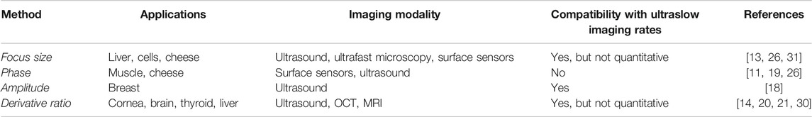
TABLE 1. Summary of the methods and applications based on noise correlation elastography.

3.1 Phase Method

The phase method consists in measuring the phase velocity $V_{\varphi }$ of the shear wave as it focus back to the source. The left panel of Figure 1C shows the evolution of the correlation field along z direction, with focusing point at $\overrightarrow{r_0}=\left(0,0\right)$mm. The cross-like shape of this figure indicates a field coming from positive and negative z direction that converges at the focusing point and then diverges. As in a classical SWE experiment, the slope of each branch of the cross is linked to $V_{\varphi }$ and hence to the shear wave speed $c_s$. Directional filters can be applied to separate each direction of propagation [4]. Then, by changing the focusing point $\overrightarrow{r_0}$ all over the ROI a shear elasticity image is constructed. This procedure was followed by Gallot et al. [13] to image the shear elasticity of a two layered phantom. The main advantage of this method is that in the far field the local phase velocity equals the shear wave velocity ($V_{\varphi }\cong c_s$). However, in the near-field ($\sim {\lambda }_s/2$) a correction to convert the phase velocity into the shear wave speed is needed. The correction factor between $V_{\varphi }$ and $c_s$ depends on the observation direction as [28]:

$V_{\varphi }=\frac{3c_s}{4}\left(1+{\gamma }_m^2\right)(5)$

where ${\gamma }_m^2$ is the direction cosine between the recorded component of the wavefield $\psi \left(\overrightarrow{r},t\right)$ and the direction of observation. Thus, near-field corrections are needed to compute the final elasticity image. For example, for ultrasound systems the recorded component of the wavefield usually coincides with the direction of the ultrasound beam (defined as z in Figure 1). Therefore, ${\gamma }_m^2=\text{cos}\left(\theta \right)$ and $V_{\varphi }=3c_s/2$ in Figure 1C. Finally, we note that for this method an ultrafast frame rate is needed in order to follow the time evolution of the cross-correlation field.

3.2 Focus Size Method

An alternative inversion method that has shown to be compatible with low imaging rates modalities is the focus size method. In a time reversal experiment with shear waves, the size of the focus is limited by diffraction to dimensions comparable to the shear wavelength. As a first approximation, one can consider that the size of the focus $\text{Δ}$, given by the width at half maximum, is related to ${\lambda }_s$ via the Rayleigh criterion for a scalar wavefield: $\text{Δ}={\lambda }_s/2$ . Given the central frequency f of the field, the shear wave speed can be retrieved via $c_s=2\text{Δ}f$. This procedure was used by Gallot et al. [13] in a passive elastography experiment. However, as described in the early works of Catheline and Benech et al. [12, 25], the focus width is direction dependent. As it focuses, the converging shear wave gives birth to near-field effects, even if it was recorded in the far-field [25]. These near-field effects (observable in Figure 1B) imply a direction dependent focus size, which is related to the dipole characteristics of the simple source for shear waves in elastodynamics [28]. Therefore, a more detailed analysis was needed to establish a quantitative relation between the focus size and ${\lambda }_s$.

In [28], by substituting the free space Green’s function for elastodynamics [39] on the right hand side of Eq. 4, the following expression relating the focus size $r_L\left(\theta \right)$ with ${\lambda }_s$ was derived:

$r_L\left(\theta \right)=\frac{{\lambda }_s}{2\pi }\sqrt{\frac{10\left(1-L\right)}{2-{\text{cos}}^2\left(\theta \right)}}=\frac{c_s}{2\pi f}\sqrt{\frac{10\left(1-L\right)}{2-{\text{cos}}^2\left(\theta \right)}}(6)$

where $r_L\left(\theta \right)$ denotes the distance from the focusing point to the contour level at which the correlation field takes a fraction $L<1$ of its maximum value (i.e. $L=1$ corresponds to the focusing point) and θ corresponds to the polar angle. The right panel of Figure 1C shows the 2D focus in a tissue mimicking phantom with $c_s=1.85$ m/s. The full black line corresponds to the contour level at −3 dB ($L=0.7$), the white cross indicates the focusing point and the distance $r_L\left(\theta \right)$ is represented by a black arrow.

Equation 6 can be used to retrieve ${\lambda }_s$ or $c_s$ if the frequency f is known. However its main drawback is that it was derived for single frequency f. The signals in the experiments are composed of multiple frequencies within a given bandwidth. Brum et al. [15] modified the above expression to include broadband signals by defining an effective frequency. This effective frequency corresponds to the frequency root mean square of the bandwidth using the power spectrum of the correlation field as weighting function. Finally, in [15] the validity of such expressions was demonstrated numerically and experimentally on a tissue-mimicking phantom consisting of two different elastic layers demonstrating the potential of the technique to quantitative shear elasticity imaging.

One advantage of the focus size method is that the time and spatial coherence are decoupled in Eq. 6. Thus, it is still possible to retrieve ${\lambda }_s$ even if the field is under sampled in the time domain, using a frame rate well below the Nyquist-Shannon sampling limit (i.e. no frequency information). This fact was shown for the first time in [12]. In this work, using 1D ultrasonic elastography, the focus size of a wavefield at 100 Hz central frequency was measured twice in an agar-gelatin phantom. The first time using ultrafast electronics (1 kHz sampling frequency) and the second one the field was under-sampled at 40 Hz rate. The focus sizes were shown to be equal for both experiments. The potential to image the elastic properties using low frame rates was later taken up in other works. In the work of Brum et al. [15], an experiment referred to as “ultraslow” (in contrast with ultrafast) was able to image the elasticity of a bilayer phantom using 10 Hz sampling frequency. In addition, the spatial resolution of the method was discussed. The conclusion is that the contour level L should be chosen as high as possible to improve the spatial resolution. Nevertheless, a trade-off exists because the presence of noise in the autocorrelation peak could make the contour level curve meaningless.

3.3 Amplitude Method

The focus size method discussed above makes use of the right-hand-side of Eq. 4. However, if the temporal frequency is unknown, as in the case of ultraslow experiments, it is not possible to convert the focus size into shear wave speed. To solve this issue, in the work of Rabin et al. [18] they chose to work out the left-hand-side of Eq. 4. As a result a quantitative expression relating the vibration amplitude at the focus (i.e., autocorrelation value) with the shear elasticity was derived. To this end, the traction $T_{jm}\left(\overrightarrow{R},\overrightarrow{r_0}\right)$ was expressed in terms of the far-field approximation of the elastodynamic Green’s function assuming that the observation points are many wavelength away from the surface. By making use of the Betty-Rayleigh identity [39] for mediums without volume sources and under the hypothesis of spatio-temporal uncorrelated sources, the shear elasticity is given by:

$\mu \left(\overrightarrow{r_0}\right)={\left[\frac{N{T}^2{A}_t}{6\pi {\mu }_0^{1/2}C\left(\overrightarrow{r_0}\right)}\right]}^{2/3}(7)$

where $C\left(\overrightarrow{r_0}\right)$ is the autocorrelation value at the focusing point $\overrightarrow{r_0}$, N is the number of traction sources, $A_t$ is the contact surface of each source and ${\mu }_0$ is the shear elasticity at the surface of the tissue. For example, in [18], they used the mean shear elasticity of breast reported in the literature as a value for ${\mu }_0$.

3.4 Derivative Ratio Method

This method was first proposed by Catheline et al. [14] and was further developed in [29] by taking into account the near field effects in the vicinity of the focusing point. This method relies on the proportionality between Eqs. 1, 2 in the presence of a diffuse field and is valid for any field obeying a wave equation. If $\psi \left(\overrightarrow{r},t\right)$ satisfies the wave equation, then, its temporal derivative $V\left(\overrightarrow{r},t\right)=\partial \psi \left(\overrightarrow{r},t\right)/\partial t$ and its spatial derivative $\xi \left(\overrightarrow{r},t\right)=\partial \psi \left(\overrightarrow{r},t\right)/\partial z$ will satisfy the same wave equation, consequently, they are time-reversal invariants. Let ${\xi }^{TR}$ and $V^{TR}$ designate the time reversal field associated to the spatial and temporal derivative, respectively. As an example, it suffices $\psi \left(\overrightarrow{r},t\right)$ to be one component of the elastic displacement field. Then, its spatial and temporal derivatives correspond to the strain and the particle velocity field, respectively.

In an ideal isotropic diffuse filed, plane wave decomposition at a given frequency allows to use the following approximations for the spatial and temporal derivatives: $\xi \approx ik\psi$ and $V\approx -i\omega \psi$. Thus, their time reversal fields can be written as: ${\xi }_0^{TR}\approx -k^2{\psi }_0^{TR}$ and $V_0^{TR}\approx -{\omega }^2{\psi }_0^{TR}$, with ${\psi }_0^{TR}={\psi }^{TR}(\overrightarrow{r_0},\overrightarrow{r_0},t=0)$. Consequently, the ratio between the time reversal fields associated to the spatial and temporal derivatives allows to retrieve the local wave speed as:

$c_s\left(\overrightarrow{r_0}\right)=\frac{\omega }{k}\propto \sqrt{\frac{V_0^{TR}}{{\xi }_0^{TR}}}(8)$

Or equivalently, for the case of ultraslow experiments the local shear wavelength can be estimated as:

${\lambda }_s\left(\overrightarrow{r_0}\right)\propto \sqrt{-\frac{{\psi }_0^{TR}}{{\xi }_0^{TR}}}(9)$

In [14] the proportionality constants for Eqs. 8, 9 were assumed to be 1 and $2\pi$, respectively, and it was demonstrated through simulations and experiments that the loss of time and spatial coherence of the recorded wavefield was not an obstacle for a tomographic reconstruction. Later, in the work of Zemzemi et al. [29] a proportionality constant of $\sqrt{1/5[2-{\text{cos}}^2\left(\theta \right)]}$ was found for Eq. 8 by introducing the near field effects described in [28].

3.5 Discussion

In this section the main advantages and drawbacks of the inversion methods presented above will be discussed. All of them rely on the presence of a diffuse field. Consequently, there is no need to control or to know the position of the shear wave source(s) nor the direction of its applied force. Moreover, reflected waves do not pose a problem as in a standard SWE experiment. This approach is advantageous in tissues where is difficult to isolate a coherent shear wave propagation from its reflections, for example, in tissues with complex boundary shape or containing several inhomogeneities. Here the more complex the wavefield the better, since waves arriving from all directions are required to improve the Green’s function retrieval from the cross-correlation. In addition, the specific shape of the shear wave sources is not relevant either.

Paradoxically, the need of a diffuse field is also the main drawback of these methods. The hypothesis of an homogeneous repartition of sources (i.e. isotropic shear wave distribution within the ROI) is needed for the exact Green’s function retrieval through cross-correlation [35]. However, this is difficult to achieve in practice. First, wave attenuation may set a limit to the diffusion process. To minimize the effects of attenuation many authors used multiple sources in their experiments [18, 29]. Second, in an internal organ, waves usually come from a given region inside/outside this organ. This may be due to the limited access when using external sources or because physiological noise comes from a preferred region within the body. For example, in the work of Gallot et al. [13] it was noted that the physiological noise recorded in the liver was highly directive coming mainly from the heart region. As result only one branch of the cross-correlation evolution used in the phase method (left panel of Figure 1C) was observed. This directivity of the wavefield can lead to biases in the reconstructed shear wave speed tomography. Nevertheless, some strategies are envisaged to overcome this drawback. One of them is to use a passive inverse filter [40] which allows an optimal spatial redistribution of the incoming energy. Another strategy is to enhance the isotropic distribution shear waves by using multiple sources. This was done in Rabin et al. [18] for the breast and in Ormachea et al. [17] in the liver by including multiple active vibration sources in the patient’s clinical bed. The use of multiple sources may also be advantageous to increase and control the frequency content of the diffuse field. The knowledge of the shear wave excitation frequency allows the shear wavelength tomography conducted with ultraslow imaging modalities to be converted into shear elasticity.

The main advantage of the phase method is a direct estimation of $V_{\varphi }$. However, for a non diffuse wavefield, where the focusing field may exhibit a preferred direction of propagation, only the projection of the wave vector along the direction of observation is measured. As a result, $V_{\varphi }$ will be overestimated. Finally, we note that this method is not compatible with low rate imaging modalities since it requires ultrafast frame rates to track the time evolution of the correlation field.

The focus size method relies in the relation between the focus size and the shear wavelength given in Eq. 6. Again, this relation is valid in the presence of a diffuse field where the Green’s function can be retrieved from cross-correlation. However, since the method uses an average value in all directions, the lack of diffusivity is not as critical as in the phase method. In addition, the size is measured around the focusing point where the signal to noise ratio is highest. Thus, the method is robust in the presence of noise. Finally, the spatial coherence is shown to be independent of the time acquisition rate. As a consequence, this method is compatible with low frame rate imaging modalities like standard ultrasound, MRI or OCT. However, at ultraslow frame rates, only the shear wavelength can be estimated because the frequency information is lost.

The amplitude method is based on the relationship between the peak of autocorrelation function and the local shear elasticity as expressed in Eq. 7. This relationship overcomes the need of knowing the frequency of the field to quantitatively measure the shear elasticity. Thus, it is fully compatible with low frame rate imaging modalities. Nevertheless, Eq. 7 was derived from the free space Green’s function. Therefore, its validity is limited in the presence of inclusions where scattering must be considered. Thus, the spatial resolution of this method as well as its quantitative value near internal boundaries or inhomogeneities needs further revision.

Strictly, the derivative ratio method does not require the presence of a diffuse field since the governing equations of this method are valid for any field obeying the wave equation. This is a great advantage compared to the other methods. However, the lack of diffusivity makes the result dependent on the specific orientation between the direction of observation and the preferred direction of the incoming energy. This method is compatible with low frame rate imaging modalities where the shear wavelength is imaged.

Viscosity is an inherent property to any biological tissue that may influence elastography methods based on noise correlation and time reversal. Although viscosity measurements were early integrated into magnetic resonance elastography [41], how to incorporate and quantify viscosity is still a matter of debate among the ultrasound-based SWE community [42]. Wave attenuation is known to mitigate the focusing quality in time reversal and cross-correlation based methods [43]. However, since spatial reciprocity remains valid even in the presence of attenuation, the best signal-to-noize ratio will be found on the focusing point at the refocusing time, i.e. time reversal acts as a spatio-temporal matched filter [44]. Consequently, in a dissipative medium the refocusing is likely to emerge from the reverberant field allowing the focus size estimation. In the work of Benech et al. [12] the influence of viscosity in the phase and focus size methods was evaluated experimentally in agarose phantoms with different Q-factors. In [12] it was found that for high Q-factors (where several reflections take place) the field can be considered as being diffuse and the mechanical properties may be accurately retrieved through both methods. Contrary, for low Q-factors the focus size method provides a more robust estimation. Moreover, as demonstrated by the numerous works and applications cited along this review, cross-correlation elastography experiments were not hindered by viscosity. Nevertheless, future works should aim to include viscosity while solving the inverse problem through the phase, focus size, amplitude or derivative ratio method.

4 Applications Of Noise Correlation And Time Reversal Elastography

The compatibility with low imaging rates modalities has led to innovative developments and new challenges in the field of multi-modality elastography. Particularly, the use of diffuse and complex wavefields has boost the concept of passive elastography to new applications involving ultrafast and ultraslow imaging modalities like ultrasound, optical methods (e.g., digital holography or OCT) and MRI.

The work of Sabra et al. [11] was the first proof of concept in the field of passive elastography based on noise correlation. In [11] they used sixteen miniature skin-mounted accelerometer placed along the vastus lateralis to measure muscular noise in the 40–55 Hz frequency band. The shear wave phase velocity dispersion was estimated from the correlation field by using a Morlet wavelet transform and by computing the slope of the shear wave arrival time for increasing sensor separation distances. The muscle’s shear elasticity and viscosity were retrieved by fitting a Voigt model to the phase velocity dispersion curve. They found that elasticity and viscosity increased with muscle load. In the work of Brum et al. [26] they also used surface sensors to record the reverberated elastic field generated by a shaker applied at the medium’s surface. In this work they used the phase and the focus size methods to measure the elasticity of a hard and a soft gelatin-based phantoms and cheese. Experiments performed in cheese allowed envision applications in the food industry, for example, evaluating the cheese ripening time.

Later, the work of Gallot et al. [13] set a milestone regarding passive elasticity imaging inside the human body. To this end they used an ultrafast ultrasound scanner to record the natural displacements in the human liver and belly muscle. To conduct the shear elasticity imaging they used the focus size method which has shown to be more robust for low signal to noise ratio. To retrieve the shear wave speed, the focus size at -6 dB was assumed to be half a shear wavelength as in the case of fluids. Nevertheless, a good agreement was obtained between the shear elasticity image and its corresponding echographic image with shear velocity values close to the ones reported by other studies. This idea was taken up in the work of Catheline et al. [14] were they used the derivative ratio method and its compatibility with low frame rate imaging modalities to conduct the first experimental in vivo demonstration of passive shear wave speed imaging using an ultrasound scanner working at a conventional frame rate. The experiment was done on the thyroid of a healthy volunteer and the ultrasonic probe was hand held during the acquisition of 800 frames at 25 Hz. Breathing and moving was prohibited during the 32 s long acquisition.

The compatibility with low rate imaging modalities boosted several innovative applications involving standard commercial ultrasound scanners, OCT and MRI systems for elasticity imaging. In the work of Zorgani et al. the derivative ratio method was used to realize a passive shear wavelength tomography in the brain using MRI [20]. The experimental validation of the sequence and method was first conducted in a calibrated tissue mimicking phantom. Then, the proof of concept was demonstrated in vivo in the brain of two healthy volunteers. Compared to other magnetic elastography techniques, this approach does not need any synchronization with the shear wave source. Later, in the work of Nguyen et al. a low frame rate spectral-domain OCT system was used to demonstrate the feasibility of a passive shear wavelength tomography on the eye of an anesthetized rat [21]. The results were cross-validated with an active elastography experiment at ultrafast frame rate. But it was not until the work of Rabin et al. [18] that quantitative elasticity imaging using ultraslow imaging systems was achieved. In their work they used the amplitude method to image in vivo the shear elasticity of healthy and tumorous breast. The B-mode images from a conventional ultrasound scanner (frame rate 30–50 Hz) were used to measure the diffuse displacement field. Since in the breast the signal to noise ratio of the physiological noise as well as the sensitivity of the algorithm used to measure the displacements are low, in this work they used an array of mechanical shakers to create the diffuse field.

Recently as in [18], many authors decided to use one or multiple shakers to generate a controlled diffuse field. In this way the signal to noise ratio inside the region of interest can be increased and the frequency content of the field can be controlled [16, 30, 31, 45]. For example, in Reverberant Shear Wave Elastography (R-SWE) a narrowband diffuse field is generated with several mechanical actuators, then, the shear wavelength is derived from the spatial autocorrelation function [16, 17, 46, 47]. Regarding the application of diffuse field interpreted within the frame of noise correlation and time reversal in the work Grasland et al. [31] a 15 kHz vibrating pipette was used to create a complex reverberated elastic field inside a cell. This novel approach was termed “cell quake elastography.” The displacement field inside the cell was imaged at 200 kHz using a microscope together with a high speed camera and the shear wavelength was estimated from the curvature of the focusing point. Elasticity images allowed identifying different cell zones (e.g. zona pellucida, cytoplasm and nucleus) in isolated and multiple cells configurations. Moreover, in [31] it was shown that elasticity decreases when the cell cytoskeleton was disrupted with cytochalasin B. This technique allow shear wave elastography at microscopic scale, opening a new research field in mechanobiology cellular properties. Moreover, in the work of Barrere et al. [30] the feasibility of monitoring high-intensity focused ultrasound (HIFU) treatments in the liver using the derivative ratio method was investigated. To this end, bovine livers were heated up to 80°C using a planar HIFU transducer and the displacements generated by a mechanical shaker were imaged with a high-frame-rate ultrasound imaging device. The formation of ablated tissue was monitored and evidenced by a tissue stiffening like in [48]. More recently, in the work of Marmin et al. [49] digital holography was used to capture a diffuse shear wave field induced by a piezoelectric actuator with a sensitivity of up to 10 nm. A shear wavelength tomography was conducted in agarose phantoms and ex vivo pork liver. Digital holography allow envisioning contact-less passive elasticity imaging with high sensitivity and spatial resolution [29]. Finally, it is important to mention that the wave-physics and algorithms developed in the frame of noise correlation and time reversal elastography are being applied in other fields of research. For example, Hillers et al. [50] analyzed seismic data with the focus size method to image the San Jacinto fault zone.

5 Conclusions and Future Directions

Throughout this short review we covered the major developments in wave-physics involving elasticity imaging using cross-correlation of a complex elastic wavefield along with its latest applications. The main advantage of this approach is its compatibility with low imaging rate modalities which has boosted the concept of passive elasticity imaging. Compared to standard SWE with an active shear wave source, a passive approach is a smart solution when shear wave generation is difficult (e.g. in well protected organs as the brain) or even dangerous, as in the case of the cornea. The various works cited along this review demonstrate the significant potential of cross-correlation elastography to become a new imaging tool in the field of multi-modality elastography. Nevertheless, it is important that future works seek to incorporate the mechanical properties inherent to tissue such as viscosity and anisotropy into the inversion methods. Moreover, cross-correlation elastography will clearly benefit from three dimensional and multiple component measurements of elastic wavefields, now possible with MRI or new 3D ultrasound imaging technologies. Over the past thirty years, different technological advances allowed SWE to be incorporated in commercial ultrasound and MRI systems, becoming a new imaging modality in clinics. Cross-correlation elastography is a very recent approach that has demonstrated its feasibility in different medical applications, however its clinical significance still needs to be demonstrated. Therefore, future works should attempt to translate this approach into clinics by proving its reproducibility, repeatability, diagnostic value and its ability to improve in vivo results. If succeeded, we believe that cross-correlation elastography will certainly become a novel multi-modality imaging tool in clinics.

Author Contributions

JB conceived the manuscript. JB and NB wrote the manuscript. JB, NB, TG, and CN revised and edited the manuscript. All authors contributed to the article and approved the submitted version.

Funding

The authors acknowledge the support of PEDECIBA-Física, Uruguay; Comisión Sectorial de Investigación Científica (CSIC), Universidad de la República, Uruguay; and Agencia Nacional de Investigación e Innovación (ANII), Uruguay.

Conflict of Interest

The authors declare that the research was conducted in the absence of any commercial or financial relationships that could be construed as a potential conflict of interest.

References

1. Nenadic IZ, Urban MW, Greenleaf JF, Gennisson JL, Bernal M, Tanter M. Ultrasound elastography for biomedical applications and medicine. Hoboken, NJ: John Wiley & Sons. (2019).

2. Sigrist RMS, Liau J, Kaffas AE, Chammas MC, Willmann JK. Ultrasound elastography: review of techniques and clinical applications. Theranostics (2017) 7:1303. doi:10.7150/thno.18650

PubMed Abstract | CrossRef Full Text | Google Scholar

3. Mariappan YK, Glaser KJ, Ehman RL. Magnetic resonance elastography: a review. Clin Anat (2010) 23:497–511. doi:10.1002/ca.21006

PubMed Abstract | CrossRef Full Text | Google Scholar

4. Deffieux T, Gennisson JL, Bercoff J, Tanter M. On the effects of reflected waves in transient shear wave elastography. IEEE Trans Ultrason Ferroelectr Freq Control (2011) 58:2032–5. doi:10.1109/TUFFC.2011.2052

PubMed Abstract | CrossRef Full Text | Google Scholar

5. Manduca A, Lake DS, Kruse SA, Ehman RL. Spatio-temporal directional filtering for improved inversion of mr elastography images. Med Image Anal (2003) 7:465–73. doi:10.1016/s1361-8415(03)00038-0

PubMed Abstract | CrossRef Full Text | Google Scholar

6. Salcudean SE, French D, Bachmann S, Zahiri-Azar R, Wen X, Morris WJ. Viscoelasticity modeling of the prostate region using vibro-elastography. Med Image Comput Comput Assist Interv (2006) 9:389–96. doi:10.1007/11866565_48

PubMed Abstract | CrossRef Full Text | Google Scholar

7. Gallichan D, Robson MD, Bartsch A, Miller KL. Tremr: table-resonance elastography with mr. Magn Reson Med (2009) 62:815–21. doi:10.1002/mrm.22046

PubMed Abstract | CrossRef Full Text | Google Scholar

8. Kanai H, Sato M, Koiwa Y, Chubachi N. Transcutaneous measurement and spectrum analysis of heart wall vibrations. IEEE Trans Ultrason Ferroelect Freq Contr (1996) 43:791–810. doi:10.1109/58.535480

CrossRef Full Text | Google Scholar

9. Konofagou EE, D'hooge J, Ophir J. Myocardial elastography--a feasibility study in vivo. Ultrasound Med Biol (2002) 28:475–82. doi:10.1016/s0301-5629(02)00488-x

PubMed Abstract | CrossRef Full Text | Google Scholar

10. Sunagawa K, Kanai H. Measurement of shear wave propagation and investigation of estimation of shear viscoelasticity for tissue characterization of the arterial wall. J Med Ultrason (2001) (2005) 32:39–47. doi:10.1007/s10396-005-0034-2

PubMed Abstract | CrossRef Full Text | Google Scholar

11. Sabra KG, Conti S, Roux P, Kuperman WA. Passive in vivo elastography from skeletal muscle noise. Appl Phys Lett (2007) 90:194101. doi:10.1063/1.2737358

CrossRef Full Text | Google Scholar

12. Benech N, Catheline S, Brum J, Gallot T, Negreira CA. 1-d elasticity assessment in soft solids from shear wave correlation: the time-reversal approach. IEEE Trans Ultrason Ferroelectr Freq Control (2009) 56:2400–10. doi:10.1109/TUFFC.2009.1328

PubMed Abstract | CrossRef Full Text | Google Scholar

13. Gallot T, Catheline S, Roux P, Brum J, Benech N, Negreira C. Passive elastography: shear-wave tomography from physiological-noise correlation in soft tissues. IEEE Trans Ultrason Ferroelectr Freq Control (2011) 58:1122–6. doi:10.1109/TUFFC.2011.1920

PubMed Abstract | CrossRef Full Text | Google Scholar

14. Catheline S, Souchon R, Rupin M, Brum J, Dinh AH, Chapelon J-Y. Tomography from diffuse waves: passive shear wave imaging using low frame rate scanners. Appl Phys Lett (2013) 103:014101. doi:10.1063/1.4812515

CrossRef Full Text | Google Scholar

15. Brum J, Catheline S, Benech N, Negreira C. Quantitative shear elasticity imaging from a complex elastic wavefield in soft solids with application to passive elastography. IEEE Trans Ultrason Ferroelectr Freq Control (2015) 62:673–85. doi:10.1109/TUFFC.2014.006965

PubMed Abstract | CrossRef Full Text | Google Scholar

16. Parker KJ, Ormachea J, Zvietcovich F, Castaneda B. Reverberant shear wave fields and estimation of tissue properties. Phys Med Biol (2017) 62:1046. doi:10.1088/1361-6560/aa5201

PubMed Abstract | CrossRef Full Text | Google Scholar

17. Ormachea J, Parker KJ, Barr RG. An initial study of complete 2d shear wave dispersion images using a reverberant shear wave field. Phys Med Biol (2019) 64:145009. doi:10.1088/1361-6560/ab2778

PubMed Abstract | CrossRef Full Text | Google Scholar

18. Rabin C, Benech N. Quantitative breast elastography from b-mode images. Med Phys (2019) 46:3001–12. doi:10.1002/mp.13537

PubMed Abstract | CrossRef Full Text | Google Scholar

19. Sabra KG, Archer A. Tomographic elastography of contracting skeletal muscles from their natural vibrations. Appl Phys Lett (2009) 95:203701. doi:10.1063/1.3254834

CrossRef Full Text | Google Scholar

20. Zorgani A, Souchon R, Dinh AH, Chapelon JY, Ménager JM, Lounis S, et al. Brain palpation from physiological vibrations using mri. Proc Natl Acad Sci USA (2015) 112:12917–21. doi:10.1073/pnas.1509895112

PubMed Abstract | CrossRef Full Text | Google Scholar

21. Nguyen TM, Zorgani A, Lescanne M, Boccara C, Fink M, Catheline S. Diffuse shear wave imaging: toward passive elastography using low-frame rate spectral-domain optical coherence tomography. J Biomed Opt (2016) 21:126013. doi:10.1117/1.JBO.21.12.126013

PubMed Abstract | CrossRef Full Text | Google Scholar

22. Campillo M, Paul A. Long-range correlations in the diffuse seismic coda. Science (2003) 299:547–9. doi:10.1126/science.1078551

PubMed Abstract | CrossRef Full Text | Google Scholar

23. Shapiro NM, Campillo M, Stehly L, Ritzwoller MH. High-resolution surface-wave tomography from ambient seismic noise. Science (2005) 307:1615–8. doi:10.1126/science.1108339

PubMed Abstract | CrossRef Full Text | Google Scholar

24. Fink M. Time reversal of ultrasonic fields. i. basic principles. IEEE Trans Ultrason Ferroelectr Freq Control (1992) 39:555–66. doi:10.1109/58.156174

PubMed Abstract | CrossRef Full Text | Google Scholar

25. Catheline S, Benech N, Brum J, Negreira C. Time reversal of elastic waves in soft solids. Phys Rev Lett (2008) 100:064301. doi:10.1103/PhysRevLett.100.064301

PubMed Abstract | CrossRef Full Text | Google Scholar

26. Brum J, Catheline S, Benech N, Negreira C. Shear elasticity estimation from surface wave: the time reversal approach. J Acoust Soc Am (2008) 124:3377–80. doi:10.1121/1.2998769

PubMed Abstract | CrossRef Full Text | Google Scholar

27. Ing RK, Quieffin N, Catheline S, Fink M. In solid localization of finger impacts using acoustic time-reversal process. Appl Phys Lett (2005) 87:204104. doi:10.1063/1.2130720

CrossRef Full Text | Google Scholar

28. Benech N, Brum J, Catheline S, Gallot T, Negreira C. Near-field effects in Green's function retrieval from cross-correlation of elastic fields: experimental study with application to elastography. J Acoust Soc Am (2013) 133:2755–66. doi:10.1121/1.4795771

PubMed Abstract | CrossRef Full Text | Google Scholar

29. Zemzemi C, Zorgani A, Daunizeau L, Belabhar S, Souchon R, Catheline S. Super-resolution limit of shear-wave elastography. Epl (2020) 129:34002. doi:10.1209/0295-5075/129/34002

CrossRef Full Text | Google Scholar

30. Barrere V, Melodelima D, Catheline S, Giammarinaro B. Imaging of thermal effects during high-intensity ultrasound treatment in liver by passive elastography: a preliminary feasibility in vitro study. Ultrasound Med Biol (2020) 45:1968-1977. doi:10.1016/j.ultrasmedbio.2020.03.019

CrossRef Full Text | Google Scholar

31. Grasland-Mongrain P, Zorgani A, Nakagawa S, Bernard S, Paim LG, Fitzharris G, et al. Ultrafast imaging of cell elasticity with optical microelastography. Proc Natl Acad Sci USA (2018) 115:861–6. doi:10.1073/pnas.1713395115

PubMed Abstract | CrossRef Full Text | Google Scholar

32. Cassereau D, Fink M. Time-reversal of ultrasonic fields. iii. theory of the closed time-reversal cavity. IEEE Trans Ultrason Ferroelectr Freq Control (1992) 39:579–92. doi:10.1109/58.156176

PubMed Abstract | CrossRef Full Text | Google Scholar

33. Fink M. Time reversal in acoustics. Contemp Phys (1996) 37:95–109. doi:10.1080/00107519608230338

CrossRef Full Text | Google Scholar

34. Gouédard P, Roux P, Campillo M, Verdel A. Convergence of the two-point correlation function toward the Green's function in the context of a seismic-prospecting data set. Geophysics (2008) 73:V47–V53. doi:10.1190/1.2985822

CrossRef Full Text | Google Scholar

35. Gouédard P, Stehly L, Brenguier F, Campillo M, Colin de Verdière Y, Larose E, et al. Cross-correlation of random fields: mathematical approach and applications. Geophys Prospect (2008) 56:375–93. doi:10.1111/j.1365-2478.2007.00684.x

CrossRef Full Text | Google Scholar

36. Roux P, Sabra KG, Kuperman WA, Roux A. Ambient noise cross correlation in free space: theoretical approach. J Acoust Soc Am (2005) 117:79–84. doi:10.1121/1.1830673

PubMed Abstract | CrossRef Full Text | Google Scholar

37. Sánchez-Sesma FJ, Pérez-Ruiz JA, Luzón F, Campillo M, Rodríguez-Castellanos A. Diffuse fields in dynamic elasticity. Wave motion (2008) 45:641–54. doi:10.1016/j.wavemoti.2007.07.005

CrossRef Full Text | Google Scholar

38. Snieder R, Wapenaar K, Wegler U. Unified Green's function retrieval by cross-correlation; connection with energy principles. Phys Rev E Stat Nonlin Soft Matter Phys (2007) 75:036103. doi:10.1103/PhysRevE.75.036103

PubMed Abstract | CrossRef Full Text | Google Scholar

39. Richards PG, Aki K. Quantitative seismology: theory and methods. San Francisco, CA: W. H. Freeman and Co. (1980). doi:10.1002/gj.3350160110

CrossRef Full Text

40. Gallot T, Catheline S, Roux P, Campillo M. A passive inverse filter for Green's function retrieval. J Acoust Soc Am (2012) 131:EL21–EL27. doi:10.1121/1.3665397

PubMed Abstract | CrossRef Full Text | Google Scholar

41. Sinkus R, Tanter M, Xydeas T, Catheline S, Bercoff J, Fink M. Viscoelastic shear properties of in vivo breast lesions measured by mr elastography. Magn Reson Imaging (2005) 23:159–65. doi:10.1016/j.mri.2004.11.060

PubMed Abstract | CrossRef Full Text | Google Scholar

42. Palmeri M, Nightingale K, Fielding S, Rouze N, Deng Y, Lynch T, et al. Rsna qiba ultrasound shear wave speed phase ii phantom study in viscoelastic media. IEEE Int Ultrason Symp (IUS) (IEEE) (2015) 1–4.

Google Scholar

43. Zhu T. Viscoelastic time-reversal imaging. Geophysics (2015) 80:A45–50. doi:10.1190/geo2014-0327.1

CrossRef Full Text | Google Scholar

44. Tanter M, Thomas JL, Fink M. Time reversal and the inverse filter. J Acoust Soc Am (2000) 108:223–34. doi:10.1121/1.429459

PubMed Abstract | CrossRef Full Text | Google Scholar

45. Beuve S, Kritly L, Callé S, Remenieras JP. Diffuse shear wave spectroscopy for soft tissue viscoelastic characterization. Ultrasonics 110 (2021) 106239. doi:10.1016/j.ultras.2020.106239

PubMed Abstract | CrossRef Full Text | Google Scholar

46. Ormachea J, Castaneda B, Parker KJ. Shear wave speed estimation using reverberant shear wave fields: implementation and feasibility studies. Ultrasound Med Biol (2018) 44:963–77. doi:10.1016/j.ultrasmedbio.2018.01.011

PubMed Abstract | CrossRef Full Text | Google Scholar

47. Zvietcovich F, Pongchalee P, Meemon P, Rolland JP, Parker KJ. Reverberant 3d optical coherence elastography maps the elasticity of individual corneal layers. Nat Commun (2019) 10:4895–13. doi:10.1038/s41467-019-12803-4

PubMed Abstract | CrossRef Full Text | Google Scholar

48. Benech N, Negreira CA. Monitoring heat-induced changes in soft tissues with 1d transient elastography. Phys Med Biol (2010) 55:1753. doi:10.1088/0031-9155/55/6/014

PubMed Abstract | CrossRef Full Text | Google Scholar

49. Marmin A, Catheline S, Nahas A. Full-field passive elastography using digital holography. Opt Lett (2020) 45:2965–8. doi:10.1364/OL.388327

PubMed Abstract | CrossRef Full Text | Google Scholar

50. Hillers G, Roux P, Campillo M, Ben‐Zion Y. Focal spot imaging based on zero lag cross‐correlation amplitude fields: application to dense array data at the San Jacinto fault zone. J Geophys Res Solid Earth (2016) 121:8048–67. doi:10.1002/2016jb013014

CrossRef Full Text | Google Scholar