Modeling Crossing Random Seas by Fully Non-Linear Numerical Simulations

Bimodal spectrum wave conditions, known as crossing seas, can produce extreme waves which are hostile to humans during oceanic activities. This study reports some new findings of the probability of extreme waves in deep crossing random seas in response to the variation of spectral bandwidth through fully non-linear numerical simulations. Two issues are addressed, namely (i) the impacts of the spectral bandwidth on the changes of extreme wave statistics, i.e., the kurtosis and crest exceedance probability, and (ii) the suitability of theoretical distribution models for accurately describing the wave crest height exceedance probability in crossing seas. The numerical results obtained by simulating a large number of crossing sea conditions on large spatial-temporal scale with a variety of spectral bandwidth indicate that the kurtosis and crest height exceedance probability will be enhanced when the bandwidth of each wave train becomes narrower, suggesting a higher probability of encountering extreme waves in narrowband crossing seas. Meanwhile, a novel empirical formula is suggested to predict the kurtosis in crossing seas provided the bandwidth is known in advance. In addition, the Rayleigh and second-order Tayfun distribution underestimate the crest height exceedance probability, while the third-order Tayfun distribution only yields satisfactory predictions for cases with relatively broader bandwidth regarding the wave conditions considered in this study. For crossing seas with narrower bandwidth, all the theoretical distribution models failed to accurately describe the crest height exceedance probability of extreme waves.

Introduction

The need for the analysis of extreme waves arises in many branches of science and engineering, while in the practice of designing the maritime structure, extreme waves are sometimes referred to as design waves with a certain return period on the basis of statistical analysis [1]. One example is so-called rogue waves featuring twice the significant height that impose substantial threats to the survivability of engineering applications and the safety of navigation activities. And their appearances are widely reported in unidirectional seas, directional seas, and crossing seas [2]. They are conventionally believed to be rare events, however, recent studies pointed out that their probability is higher than predictions based on linear theories [3]. In unidirectional seas, one of the mechanisms indicates that their formations are induced by the third-order non-linear quasi-resonant interactions, i.e., the so-called modulational instability, and their probability is associated with the Benjamin-Feir Index (BFI). To describe such extreme wave events, breather solutions to the third-order non-linear Schrödinger equation (NLSE) are suggested [4]. They have been successfully employed to reproduce extreme waves in laboratories [5–7] and numerical simulations [8, 9].

However, waves are short-crested in reality and a non-linear numerical analysis of several sets of observed field data in various European locations indicate that the main reason for the occurrence of extreme waves in directional seas is the constructive interference of elementary waves enhanced by second-order bound non-linearities rather than the modulation instability [10]. Therefore, breather models are usually not employed for the purpose to study extreme waves in directional seas. Nevertheless, ocean wave spectra, in some cases, are characterized by the coexistence of two wave systems in different propagating directions. This bimodal condition featuring two different spectral peaks is known as crossing seas. It has been recently pointed out that crossing seas are potentially hazardous and can create a freakish sea state where the probability of encountering rogue waves is high. For instance, a large percentage of ship accidents are reported due to bad weather conditions occurring in crossing sea states [11]. Some well-known examples are the Draupner wave [12], the Louis Majesty accident [13], and the tanker Prestige accident [14]. The properties of such extreme waves in crossing seas can differ significantly from those in non-crossing seas, e.g., experimental examination on the Draupner wave reveals that the onset and the type of wave breaking plays a significant role in creating steeper extreme waves in crossing seas [15]. Recently, some studies have suggested that extreme waves in crossing seas can be induced by modulational instability and can be represented by using a crossing breather wave model [16, 17]. Based on a stability analysis of the model, it is concluded that the occurrences of extreme waves in crossing seas are directly linked to (i) the angle between the propagating direction of two wave systems and (ii) the spectral bandwidth. Subsequently, many studies have been carried out to explore the effects of the crossing angles on extreme wave occurrences. For example, the stability analysis for two perturbed uniform wave trains implies that an extreme wave is the result of the balance between the large amplification factor and the large growth rate, so that angles between 10 and 30° are most probable for establishing a rogue wave sea [18], while the sideband growth reduces significantly at angles beyond about 40° and reaching complete stability at 60–80° [19]. Besides, Shukla et al. [20] extended the analysis to study the crossing of two wave groups with finite spectral bandwidth and found that the random-phased non-linearly interacting waves could propagate over long distances without being affected much by the modulational instability. For a wide enough spectral distribution, the formation of extreme waves might be completely suppressed.

In more realistic scenarios, e.g., random crossing seas featuring a bimodal JONSWAP (Joint North Sea Wave Project) shape spectrum, numerical results obtained by using the Euler equation suggest that the maximum value of the kurtosis, which is often adopted to indicate the probability of extreme waves, is achieved when the crossing angle is between 40 and 60° [21]. Besides, the numerical simulations based on the Schrödinger-type equation and fully non-linear potential theory model indicate that for crossing angle at near 90°, the non-linear interactions between the two crossing wave systems practically have negligible impact on the kurtosis [14]. More recently, Luxmoore et al. [22] investigated the effects of directional spreading and crossing angles on the statistics of wave crest heights. It is reported that the kurtosis and wave crest height exceedance probability are more sensitive to the variation of the directional spreading than the magnitude of the crossing angles between two crossing seas; it is also reported that reducing the directional spreading increases the kurtosis and the exceedance probabilities of extreme waves.

Though the crossing angles between two systems play an important role in the statistics of extreme waves, the question on the other hand about how the extreme wave statistics respond to the spectral bandwidth has not been studied so far. Hereby, we aim to address this issue through numerical modeling of the crossing random seas in deep water by using the Enhanced Spectral Boundary Integral (ESBI) model based on the fully non-linear potential theory [23]. In particular, we are interested in the crossing seas featuring symmetrical bimodal spectra consisting of two unidirectional random wave trains. Two questions will be answered in this study, namely (i) how the extreme wave statistics, i.e., the kurtosis and crest height exceedance probability, behave in response to the spectral bandwidth and (ii) whether the theoretical probability distribution, i.e., the Rayleigh distribution and second- and third-order Tayfun distributions, can be used to accurately describe the exceedance probability. In addition, a novel empirical formula will also be suggested to predict the kurtosis provided that the bandwidth is given in advance. The outcome of this study will contribute to gaining insight into extreme wave mechanisms in crossing seas and may offer solutions for optimizing the design and operations in ocean engineering practice.

Methodologies

Statistical Approach: Kurtosis and Wave Crest Exceedance Probability

The kurtosis is often employed to indicate the probability of extreme waves. Its mathematical form can be expressed by using the formula

$\begin{array}{ll}\kappa =\frac{m_4}{m_2^2},& (1)\end{array}$

where m₂ and m₄ are the second and fourth moments of the surface elevation, respectively. The Gaussian theory states that the kurtosis equals to 3. However, the non-linear effects can enhance the extreme wave probability, and therefore, kurtosis is usually larger than 3 depending on the degree of the wave non-linearities. Considering wave non-linearities up to the third order, it is reported that the kurtosis is the summation of a dynamic component due to non-linear quasi-resonant wave–wave interactions and a Stokes bound harmonic contribution [24, 25]. In a spreading sea, the former becomes a function of angular width of the directional spectrum and BFI [26, 27]. For crossing seas consisting of two unidirectional wave trains, as studied in this paper, we employ the formula for narrowband waves to predict the kurtosis [26, 28]:

$\begin{array}{ll}\tilde{\kappa }=3+\frac{\pi }{\sqrt{3}}BF{I}^2+24{\epsilon }^2,& (2)\end{array}$

where BFI is the Benjamin-Feir index given by

$\begin{array}{ll}BFI=\frac{\sqrt{2}\epsilon }{\nu }& (3)\end{array}$

with wave steepness parameter ε = k_pH_s/4 and bandwidth parameter ν, where k_p is the peak wavenumber and H_s is the significant height as 4 times the SD (short for Standard Deviation) of the surface elevations recorded at the gauges shown in Figure 1. For a narrowband wave train, its spectrum can be approximated by using the Gaussian distribution with its SD as the spectral bandwidth ν. However, the bandwidth parameter ν is not explicitly defined for crossing random seas, which will be further discussed in section Kurtosis. For simplicity, this study focuses on crossing sea featuring a symmetrical bimodal spectrum so that the method by Trulsen et al. [14] is adopted to quantify the spectral bandwidth. In other words, the bandwidth of the crossing sea is characterized by one of the bimodalities, which is denoted by its half-width at half of the spectrum peak, i.e.,

$\begin{array}{ll}\nu =(k_r-k_l)/(2k_p),& (4)\end{array}$

where k_r and k_l are corresponding wavenumbers that satisfy S(k_r) = S(k_l) = S(k_p)/2 and k_r > k_p > k_l, S(k) is the wavenumber spectrum of the unidirectional sea.

FIGURE 1

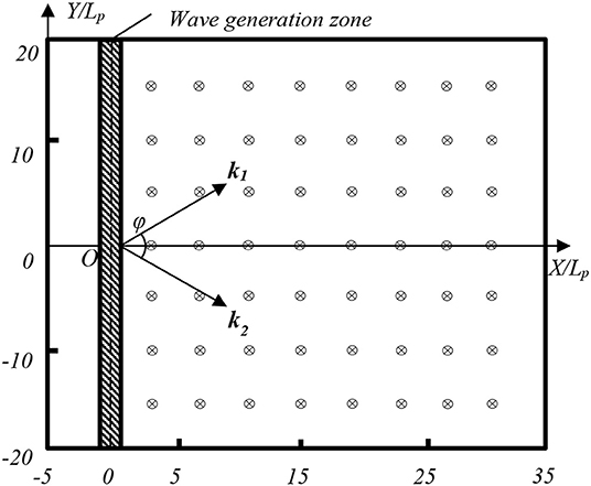
Figure 1. Plan view of the computational domain used in the numerical simulations. ⊗: location of wave probe.

On the other hand, the occurrence of extreme waves can also be depicted by the wave crest exceedance probability distribution model. For a Gaussian sea based on the linear wave theory, the exceedance probability of wave crest can be represented by the Rayleigh distribution [29]:

$\begin{array}{ll}{P}_R=exp(-8{\chi }^2),& (5)\end{array}$

where χ = H_c/H_s, H_c is the crest height measured from the mean water level to the crest peak. It is only accurate for describing the statistics for small steepness waves where the second- and higher-order non-linear effects are insignificant. However, when the wave steepness is relatively large, the second-order non-linear effects cannot be overlooked; hence, the second-order Tayfun distribution was suggested [30]:

$\begin{array}{ll}{P}_T^{(2)}=exp\left[-\frac{{(-1+\sqrt{8\sigma \chi +1})}^2}{2{\sigma }^2}\right],& (6)\end{array}$

where σ is one-third of the skewness of the free surface elevation. Furthermore, to accurately describe the exceedance probability considering third-order effects of narrowband waves, the third-order Tayfun distribution was proposed by incorporating the bandwidth coefficient in the steepness parameter [31]:

$\begin{array}{ll}{P}_T^{(3)}=P_T^{(2)}(1+\text{Λ}{\chi }^2(4{\chi }^2-1)),& (7)\end{array}$

where Λ can be approximated by using Λ = 8(κ − 3)/3 and κ is the kurtosis defined by Eq. (1) [10]. Note that though Eqs. (5)~(7) have been employed for studying wave statistics in bimodal seas [22], they are originally derived for unimodal seas, not for crossing seas. The extent to which they are able to model the distribution of crossing seas will be examined. To do so, the key parameters such as H_s, σ, and κ in Eqs. (5)~(7) are estimated by using the time histories recorded at wave gauges as illustrated in Figure 1.

Deterministic Approach: Fully Non-Linear Numerical Simulation

In this study, the ESBI method based on the fully non-linear potential theory [23] is employed to simulate crossing random seas. The details of the method are well-documented in Wang and Ma [23]. Only some key equations are briefed here for the completeness of the paper. All the dimensionless variables used in the ESBI are defined in such a way, e.g., those in length are multiplied by peak wavenumber k_p, i.e., (X, Z) = k_p (x, z), time is multiplied by peak wave frequency ω_p, i.e., T = ω_pt, velocity potential is multiplied by $k_p^2/{\omega }_p$, where x, z and t denote horizontal, vertical coordinates and time, respectively. The still water level is specified at Z=0. The free surface boundary conditions based on the fully non-linear potential theory can be reformulated as

$\begin{array}{ll}{\partial }_{T}M+AM=N& (8)\end{array}$

with each term expressed as

$\begin{array}{l}M=\left(\begin{array}{c}KF\left\{\eta \right\}\\ K\text{Ω}F\left\{\tilde{\varphi }\right\}\end{array}\right),A=\left[\begin{array}{cc}0& -\text{Ω}\\ \text{Ω}& 0\end{array}\right]\text{ and}\\ N=\left(\begin{array}{c}K\left(F\left\{V\right\}-KF\left\{\tilde{\varphi }\right\}\right)\\ \frac{K\text{Ω}}{2}F\left\{\frac{{(V+\nabla \zeta ·\nabla \tilde{\varphi })}^2}{1+|\nabla \zeta {|}^2}-|\nabla \tilde{\varphi }{|}^2\right\}\\ \end{array}\right),\end{array}$

where ϕ and η are the velocity potential and deflection of the free surface, respectively, $\tilde{\varphi }$ denotes the values of velocity potential at the surface, F{*} = ∫^*e^−iK·XdX is the Fourier transform, and F⁻¹{*} denotes the inverse transform, the wavenumber K = |K|, and the frequency $\Omega =\sqrt{K}$. Eq. (8) will be used as the prognostic equation for updating the free surface and velocity potential in the time domain, and its solution can be given by

$\begin{array}{ll}M\left(T\right)=e^{-A\left(T-T_0\right)}\left[{\displaystyle {\int }_{T_0}^T{e}^{A\left(T-T_0\right)}NdT}+M\left(T_0\right)\right],& (9)\end{array}$

where

$\begin{array}{l}{e}^{A\text{Δ}T}=\left[\begin{array}{cc}cos\text{ΩΔ}T& -sin\text{ΩΔ}T\\ sin\text{ΩΔ}T& cos\text{ΩΔ}T\\ \end{array}\right].\end{array}$

Eq. (9) can be solved by using the fifth-order Runge–Kutta method with an adaptive time step. An energy dissipation model suggested by Xiao et al. [32] is also introduced to the ESBI to suppress breaking waves, i.e.,

$\begin{array}{l}\text{Λ}=exp\left(-|\frac{K}{\beta }{|}^{\alpha }\right),\end{array}$

where α = 30 and β = 8. Its effectiveness has been demonstrated and confirmed by direct comparison against laboratory measurements.

In addition, to update $\tilde{\varphi }$ and η in the time domain, the vertical velocity V requires to be calculated at each time step. The evaluation of V can be achieved by using the boundary integral equation. It is decomposed into four parts depending on the degree of non-linearities. For clarity of the paper, the formulations for calculating V are summarized in the Appendix. The evaluation is computationally efficient, owing to the utilization of the Fast Fourier Transform. Note that the energy dissipation model is applied to both the surface elevation and velocity potential when the number of iterations for estimating the vertical velocity exceeds four times, instead of every time step as used in Xiao et al. [32]. For more details about the numerical scheme, readers can refer to Wang and Ma [23].

The ESBI model has been successfully employed to simulate the Peregrine breather and its interactions with random waves in unidirectional seas, and good agreement is achieved in comparison with the experiment measurements [9]. To verify the robustness of the ESBI model for simulating random crossing seas for the purpose in question in this study, validation is performed here by comparing with the laboratory results reported in Toffoli et al. [21]. To reproduce this crossing sea state with the same wave conditions by using the ESBI model, the computational domain covers 40-by-40 peak wavelengths and is resolved into 1,024-by-512 points in the X- and Y- directions, respectively. The selected domain size and resolution in space ensure that the Fourier modes up to 7- and 3-times peak wavenumber in the X- and Y- directions, respectively, are free of aliasing. A sensitivity test indicates that this resolution is sufficiently accurate to model the highly non-linear interactions between the two crossing wave trains for the purpose of this study. For instance, if we denote the error as the maximum difference between free surface elevation signals recorded on a probe at the same location divided by significant height, then the maximum error among all probes between the results based on the current configuration and those obtained by using 2,048-by-512 and 1,024-by-1,024 points is only about 4.3 and 5.2%, respectively. The wave generation zone is placed along the Y- direction and 5 peak wavelengths from the left boundary, while the waves are absorbed in the surrounding boundaries. The plan view of the computational domain is illustrated in Figure 1, where only part of the domain on the right-hand side is effectively used for the simulations. The wave gauges are deployed every 4 and 5 peak wavelengths in the X- and Y- directions, respectively, indicating that there are 8 × 7 = 56 gauges used in total. This will avoid the issue where using a single point observation is insufficient to investigate the extreme wave ensembles as the gauge may not always be located at the focusing point [33]. For each individual crossing sea state, four realizations are carried out by using different random number sequences as the phases for generating random waves, which is sufficient for overcoming the uncertainties due to the selection of random phases on calculating wave statistics (this will be further discussed in section Kurtosis). Meanwhile, each simulation lasts for 1,000 peak periods (equivalent to a typical 3-hour sea state), and the first 100 peak wave periods will be used for developing an established sea. We use wave surface time histories collected on the gauges where the sea state becomes equilibrium among 100–1,000 peak periods for estimating the wave statistics. It is estimated that about a total number of 10⁵ waves are recorded on the chosen gauges in the domain based on an up-cross method, which is sufficient to achieve reliable statistics. Such a method to determine the total number of waves differs from that employed by Trulsen et al. [14], where spatiotemporal correlation needs to be considered. Note that the ensemble of data measured at different locations will be used to estimate the exceedance probability. For the purpose of making a comparison with theoretical probability distribution models, the condition of homogeneity and uncorrelation should hold. We compared the wave action over space and correlations of signal collected on different gauges and found that both the conditions, i.e., homogeneity and weak correlation, are affirmed, but the results are not presented in the paper for brief.

The wave condition employs the JONSWAP spectrum with a fixed peak enhancement factor γ = 6 and wave steepness k_pH_s = 0.28. The spreading is zero and thus each individual random wave train is unidirectional. The angle between two crossing seas is fixed at φ = 40^o throughout this study, which is identified as the most hazardous angle leading to the maximum kurtosis observed in the laboratory [21]. It is worth noting that this angle is not necessarily the case for a two perturbed uniform wave train as sideband growth is observed to reduce significantly at angles beyond 40° [19]. The kurtosis is then estimated by using Eq. (1) along the X-direction (Y = 0), i.e., the mean direction, based on the simulated free surface elevation. In addition to the laboratory results, the numerical results by using the fully non-linear Higher-Order Spectrum (HOS) method reported in Toffoli et al. [21] are also included here for comparisons, all of which are summarized in Figure 2. In general, the numerical results obtained by using the ESBI depict that the kurtosis gradually grows along the X- direction and becomes stabilized near the end of the computational domain. This trend agrees very well with that observed in the laboratory, namely (i) the agreement between two curves being within the confidence interval of about ± 0.2; (ii) the difference of maximum kurtosis near the end being about 0.8%; and (iii) the difference of maximum excess kurtosis being about 8%. However, there is a big deviation from those obtained by using the HOS method. The reason may be that the configuration of the HOS model is not exactly the same as those in the laboratory, e.g., periodic boundary conditions and a smaller domain size are adopted in the simulations by using the HOS method. On the other hand, by examining the significant height along the mean direction, a reduction of about 2% is observed on the last gauge at the end of the domain in comparison with the first gauge due to the usage of the energy dissipation model to suppress breaking waves. Nevertheless, the agreement between the results obtained by using the ESBI and those from the experiment implies that the ESBI model with the current configurations can be reliably used for the purpose of this study.

FIGURE 2

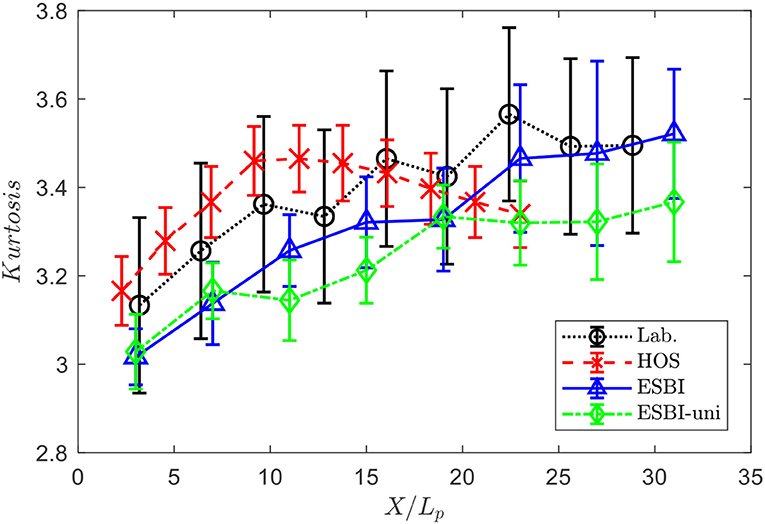
Figure 2. Kurtosis along the center line of the domain Y = 0. “Lab.”: Laboratory experiment results; “HOS”: Numerical results by using the HOS method; “ESBI”: Numerical results by using the ESBI method for crossing sea; “ESBI-uni”: Numerical results by using ESBI for non-crossing unidirectional sea.

Results and Discussions

To investigate the effects of the spectral bandwidth on extreme wave statistics in crossing seas, the JONSWAP spectrum is employed with selected values for peak enhancement factor among γ = 1 ~ 9. This range basically covers the majority of the cases from the broadband to narrowband seas [1]. Note that the larger γ is, the narrower the spectrum is. The bandwidth parameter ν is estimated based on Eq. (4) and its values are summarized in Table 1. Other configurations are the same as those explained in section Methodologies. Selected snapshots of the free surface elevation in space are extracted at the end of the simulation and they are displayed in Figure 3. It shows that at this selected time instance, the number of extreme waves observed in the crossing sea of narrow bandwidth is larger than those in the relatively broadband sea.

TABLE 1

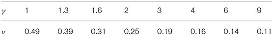
Table 1. Peak enhancement factor against spectral bandwidth.

FIGURE 3

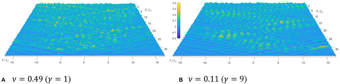
Figure 3. Selected snapshot of the free surface spatial distribution in (A) broadband sea and (B) narrowband sea.

Kurtosis

Kurtosis was selected in this study for the indication of extreme wave probability as it has been known that the non-linear four-wave interactions are one of the primary causes of rogue waves, and there is a strong correlation between the kurtosis and the strength of four-wave interactions [24]. Prior to investigating the effects of spectral bandwidth on kurtosis, it is of interest to examine whether the kurtosis is enhanced or not due to the crossing of two wave trains. For that examination, the simulations of non-crossing unidirectional random waves with k_pH_s = 0.28 and γ = 6 were performed, and the values of kurtosis along Y = 0 are shown in Figure 2. It is observed that the kurtosis for non-crossing seas grows in a similar trend to that of the crossing seas, i.e., it gradually increases along Y = 0 and becomes stabilized after propagating a distance of about 23 peak wavelengths. However, the excess part of the stabilized kurtosis near the end of the computational domain for the non-crossing seas was 36.8% smaller than that of the crossing seas. This is not surprising as the crossing sea state can produce higher steepness waves in comparison with non-crossing seas [15]. Consequently, the probability of observing extreme waves during the crossing increases; hence, the kurtosis will be enhanced. It should also be pointed out that as the crossing seas are established by two unidirectional wave trains, the kurtosis monotonically increases with distance to the asymptotic value and will not drop afterward without change of computational conditions, which is in contrast to the “overshoot” phenomenon observed in the spreading waves, where the dynamic excess kurtosis will vanish at a large distance due to energy spreads directionally [27]. In addition, to address that the kurtosis obtained by the fully non-linear model is induced by third- and higher-order non-linearities, another group of simulations of crossing seas with the wave condition k_pH_s = 0.28 and γ = 6 were performed by restricting the estimation of the vertical velocity in the ESBI model up to the second order, i.e., V = V₁ + V₂. And the second term of N in Eq. (8) is set to zero. By doing so, the non-linear effects beyond the second order were ignored in the numerical simulation, which is similar to the approach of the second-order HOS model employed in Fedele et al. [10]. The numerical results showed that the stabilized kurtosis is 3.14, which basically agreed with the theoretical prediction based on Eq. (2) without the dynamic part, i.e., $\tilde{\kappa }=3+24{\epsilon }^2\approx 3.12$. It implies that Eq. (2) without the dynamic part can be approximately used to predict the excess kurtosis due to the bound waves obtained by using the numerical model without the third- and higher-order non-linear terms. Otherwise, the kurtosis estimated using the results from the fully non-linear model exhibits larger values due to the contribution of the third- and higher-order non-linearities.

The rest of this section discusses the effects of spectral bandwidth on the kurtosis of crossing random seas. The kurtosis is firstly estimated by Eq. (1) using the surface time histories collected on probes along the center line of the domain Y = 0, and the results are summarized in Figure 4. It shows that the kurtosis increases along X-direction and is subjected to a deceleration, and then becomes stabilized toward the end of the domain. The values observed near the end of the domain are all larger than 3, indicating that the non-linearities play an important role in the formation of extreme waves in the crossing sea. In addition, the growth rate among each curve depends on the spectral bandwidth and, in general, it is faster for narrow bandwidth. Meanwhile, the stabilized kurtosis near the end of the domain also implied that narrower bandwidth yields relatively higher values of kurtosis. This finding basically agrees with that reported based on a stability analysis of crossing perturbed Stokes wave trains, which claims that narrow spectral bandwidth leads to higher amplification of the wave amplitude [18]. It should be noted that the development of unstable waves of small growth rate will be constrained by the computational domain size and so they may not develop into large waves. This is particularly important for the study of two crossing perturbed uniform wave trains [18]. However, this study aims to generate an established crossing random sea where the stabilized statistics are of interest. To demonstrate that the domain size employed in this study is sufficient for achieving stabilized statistics, a group of simulations is performed in a larger domain of 80-by-40 peak wavelengths with the same grid size for the case γ = 6. It is found that the kurtosis does not increase further beyond the maximum distance X/L_p = 31 along Y = 0. For instance, it is found that the average kurtosis within the section 23 ≤ X/L_p ≤ 31 is 3.49 in the current domain, which is very close to the average kurtosis of 3.51 within the section 23 ≤ X/L_p ≤ 47 in the larger domain. Therefore, we can justify that the kurtosis has reached the equilibrium stage within the distance 23 ≤ X/L_p ≤ 31 of the current domain.

FIGURE 4

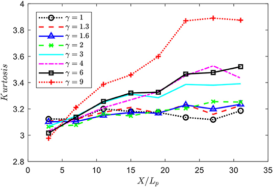
Figure 4. Kurtosis along the center line of the domain Y = 0 for cases with different bandwidth.

Apart from examining the kurtosis along the centerline, it is also important to examine the stabilized kurtosis after it reaches equilibrium. To do that, the kurtosis is estimated via Eq. (1) by using the surface time histories collected on the gauges within the section 23 ≤ X/L_p ≤ 31, and the stabilized kurtosis takes the mean value and then is averaged over four realizations. In order to demonstrate the sufficiency of the realization number, a fifth realization has also been performed and it is found that the maximum error of stabilized kurtosis between using four and five realizations is about 0.4% among all bandwidths. Therefore, four realizations are sufficient for the purpose of this study, while the results afterward are obtained based on five realizations for a more reliable analysis. The results of stabilized kurtosis against the spectral bandwidth are summarized in Figure 5. The figure shows that the stabilized kurtosis decreases as the spectral bandwidth becomes wider. Furthermore, it is also noted that the variation of the stabilized kurtosis drops faster for narrower bandwidth and is subject to a deceleration toward broader bandwidth. Its maximum corresponding to the narrowest bandwidth, i.e., ν = 0.11 (γ = 9), is about 3.88, which is much larger than 3, i.e., the Gaussian sea indicator. It implies that the probability of extreme waves due to the non-linear interactions between two crossing seas can be significant in the area where crossing is evident. And the chance of encountering an extreme wave is much higher than the predicted probability based on the linear theory.

FIGURE 5

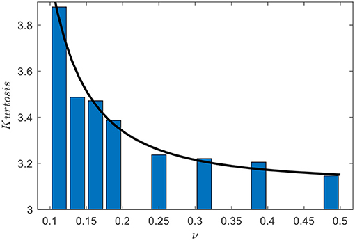
Figure 5. Average kurtosis against spectral bandwidth. Bars represent the values estimated by using Eq. (1); Lines represent fitted results by Eq. (11).

Next, to predict the kurtosis for crossing seas provided that the bandwidth is given, the relationship between kurtosis and spectral bandwidth is to be established. However, Eqs. (2)~(4) cannot be directly used in crossing seas as there is no unique way to quantify the bandwidth. For example, many studies have suggested estimating the spectral bandwidth for unidirectional seas by using, e.g., the peakedness parameter introduced by Goda [34], zeroth, first and second moment of the spectrum [29], renormalized SD of the spectrum [22, 24], or the half-width at half the peak value of the spectrum [14]. Each method produces bandwidth values in a certain range and they can be empirically converted to each other [24, 35]. Nevertheless, to achieve this goal, here, we refer to Eqs. (2)~(4) and examine whether they can be improved to approximate the values of kurtosis reported in Figure 5. According to Eq. (2), as the wave steepness and angle of crossing are fixed, one expects the variation of the predicted excess kurtosis is in proportion to the inverse of ν², i.e.,

$\begin{array}{ll}\tilde{\kappa }-\sigma \propto \frac{1}{{\nu }^2},& (10)\end{array}$

where σ is expected to be a constant larger than 3 as it includes the non-linear Stokes contribution. Based on that, the least squares method is performed to fit the values of kurtosis in Figure 5, and the relationship between kurtosis and spectral bandwidth can then be established by using the following formula:

$\begin{array}{ll}{\kappa }^{\prime }=3.116+\frac{0.009}{{\nu }^2},X/L_p\ge 21& (11)\end{array}$

The curve of fitted values κ′ is displayed in Figure 5, which agrees very well with those calculated directly from using the fully non-linear simulation results. The suggested formula has successfully captured the variation of the kurtosis subject to the changes of the bandwidth, while the maximum error is about 5%. The good agreement reveals that Eq. (11) modified based on Eqs. (2)~(4) works very well for the cases being studied here. Heuristically, the usage of the spectral bandwidth for predicting the kurtosis may be extended in crossing seas with wave conditions not limited in this study. Note that Eq. (11) can only be used for predicting the stabilized kurtosis in the region where waves attain equilibrium or are fully developed. The variation of kurtosis during the translational stage is not the focus of this study as it is induced by the unrealistic assumption of the initial Gaussian wave field [27] for wave generation and does not provide practical value.

Wave Crest Exceedance Probability

In this section, the exceedance probability of the crest height is estimated by using the surface elevation time histories collected on gauges within the section 23 ≤ X/L_p ≤ 31 over five realizations with a down-crossing method performed in the time domain (with a sampling rate of 40 points per peak period) and comparisons are made against the theories based on Eqs. (5)~(7). It should be pointed out that such a way to ensemble crest height over spatial measurements is equivalent to the averaged exceedance probability over the selected gauges. Note that the values of kurtosis as used by Eq. (7) are those presented in Figure 5, i.e., those estimated directly from using the fully non-linear simulation results. It means that the theoretical results by Eq. (7) consider a certain degree of fully non-linear effects. To verify the effects of bandwidth on the exceedance probability, the numerical results are summarized and displayed in Figure 6. It indicates that the probability of the extreme waves as described by the tail of the distribution generally increases as the spectral bandwidth becomes narrower. This is consistent with the findings regarding the kurtosis in section Kurtosis. It is also depicted in Figure 6, when the spectral bandwidth becomes extremely narrow, e.g., ν ≤ 0.19, the exceedance probability obtained from the numerical results starts to exhibit a higher tail moving toward a straight asymptote in the semi-logarithm scale. This is unusual and worth to be further investigated comprehensively. Nevertheless, it can be concluded that the probability of observing an extreme wave in the crossing sea is enhanced if the spectral bandwidth reduces.

FIGURE 6

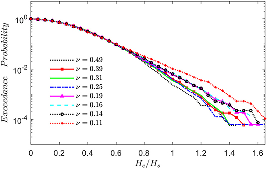
Figure 6. Wave crest exceedance probability estimated by using fully non-linear numerical results.

In addition, to discuss the suitability of theoretical distribution models for describing the crest height exceedance probability, the predictions based on Eqs. (5)~(7) and those obtained from numerical results are summarized in Figure 7. It can be noted that both the Rayleigh distribution and second-order Tayfun distribution underestimate the wave crest exceedance probability in all the cases being studied here, which is also reported in a study with experiments conducted in a laboratory [22]. Therefore, it can be concluded that the Rayleigh distribution based on the linear wave theory and the Tayfun distribution of second-order cannot be used to accurately describe the crest exceedance probability in crossing sea state with the wave conditions discussed in this study. This basically agrees with the findings by Fedele et al. [36] using space-time measurements in crossing sea states consisting of swell and wind waves. On the other hand, for relatively wider spectral bandwidth, as shown in Figures 7A,B, the third-order Tayfun distribution is generally in good agreement with the numerical results, though slightly overestimates the probability in the range H_c/H_s < 1. However, the discrepancy between the numerical results and third-order Tayfun theoretical distribution becomes evident for relatively narrower bandwidth as shown in Figures 7C,D. In particular, the difference becomes dramatic in the range H_c/H_s > 1.2, which is often used as one of the criteria to justify whether an extreme is a rogue wave (the other condition H/H_s > 2 must also be met to be identified as a rogue wave, where H is the crest to trough height). For example, it is noticed that for those cases with relatively narrower bandwidth, the third-order Tayfun distribution significantly underestimates the exceedance probability at the tail of the distribution. Therefore, the third-order Tayfun distribution may not be suitable for studying the crest exceedance probability for the crossing wave conditions with narrow bandwidths, even for the average peakedness condition of a JONSWAP sea, i.e., γ = 3.

FIGURE 7

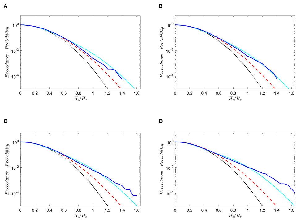
Figure 7. Wave crest exceedance probability. “···”: P_R, Rayleigh distribution; “—“:$P_T^{(2)}$, second-order Tayfun distribution; “·−·−·”: $P_T^{(3)}$, third-order Tayfun distribution; “–”: Numerical results based on ESBI. (A) ν = 0.49 (γ = 1). (B) ν = 0.31 (γ = 1.6). (C) ν = 0.19 (γ = 3). (D) ν = 0.11 (γ = 9).

Conclusions

This study discusses the effects of spectral bandwidth on the extreme wave statistics in deep crossing seas, in particular, the kurtosis and wave crest exceedance probability, through fully non-linear numerical simulations on a large spatial-temporal scale of 40 × 40 peak wavelengths in domain size and 1,000 peak periods in time. Each of the two random wave trains is unidirectional based on the JONSWAP spectrum with a peak enhancement factor in the range 1–9. The free surface time histories are collected on selected wave probes deployed in the computational domain where the waves attain equilibrium and are used for reliable estimation of the kurtosis and exceedance probability. Verification of the numerical model is performed against laboratory experiments while the robustness of the numerical model is demonstrated by the good agreement observed with measurements with a confidence interval of ±0.2 for averaged kurtosis, while errors of maximum kurtosis and maximum excess kurtosis were about 0.8 and 8%, respectively.

The results reveal that the excess part of the stabilized kurtosis for the non-crossing seas is about 40% smaller than that of the crossing seas. This is due to the fact that the crossing sea state creates higher steepness waves [15], and the probability of observing extreme waves increases as a consequence, hence, enhancing the kurtosis in the crossing seas. Besides, it is concluded that the kurtosis will become smaller when the spectral bandwidth of each individual random wave train in crossing seas increases, and its variation subjects to a deceleration toward broader bandwidth. The maximum kurtosis observed in this study is about 3.88, which is much higher than the Gaussian sea indicator, i.e., κ = 3. It is evidenced that the non-linearities play an important role in the enhancement of the kurtosis in crossing seas. Besides, a novel empirical formula for predicting the stabilized kurtosis by using the spectral bandwidth is proposed where the coefficients are derived through fitting the numerical values. The formula suggests that the excess kurtosis is proportional to the inverse of the square of bandwidth. Meanwhile, the good agreement between the fitted and numerical results with a maximum error of about 5% is encouraging, which implies that the suggested formula has the potential to be extended for other wave conditions not considered in this study, but it requires careful calibration.

Furthermore, the study also shows that the crest height exceedance probability of extreme waves grows as a result of narrower bandwidth. Comparisons between the numerical results and theoretical distributions, i.e., the Rayleigh distribution, second- and third-order Tayfun distribution, are also carried out. It is found that the Rayleigh and second-order Tayfun distribution significantly underestimate the exceedance probability regardless of the spectral bandwidth. Thus, neither of them can be used to accurately predict the crest exceedance probability in crossing seas if the wave conditions are similar to those reported in this study, i.e., initial steepness k_pH_s = 0.28 and crossing angle φ = 40^o. Meanwhile, the third-order Tayfun distribution can successfully describe the exceedance probability for cases of relatively broader bandwidth, e.g., γ ≤ 1.6; however, it underestimates the tail of the distribution when the bandwidth becomes narrower. Therefore, the suitability of third-order Tayfun distribution for crossing seas depends on the magnitude of the bandwidth, which needs to be investigated quantitatively. However, these conclusions are arrived at using the results for crossing seas. This does not negate the suitability of their application in non-crossing (or uni-modal) seas.

Nevertheless, it should be noted that this study only covers some cases in a broad class of situations, e.g., the crossing sea in this study features a symmetrical bimodal spectrum, which is composed of two unidirectional random wave trains that are identical in terms of the significant height, peak wavenumber, and bandwidth. Therefore, the conclusions above hold only for the cases reported in this study and may not be true for other cases beyond the wave conditions considered here, namely the initial steepness k_pH_s not being equal to 0.28, the crossing angle not being 40^o, spreading angle of each wave train not being 0, and the spectral shape not being able to be described by the JONSWAP spectrum. Studies will be carried out in the future to investigate the extreme wave properties in two crossing seas subject to the variation of other wave parameters such as wave steepness, crossing angle, etc., and spreading will also be considered in order to identify the most influential factor on the extreme wave statistic. The correlation between the wave steepness and crossing angle needs to be considered as well, as the integral steepness varies largely with the crossing condition subject to cyclonic winds [37]. Note that the scaling should be taken into consideration for predicting the variation of kurtosis during the translational stage. Eq. (11) cannot be used for this purpose. That being said, this formula is an implication that the kurtosis is inversely proportional to the spectral bandwidth. In addition, Ruban [38], in a recent study, pointed out that the formation of extreme waves also depends on the orientation of the wavefronts to the direction of the group, while the highest amplification happens at about 18–28° degrees. To address this issue in crossing seas, the effects of various angles between the wavefront and group direction of each individual random wave train on excitation of extreme waves during crossing will also be taken into consideration in the future study.

Data Availability Statement

The raw data supporting the conclusions of this article will be made available by the authors, without undue reservation.

Author Contributions

JW was responsible for conceptualization, methodology, analysis, and writing. QM was responsible for data curation, writing, and editing. SY was responsible for writing and reviewing. BL was responsible for reviewing. All authors contributed to the article and approved the submitted version.

Funding

JW and BL show gratitude to the sponsorship provided by NSFC, China (51679223, 51739010). QM and SY acknowledge the financial support of EPSRC, UK (EP/L01467X/1, EP/T00424X/1, EP/T026782/1), and DST-UKIERI project (DST-UKIERI-2016-17-0029).

Conflict of Interest

The authors declare that the research was conducted in the absence of any commercial or financial relationships that could be construed as a potential conflict of interest.

Acknowledgments

JW acknowledges the host of Prof. Philip L.-F. Liu at Faculty of Engineering, National University of Singapore, where this research was conducted. The authors would like to thank the very insightful comments of three reviewers.

Supplementary Material

The Supplementary Material for this article can be found online at: https://www.frontiersin.org/articles/10.3389/fphy.2021.593394/full#supplementary-material

References

1. Goda Y. Random Seas and Design of Maritime Structures. 3rd edn. Singapore: World scientific (2010).

Google Scholar

2. Kharif C, Pelinovsky E, Slunyaev A. Rogue Waves in the Ocean. Berlin: Springer-Verlag (2009).

Google Scholar

3. Ruban V, Kodama Y, Ruderman M, Dudley J, Grimshaw R, McClintock PVE, et al. Rogue waves–towards a unifying concept?: Discussions and debates. Eur Phys J Special Top. (2010) 185:5–15. doi: 10.1140/epjst/e2010-01234-y

CrossRef Full Text | Google Scholar

4. Akhmediev N, Ankiewicz A, Taki M. Waves that appear from nowhere and disappear without a trace. Phys Lett A. (2009) 373:675–8. doi: 10.1016/j.physleta.2008.12.036

CrossRef Full Text | Google Scholar

5. Chabchoub A, Hoffmann NP, Akhmediev N. Rogue wave observation in a water wave tank. Phys Rev Lett. (2011) 106:204502. doi: 10.1103/PhysRevLett.106.204502

PubMed Abstract | CrossRef Full Text | Google Scholar

6. Chabchoub A, Hoffmann N, Onorato M, Slunyaev A, Sergeeva A, Pelinovsky E, et al. Observation of a hierarchy of up to fifth-order rogue waves in a water tank. Phys Rev E. (2012) 86:056601. doi: 10.1103/PhysRevE.86.056601

PubMed Abstract | CrossRef Full Text | Google Scholar

7. Chabchoub A. Tracking breather dynamics in irregular sea state conditions. Phys Rev Lett. (2016) 117:144103. doi: 10.1103/PhysRevLett.117.144103

PubMed Abstract | CrossRef Full Text | Google Scholar

8. Slunyaev A, Pelinovsky E, Sergeeva A, Chabchoub A, Hoffmann N, Onorato M, et al. Super-rogue waves in simulations based on weakly nonlinear and fully nonlinear hydrodynamic equations. Phys Rev E. (2013) 88:012909. doi: 10.1103/PhysRevE.88.012909

PubMed Abstract | CrossRef Full Text | Google Scholar

9. Wang J, Ma QW, Yan S, Chabchoub A. Breather rogue waves in random seas. Phys Rev Appl. (2018) 9:014016. doi: 10.1103/PhysRevApplied.9.014016

CrossRef Full Text | Google Scholar

10. Fedele F, Brennan J, Ponce de León S, Dudley J, Dias F. Real world ocean rogue waves explained without the modulational instability. Sci Rep. (2016) 6:27715. doi: 10.1038/srep27715

PubMed Abstract | CrossRef Full Text | Google Scholar

11. Toffoli A, Lefèvre JM, Monbaliu J, Bitner-Gregersen E. Dangerous sea-states for marine operations. In: Proceedings of the 14th International Offshore and Polar Engineering Conference. Toulon (2004).

Google Scholar

12. Adcock TAA, Taylor PH, Yan S, Ma QW, Janssen PAEM. Did the draupner wave occur in a crossing sea? Proc R Soc London A: Mathematical Phys Eng Sci. (2011) 467:3004–21. doi: 10.1098/rspa.2011.0049

CrossRef Full Text | Google Scholar

13. Cavaleri L, Bertotti L, Torrisi L, Bitner-Gregersen E, Serio M, Onorato M. Rogue waves in crossing seas: The Louis Majesty accident. J Geophys Res Oceans. (2012) 117:1–8. doi: 10.1029/2012JC007923

CrossRef Full Text | Google Scholar

14. Trulsen K, Nieto-Borge JC, Gramstad O, Aouf L. Crossing sea state and rogue wave probability during the prestige accident. J Geophys Res Oceans. (2015) 120:7113–36. doi: 10.1002/2015JC011161

CrossRef Full Text | Google Scholar

15. McAllister ML, Draycott S, Adcock TAA, Taylor PH, van den Bremer TS. Laboratory recreation of the Draupner wave and the role of breaking in crossing seas. J Fluid Mech. (2019) 860:767–86. doi: 10.1017/jfm.2018.886

CrossRef Full Text | Google Scholar

16. Onorato M, Osborne AR, Serio M. Modulational instability in crossing sea states: a possible mechanism for the formation of freak waves. Phys Rev Lett. (2006) 96:014503. doi: 10.1103/PhysRevLett.96.014503

PubMed Abstract | CrossRef Full Text | Google Scholar

17. Shukla PK, Kourakis I, Eliasson B, Marklund M, Stenflo L. Instability and evolution of nonlinearly interacting water waves. Phys Rev Lett. (2006) 97:094501. doi: 10.1103/PhysRevLett.97.094501

PubMed Abstract | CrossRef Full Text | Google Scholar

18. Onorato M, Proment D, Toffoli A. Freak waves in crossing seas. Eur Phys J Special Topics. (2010) 185:45–55. doi: 10.1140/epjst/e2010-01237-8

CrossRef Full Text | Google Scholar

19. Steer JN, McAllister ML, Borthwick AG, Van Den Bremer TS. Experimental observation of modulational instability in crossing surface gravity wavetrains. Fluids. (2019) 4:105. doi: 10.3390/fluids4020105

CrossRef Full Text | Google Scholar

20. Shukla PK, Marklund M, Stenflo L. Modulational instability of nonlinearly interacting incoherent sea states. JETP Lett. (2007) 84:645–9. doi: 10.1134/S0021364006240039

CrossRef Full Text | Google Scholar

21. Toffoli A, Bitner-Gregersen EM, Osborne AE, Serio E, Monbaliu J, Onorato M. Extreme waves in random crossing seas: laboratory experiments and numerical simulations. Geophys Res Lett. (2011) 38:6. doi: 10.1029/2011GL046827

CrossRef Full Text | Google Scholar

22. Luxmoore JF, Ilic S, Mori N. On kurtosis and extreme waves in crossing directional seas: a laboratory experiment. J Fluid Mech. (2019) 876:792–817. doi: 10.1017/jfm.2019.575

CrossRef Full Text | Google Scholar

23. Wang J, Ma QW. Numerical techniques on improving computational efficiency of spectral boundary integral method. Int J Numer Methods Eng. (2015) 102:1638–69. doi: 10.1002/nme.4857

CrossRef Full Text | Google Scholar

24. Janssen PA. Nonlinear four-wave interactions and freak waves. J Phys Oceanogr. (2003) 33:863–84. doi: 10.1175/1520-0485(2003)33&lt;863:NFIAFW&gt;2.0.CO;2

CrossRef Full Text | Google Scholar

25. Janssen PA. On some consequences of the canonical transformation in the Hamiltonian theory of water waves. J Fluid Mech. (2009) 637:1–44. doi: 10.1017/S0022112009008131

CrossRef Full Text | Google Scholar

26. Mori N, Janssen PA. On kurtosis and occurrence probability of freak waves. J Phys Oceanogr. (2006) 36:1471–83. doi: 10.1175/JPO2922.1

CrossRef Full Text | Google Scholar

27. Fedele F. On the kurtosis of deep-water gravity waves. J Fluid Mech. (2015) 782:25–36. doi: 10.1017/jfm.2015.538

CrossRef Full Text | Google Scholar

28. Janssen PA, Bidlot JR. On the Extension of the Freak Wave Warning System and Its Verification. s.l.:European Centre for Medium-Range Weather Forecasts, Reading (2009).

Google Scholar

29. Longuet-Higgins MS. On the joint distribution of wave periods and amplitudes in a random wave field. Proc R Soc Lond. (1983) 389:241–58. doi: 10.1098/rspa.1983.0107

CrossRef Full Text | Google Scholar

30. Tayfun M. Narrow-band nonlinear sea waves. J Geophys Res Oceans. (1980) 85:1548–52. doi: 10.1029/JC085iC03p01548

CrossRef Full Text | Google Scholar

31. Tayfun MA, Fedele F. Wave-height distributions and nonlinear effects. Ocean Eng. (2007) 34:1631–49. doi: 10.1016/j.oceaneng.2006.11.006

CrossRef Full Text | Google Scholar

32. Xiao W, Liu Y, Wu G, Yue DKP. Rogue wave occurrence and dynamics by direct simulations of nonlinear wave-field evolution. J Fluid Mech. (2013) 720:357–92. doi: 10.1017/jfm.2013.37

CrossRef Full Text | Google Scholar

33. Benetazzo A, Ardhuin F, Bergamasco F, Cavaleri L, Guimarães PV, Schwendeman M, et al. On the shape and likelihood of oceanic rogue waves. Sci Rep. (2017) 7:8276. doi: 10.1038/s41598-017-07704-9

PubMed Abstract | CrossRef Full Text | Google Scholar

34. Goda Y. Numerical experiments on wave statistics with spectral simulation. Report Port Harbour Res Inst. (1970) 9:3–57.

Google Scholar

35. Mori N, Onorato M, Janssen PA. On the estimation of the kurtosis in directional sea states for freak wave forecasting. J Phys Oceanogr. (2011) 41:1484–97. doi: 10.1175/2011JPO4542.1

CrossRef Full Text | Google Scholar

36. Fedele F, Benetazzo A, Gallego G, Shih PC, Yezzi A. Space–time measurements of oceanic sea states. Ocean Model. (2013) 70:103–15. doi: 10.1016/j.ocemod.2013.01.001

CrossRef Full Text | Google Scholar

37. Holthuijsen LH, Powell MD, Pietrzak JD. Wind and waves in extreme hurricanes. J Geophys Res Oceans. (2012) 117:C09003. doi: 10.1029/2012JC007983

CrossRef Full Text | Google Scholar

38. Ruban VP. Enhanced rise of rogue waves in slant wave groups. JETP Lett. (2011) 94:177–81. doi: 10.1134/S0021364011150100

CrossRef Full Text | Google Scholar