A Vector Series Solution for a Class of Hyperbolic System of Caputo Time-Fractional Partial Differential Equations With Variable Coefficients

In this paper, we introduce a series solution to a class of hyperbolic system of time-fractional partial differential equations with variable coefficients. The fractional derivative has been considered by the concept of Caputo. Two expansions of matrix functions are proposed and used to create series solutions for the target problem. The first one is a fractional Laurent series, and the second is a fractional power series. A new approach, via the residual power series method and the Laplace transform, is also used to find the coefficients of the series solution. In order to test our proposed method, we discuss four interesting and important applications. Numerical results are given to authenticate the efficiency and accuracy of our method and to test the validity of our obtained results. Moreover, solution surface graphs are plotted to illustrate the effect of fractional derivative arrangement on the behavior of the solution.

1 Introduction

Many natural phenomena have been modeled through partial differential equations (PDEs), especially in physics, engineering, chemistry, and biology, as well as in humanities [1, 2]. A wide range of PDEs can be classified under the name of hyperbolic PDEs that have the following general form [2–6]:

$u_t\left(x,t\right)=a\left(x,t\right)u_x\left(x,t\right)+b\left(x,t\right)u\left(x,t\right)+f\left(x,t\right),x\in \mathrm{\Im },t>0,(1)$

subject to the following initial condition:

$u\left(x,0\right)=u_0\left(x\right).(2)$

The equations of compressible fluid flow and the Euler equations are examples of PDEs that can be reduced to hyperbolic PDEs when the effects of viscosity and heat conduction are neglected [6]. In addition, many mathematical models are appearing as hyperbolic systems of PDEs that have the following general form:

$U_t\left(x,t\right)=A\left(x,t\right)U_x\left(x,t\right)+B\left(x,t\right)U\left(x,t\right)+F\left(x,t\right),x\in \mathrm{\Im },t\ge 0,(3)$

subject to

$U\left(x,0\right)=U_0\left(x\right),(4)$

where $U\left(x,t\right),F\left(x,t\right)\in M_{n\times 1},n\in \mathrm{\mathbb{N}}$ are vector functions of two variables x and t,$U_0\left(x\right)\in M_{n\times 1}$ is a vector function of x, $A\left(x,t\right),B\left(x,t\right)\in M_{n\times n}$ are matrix functions of two variables x and t, and $A\left(x_0,t_0\right)$ is diagonalizable with real eigenvalues for every $\left(x_0,t_0\right)\in \mathrm{\Im }\times \left[0,\infty \right)$. The system in Eqs 3, 4 is said to be strictly hyperbolic if the eigenvalues of $A\left(x_0,t_0\right)$ are all distinct, whereas it is said to be elliptic at a point $\left(x_0,t_0\right)$ if none of the eigenvalues of $A\left(x_0,t_0\right)$ are real for every $\left(x_0,t_0\right)\in \mathrm{\Im }\times \left[0,\infty \right)$.

In recent decades, many mathematical models have been reformulated using the concept of fractional calculus because they are found to reflect the phenomenon that has been modeled in a more precise and realistic way by replacing the ordinary derivative with a fractional derivative (FD) of the model. The concept of fractional calculus dates back to the 17th century [7, 8] and has recently gained considerable interest because of its extensive use in widespread fields, for instance, engineering, biological, chemical, and applied physics such as in nonlinear oscillation, waves, and diffusion as we mentioned [7–13]. In fact, from that date until now, there are many definitions of the FD. The most popular definition is the Caputo FD that is denoted and defined as [7, 8]

${\mathfrak{D}}_t^{\alpha }u\left(x,t\right)=\{\begin{array}{cc}{J}_t^{m-\alpha }{\partial }_t^{m}u\left(x,t\right),& \begin{array}{c}m-1<\alpha <m,\end{array}\\ {\partial }_t^{m}u\left(x,t\right),& \alpha =m,\end{array},t>t_0\ge 0,(5)$

where $m\in \mathrm{\mathbb{N}}$ and $J_t^{\alpha }$ is the Riemann–Liouville fractional integral operator (R-LFIO) of order $\alpha >0$ with respect to $t\ge t_0\ge 0$, which is defined by

$J_t^{\alpha }u\left(x,t\right)=\frac{1}{\text{Γ}\left(\alpha \right)}{\displaystyle {\int }_{t_0}^t{\left(t-\tau \right)}^{\alpha -1}u\left(x,\tau \right)d\tau },t>\tau >t_0\ge 0.(6)$

For more details about the properties of the two previous definitions, readers can refer to the references [7–12]. The most useful properties that we need in this research are

$J_t^{\alpha }{\left(t-t_0\right)}^{\mu }=\frac{\Gamma (\mu +1)}{\Gamma (\mu +\alpha +1)}{\left(t-t_0\right)}^{\mu +\alpha },\mu >-1,t\ge t_0\ge 0,(7)$

$J_t^{\alpha }\lambda =\frac{\lambda }{\Gamma (\alpha +1)}{\left(t-t_0\right)}^{\alpha },\lambda isaconstant,(8)$

${\mathfrak{D}}_t^{\alpha }{\left(t-t_0\right)}^{\mu }=\{\begin{array}{cc}\frac{\Gamma (\mu +1)}{\Gamma (\mu -\alpha +1)}{\left(t-t_0\right)}^{\mu -\alpha },& \mu \notin \left\{\mathrm{0,1,2},\dots ,m-1\right\}\\ 0& \mu \in \left\{\mathrm{0,1,2},\dots ,m-1\right\}\end{array},(9)$

${\mathfrak{D}}_t^{\alpha }\lambda =0,\lambda isaconstant.(10)$

As mentioned, the definition of Caputo is one of the most important definitions of the FD, since it was and still is an appropriate and effective tool in the modeling of many natural phenomena in all sciences and fields. For example, but not limited to, the definition of Caputo has recently been used to construct a mathematical model to illustrate the impacts of deforestation on wildlife species [13], in a fractional investigation of bank data [14], to model the spread of hookworm infection [15], and newly to model and analyze the dynamics of novel coronavirus (COVID-19) [16].

It is difficult to find exact solutions (ESs) for the fractional differential and integral equations; for this reason, analytical and numerical methods are usually used to find approximate solutions (ASs) for those equations. In recent decades, many methods have been used to find analytical and numerical solutions for fractional differential and integral equations such as the variational iteration method [17], the Adomian decomposition method [18], the homotopy perturbation method [17], the homotopy analysis method, the fractional transform method [19], Green’s function method [20], and other methods [21, 22].

In the last five years, the residual power series method (RPSM) has achieved an advanced rank among the methods used to find ASs for many fractional differential and integral equations. It has been used in determining ESs and ASs for many equations such as homogeneous and non-homogeneous time- and space-fractional telegraph equation [23], time-fractional Boussinesq-type and space-fractional Klein–Gordon–type equations [24], fractional multi-pantograph system [25], space- and time-fractional linear and nonlinear KdV–Burgers equation [26], multi-energy groups of neutron diffusion equations [27], and other equations. The RPSM is characterized by its ease and speed in finding solutions for equations in the form of a power series. In fact, the RPSM is a mechanism for finding the coefficients of the fractional power series (FPS) without having to find a recurrence relation that we normally obtain from equating the corresponding coefficients in the series. The RPSM is a good alternate proceeding for gaining analytic solutions for fractional PDEs.

Despite all the features we mentioned about the RPSM, we will present in this paper a major modification to the method. We use the concept of limit at infinity instead of the concept of FD in determining the coefficients of the power series solution (SS). As is well known, finding an FD manually is not easy and sometimes takes tens of minutes when it is calculated by software packages, while calculating the limit is much easier than calculating the FD manually and faster by compute. Indeed, the RPSM determines the coefficients of the power SS of the differential or integral equations, whereas the proposed technique determines the coefficients of the expansion that represents the Laplace transform (LT) of the solution. Therefore, we do not need FDs during the transaction-finding process. To be able to implement the new method, we need to provide two expansions of the matrix functions, one to represent the solution of the equation and the other to represent the LT of the solution. Moreover, the convergence of the introduced expansions is studied. In fact, the proposed method called the Laplace-RPSM (L-RPSM) was first introduced by the authors in [28] and used for introducing exact and approximate SSs to the linear and nonlinear neutral FDEs. El-Ajou [29] then adapted the new method in creating solitary solutions for the nonlinear time-fractional partial differential equations (T-FPDEs).

Several articles are interested in providing ASs to T-FPDEs of hyperbolic type, such as the Caputo time-fractional–order hyperbolic telegraph equation [30], hyperbolic T-FPDEs [31–35], the time-fractional diffusion equation [36], fractional advection–dispersion flow equations [37], and other hyperbolic equations. However, a limited number of research studies provided analytical and numerical solutions for hyperbolic systems of T-FPDEs. Kochubei [38] presented a numerical–analytical solution for homogeneous hyperbolic fractional systems, and Hendy et al. [39] introduced a solution for two-dimensional fractional systems that was provided by a separate contrast scheme. Therefore, more research is needed in providing analytical and numerical solutions for such systems due to their importance in many applications as mentioned above.

The present work aims to apply the L-RPSM to construct ASs of a hyperbolic system of T-FPDEs with variable coefficients in the sense of Caputo’s FD, which are given in the form of the following model:

$U_t^{\left(\alpha \right)}\left(x,t\right)=A\left(x,t\right)U_x^{\left(\beta \right)}\left(x,t\right)+B\left(x,t\right)U\left(x,t\right)+F\left(x,t\right),0<\alpha ,\beta \le 1,x\in \mathrm{\Im },t\ge 0,(11)$

subject to

$U\left(x,0\right)=U_0\left(x\right),(12)$

where $U_t^{\left(\alpha \right)}\left(x,t\right)={\mathfrak{D}}_t^{\alpha }U\left(x,t\right)$ refers to Caputo’s time-FD of order α of the multivariable vector function $U\left(x,t\right)$, $U_x^{\left(\beta \right)}\left(x,t\right)={\mathfrak{D}}_x^{\beta }U\left(x,t\right)$ refers to Caputo’s space-FD of order ß of the multivariable vector function $U\left(x,t\right)$, and the definitions of all terms and variables in Eqs 11, 12 are the same as those in Eqs 3, 4.

This paper is organized as follows: In Section 2, the analysis of matrix FPS is prepared. In Section 3, the construction of FPS solution to a hyperbolic system of T-FPDEs with variable coefficients in the sense of Caputo’s FD is presented using the L-RPSM. In Section 4, application models and graphical and numerical simulations are performed in order to illustrate the capability and the simplicity of the proposed method. Finally, the conclusion is presented in Section 5.

2 Preliminaries of Matrix FPS

Here, we present some definitions and theories regarding matrix analysis and the matrix FPS, which are playing a central role in constructing the L-RPSM solution to a hyperbolic system of T-FPDEs with variable coefficients.

Definition 2.1. The R-LFIO of order$\alpha >0$of a matrix function$U\left(x,t\right)=\left[u_{ij}\left(x,t\right)\right]\in M_{r\times k}$,$1\le i\le r,1\le j\le k$, is defined as

$J_t^{\alpha }U\left(x,t\right)={\left[J_t^{\alpha }{u}_{ij}\left(x,t\right)\right]}_{r\times k},x\in \mathrm{\Im },t\ge t_0.(13)$

Definition 2.2. Caputo’s time-FD operator of order$\alpha >0$of a matrix function$U\left(x,t\right)=\left[u_{ij}\left(x,t\right)\right]\in M_{r\times k}$,$1\le i\le r,1\le j\le k$, is

${\mathfrak{D}}_t^{\alpha }U\left(x,t\right)={\left[{\mathfrak{D}}_t^{\alpha }{u}_{ij}\left(x,t\right)\right]}_{r\times k},x\in \mathrm{\Im },t\ge t_0.(14)$

Lemma 2.1. If$m-1<\alpha \le m$and$m\in \mathrm{\mathbb{N}}$, then

1. ${\mathfrak{D}}_t^{\alpha }{J}_t^{\alpha }U\left(x,t\right)=U\left(x,t\right),$

2. $J_t^{\alpha }{\mathfrak{D}}_t^{\alpha }U\left(x,t\right)=U\left(x,t\right)-{\displaystyle {\sum }_{j=0}^{m-1}\frac{{\partial }^{j}U\left(x,0^{+}\right)}{\partial t^j}\frac{{\left(t-t_0\right)}^j}{j!}},t>t_0.$

Definition 2.3 Let$A_k\in M_{m\times n}$. We say that a sequence$\left\{A_k\right\}$converges to a matrix$A\in M_{m\times n}$with respect to a matrix norm$\parallel •\parallel$on$M_{m\times n}$if and only if${\text{lim}}_{k\to \infty }\Vert A_k-A\Vert$$=0$. If$\left\{A_k\right\}$converges to A, we write${\text{lim}}_{k\to \infty }{A}_k=A$.

Definition 2.4 For$0<\alpha \le 1$,$x\in \mathrm{\Im }$, and$t\ge t_0$, a matrix power series of the following form:

${\displaystyle \sum _{m=0}^{\infty }{H}_m}\left(x\right)\left(t-t_0\right){}^{m\alpha }=H_0\left(x\right)+H_1\left(x\right){\left(t-t_0\right)}^{\alpha }+H_2\left(x\right){\left(t-t_0\right)}^{2\alpha }+\dots ,x\in \mathrm{\Im }t\ge t_0,(15)$

is called a bivariate matrix FPS around $t_0$, where t is an independent variable and $H_m\left(x\right)\in M_{r\times k}$ are matrix functions of the independent variable x called series coefficients.

Theorem 2.1. Assume that$U\left(x,t\right)=\left[u_{ij}\left(x,t\right)\right]\in M_{r\times k},1\le i\le r,1\le j\le k$, such that$u_{ij}\left(x,t\right)\in C\left(\mathrm{\Im }\times \mathrm{[}{t}_0,t_0+T\right))$and${\mathfrak{D}}_t^{m\alpha }{u}_{ij}\left(x,t\right)\in C\left(\mathrm{\Im }\times \left(t_0,t_0+T\right)\right)$for$1\le i\le r,1\le j\le k$,$w=\mathrm{0,1,2},\dots ,n+1$, where${\mathfrak{D}}_t^{m\alpha }={\mathfrak{D}}_t^{\alpha }.{\mathfrak{D}}_t^{\alpha }\dots {\mathfrak{D}}_t^{\alpha }$(m-times) and$\alpha >0$. Then,

$J_t^{\left(n+1\right)\alpha }{\mathfrak{D}}_t^{\left(n+1\right)\alpha }U\left(x,t\right)=\frac{{\mathfrak{D}}_t^{\left(n+1\right)\alpha }U\left(x,\xi \right)}{\text{Γ}\left(\left(n+1\right)\alpha +1\right)}{\left(t-t_0\right)}^{\left(n+1\right)\alpha },t_0\le \xi \le t<t_0+T.(16)$

Proof. Of the operator definition in Eqs 6, 13 we have

$J_t^{\left(n+1\right)\alpha }{\mathfrak{D}}_t^{\left(n+1\right)\alpha }U\left(x,t\right)=\frac{1}{\text{Γ}\left(\left(n+1\right)\alpha \right)}{\displaystyle {\int }_{t_0}^t{\left(t-y\right)}^{\left(n+1\right)\alpha -1}{\mathfrak{D}}_y^{\left(n+1\right)\alpha }U\left(x,y\right)dy}$

$=\frac{{\mathfrak{D}}_t^{\left(n+1\right)\alpha }U\left(x,\xi \right)}{\text{Γ}\left(\left(n+1\right)\alpha \right)}{\displaystyle {\int }_{t_0}^t{\left(t-y\right)}^{\left(n+1\right)\alpha -1}dy}$

$\left(\text{based on the second mean value theorem for integral }\left[4\right]\right)$

$=\frac{{\mathfrak{D}}_t^{\left(n+1\right)\alpha }U\left(x,\xi \right)}{\text{Γ}\left(\left(n+1\right)\alpha +1\right)}{\left(t-t_0\right)}^{\left(n+1\right)\alpha },t_0\le \xi \le t<t_0+T.$

Theorem 2.2. Assume that$U\left(x,t\right)=\left[u_{ij}\left(x,t\right)\right]\in M_{r\times k},1\le i\le r,1\le j\le k$, such that$u_{ij}\left(x,t\right)\in C\left(\mathrm{\Im }\times \left[t_0,t_0+T\right)\right)$and${\mathfrak{D}}_t^{m\alpha }{u}_{ij}\left(x,t\right)\in C\left(\mathrm{\Im }\times \left(t_0,t_0+T\right)\right)$for$1\le i\le r,1\le j\le k$,$m=\mathrm{0,1,2},\dots ,n+1$, where$\alpha \in \left(\mathrm{0,1}\right]$. Then,

$\begin{array}{l}U\left(x,t\right)=\underset{m=0}{{\displaystyle \sum }^n}\frac{{\mathfrak{D}}_t^{m\alpha }U\left(x,t_0\right)}{\text{Γ}\left(m\alpha +1\right)}{\left(t-t_0\right)}^{m\alpha }\\ +\frac{{\mathfrak{D}}_t^{\left(n+1\right)\alpha }U\left(x,\xi \right)}{\text{Γ}\left(\left(n+1\right)\alpha +1\right)}{\left(t-t_0\right)}^{\left(n+1\right)\alpha },t_0\le \xi \le t\le t_0+T.\end{array}(17)$

Proof. From Theorem 2.1, it suffices to demonstrate that

$J_t^{\left(n+1\right)\alpha }{\mathfrak{D}}_t^{\left(n+1\right)\alpha }U\left(x,t\right)=U\left(x,t\right)-\underset{m=0}{{\displaystyle \sum }^n}\frac{{\mathfrak{D}}_t^{m\alpha }U\left(x,t_0\right)}{\text{Γ}\left(m\alpha +1\right)}{\left(t-t_0\right)}^{m\alpha }.$

According to Lemma 2.1, it is easy to show that the formula is correct for $n=0$ and $n=1$. Thus, inductively, we prove the theorem as follows:

$\begin{array}{c}{J}_t^{\left(n+2\right)\alpha }{\mathfrak{D}}_t^{\left(n+2\right)\alpha }U\left(x,t\right)=J_t^{\alpha }\left(\left(J_t^{\left(n+1\right)\alpha }{\mathfrak{D}}_t^{\left(n+1\right)\alpha }\right){\mathfrak{D}}_t^{\alpha }U\left(x,t\right)\right)\\ =J_t^{\alpha }\left({\mathfrak{D}}_t^{\alpha }U\left(x,t\right)-\underset{m=0}{{\displaystyle \sum }^n}\frac{{\mathfrak{D}}_t^{\left(m+1\right)\alpha }U\left(x,t_0\right)}{\text{Γ}\left(m\alpha +1\right)}{\left(t-t_0\right)}^{m\alpha }\right)\left(\text{by Lemma }2.1\right)\\ =J_t^{\alpha }{\mathfrak{D}}_t^{\alpha }U\left(x,t\right)-\underset{m=0}{{\displaystyle \sum }^n}\frac{{\mathfrak{D}}_t^{\left(m+1\right)\alpha }U\left(x,t_0\right)}{\text{Γ}\left(\left(m+1\right)\alpha +1\right)}{\left(t-t_0\right)}^{\left(m+1\right)\alpha }\left(\text{by Eq}.\left(7\right)\right)\\ =U\left(x,t\right)-U\left(x,t_0\right)-\underset{m=1}{{\displaystyle \sum }^{n+1}}\frac{{\mathfrak{D}}_t^{m\alpha }U\left(x,t_0\right)}{\text{Γ}\left(m\alpha +1\right)}{\left(t-t_0\right)}^{m\alpha }\left(\text{by Lemma }2.1\right)\\ =U\left(x,t\right)-\underset{m=0}{{\displaystyle \sum }^{n+1}}\frac{{\mathfrak{D}}_t^{m\alpha }U\left(x,t_0\right)}{\text{Γ}\left(m\alpha +1\right)}{\left(t-t_0\right)}^{m\alpha }.\end{array}$

Thus, the proof of Theorem 2.2 has been completed. Let us call the series (Eq. 17) the bivariate fractional matrix Taylor’s formula (BFMTF) of the matrix function $U\left(x,t\right)$. As any series, the tail of the series (Eq. 17), ${\mathrm{ℛ}}_n\left(x,t\right)=\frac{{\mathfrak{D}}_t^{\left(n+1\right)\alpha }U\left(x,\xi \right)}{\text{Γ}\left(\left(n+1\right)\alpha +1\right)}{\left(t-t_0\right)}^{\left(n+1\right)\alpha }$, is called the nth remainder for the Taylor series of $U\left(x,t\right)$. The function $P\left(x,t\right)=U\left(x,t\right)-{\mathrm{ℛ}}_n\left(x,t\right)$ is an approximate function for $U\left(x,t\right)$, and the accuracy of the approximation increases as ${\mathrm{ℛ}}_n\left(x,t\right)$ decreases. Finding a bound for ${\mathrm{ℛ}}_n\left(x,t\right)$ gives an indication of the accuracy of the approximation $P\left(x,t\right)\approx U\left(x,t\right)$. The following theorem provides such a bound.

Theorem 2.3. (The Remainder Estimation Theorem) Assume that${\mathfrak{D}}_t^{\left(n+1\right)\alpha }U\left(x,t\right)$,$\alpha \in \left(\mathrm{0,1}\right]$is defined on$\left(\mathrm{\Im }\times \left(t_0,t_0+d\right)\right)$. If$\left|\left|{\mathfrak{D}}_t^{\left(n+1\right)\alpha }U\left(x,t\right)\right|\right|\le \mathrm{ℳ}\left(x\right)$on$t_0\le t\le d$and fixed x for some matrix norm$\parallel •\parallel$, then the remainder${\mathrm{ℛ}}_n\left(x,t\right)$of the BFMTF of$U\left(x,t\right)$satisfies

${\mathrm{ℛ}}_n\left(x,t\right)\le \frac{\mathrm{ℳ}\left(x\right)}{\text{Γ}\left(\left(n+1\right)\alpha +1\right)}{\left(t-t_0\right)}^{\left(n+1\right)\alpha },t_0\le t\le d.(18)$

Proof. The definition of the remainder of the BFMTF of $U\left(x,t\right)$ as in Eq. 17 is given by

$\begin{array}{c}{\mathrm{ℛ}}_n\left(x,t\right)=\frac{{\mathfrak{D}}_t^{\left(n+1\right)\alpha }U\left(x,t\right)}{\text{Γ}\left(\left(n+1\right)\alpha +1\right)}{\left(t-t_0\right)}^{\left(n+1\right)\alpha }\\ =U\left(x,t\right)-\underset{m=0}{{\displaystyle \sum }^n}\frac{{\mathfrak{D}}_t^{m\alpha }U\left(x,t_0\right)}{\text{Γ}\left(m\alpha +1\right)}{\left(t-t_0\right)}^{m\alpha }.\end{array}(19)$

According to Theorem 2.2, the remainder can be expressed as

$J_t^{\left(n+1\right)\alpha }{\mathfrak{D}}_t^{\left(n+1\right)\alpha }U\left(x,t\right)=U\left(x,t\right)-{\displaystyle \sum _{m=0}^n\frac{{\mathfrak{D}}_t^{m\alpha }U\left(x,t_0\right)}{\text{Γ}\left(m\alpha +1\right)}}{\left(t-t_0\right)}^{m\alpha }.(20)$

So, for $t_0\le \tau \le t\le d,$ we have

$\begin{array}{c}\Vert {\mathrm{ℛ}}_n\left(x,t\right)\Vert =\Vert J_t^{\left(n+1\right)\alpha }{\mathfrak{D}}_t^{\left(n+1\right)\alpha }U\left(x,t\right)\Vert \\ =\Vert \frac{1}{\text{Γ}\left(\left(n+1\right)\alpha \right)}{\displaystyle {\int }_{t_0}^t{\left(t-\tau \right)}^{\left(n+1\right)\alpha -1}{\mathfrak{D}}_t^{\left(n+1\right)\alpha }U\left(x,\tau \right)d\tau }\Vert \\ \le \frac{1}{\text{Γ}\left(\left(n+1\right)\alpha \right)}{\displaystyle {\int }_{t_0}^t\left|{\left(t-\tau \right)}^{\left(n+1\right)\alpha -1}\right|\Vert {\mathfrak{D}}_t^{\left(n+1\right)\alpha }U\left(x,\tau \right)d\tau \Vert }\\ \le \frac{1}{\text{Γ}\left(\left(n+1\right)\alpha \right)}{\displaystyle {\int }_{t_0}^t\left|{\left(t-\tau \right)}^{\left(n+1\right)\alpha -1}\right|\mathrm{ℳ}\left(x\right)d\tau }\\ =\frac{\mathrm{ℳ}\left(x\right)}{\text{Γ}\left(\left(n+1\right)\alpha \right)}{\displaystyle {\int }_{t_0}^t{\left(t-\tau \right)}^{\left(n+1\right)\alpha -1}d\tau }\\ =\frac{\mathrm{ℳ}\left(x\right)}{\text{Γ}\left(\left(n+1\right)\alpha +1\right)}{\left(t-t_0\right)}^{\left(n+1\right)\alpha }.\end{array}$

Thus, the proof is completed. Note that when $n\to \infty$, Taylor’s formula (17) is of the form

$U\left(x,t\right)={\displaystyle \sum _{m=0}^{\infty }\frac{U_t^{\left(m\alpha \right)}\left(x,t_0\right)}{\text{Γ}\left(m\alpha +1\right)}}{\left(t-t_0\right)}^{m\alpha },x\in I,t_0\le t<t_0+T,(21)$

which can be applied throughout this work. Finally, it is worth to mention that if $\alpha =1$, then the BFMTF (Eq. 21) becomes

$U\left(x,t\right)={\displaystyle \sum _{m=0}^{\infty }\frac{{\partial }^{m}U\left(x,t_0\right)}{m!\partial t^m}}{\left(t-t_0\right)}^m,t_0\le t<t_0+T,(22)$

which is the bivariate classical matrix Taylor’s formula of a matrix function.

Lemma 2.2.Let$U\left(x,t\right)=\left[u_{ij}\left(x,t\right)\right]\in M_{r\times k},1\le i\le r,1\le j\le k$, such that$u_{ij}\left(x,t\right)$are of exponential orders (EOs)${\lambda }_{ij}$and piecewise continuous functions (PCFs) on$\mathrm{\Im }\times \left[t_0,\infty \right)$, respectively. Then,

1. $\mathrm{ℒ}\left[J_t^{\alpha }U\left(x,t\right)\right]=s^{\alpha -1}\mathrm{ℒ}\left[U\left(x,t-t_0\right)\right],\alpha >0.$

2. $\mathrm{ℒ}\left[{\mathfrak{D}}_t^{\alpha }U\left(x,t\right)\right]=s^{\alpha }\mathrm{ℒ}\left[U\left(x,t-t_0\right)\right]-{\displaystyle {\sum }_{k=0}^{m-1}{s}^{\alpha -k-1}{\partial }_t^{k}U\left(x,t_0\right)},m-1<\alpha <m.$

3. $\mathrm{ℒ}\left[{\mathfrak{D}}_t^{n\alpha }U\left(x,t\right)\right]=s^{n\alpha }\mathrm{ℒ}\left[U\left(x,t-t_0\right)\right]-{\displaystyle {\sum }_{k=0}^{n-1}{s}^{\left(n-k\right)\alpha -1}{\mathfrak{D}}_t^{k\alpha }U\left(x,t_0\right)},0<\alpha <1.$

Corollary 2.1. Let$U\left(x,t\right)=\left[u_{ij}\left(x,t\right)\right]\in M_{r\times k},1\le i\le r,1\le j\le k$, such that$u_{ij}\left(x,t\right)$are PCFs on$\mathrm{\Im }\times \left[t_0,\infty \right)$and of EOs${\lambda }_{ij}$, respectively. Assume that$U\left(x,t\right)$can be represented as a BFMTF as inEq. 21. Then, the inverse LT of$U\left(x,t\right)$has the following fractional matrix expansion (FME):

$\mathbb{U}\left(x,s\right)=e^{-t_{0}s}{\displaystyle \sum _{n=0}^{\infty }\frac{U_t^{\left(m\alpha \right)}\left(x,t_0\right)}{s^{1+n\alpha }}},0<\alpha \le 1,x\in \mathrm{\Im },s>\lambda ,(23)$

where $\lambda =\text{min}{\lambda }_{ij},1\le i\le r,1\le j\le k$, which can be applied directly throughout this work when $t_0=0$.

Theorem 2.4. Let$U\left(x,t\right)=\left[u_{ij}\left(x,t\right)\right]\in M_{r\times k},1\le i\le r,1\le j\le k$, such that$u_{ij}\left(x,t\right)$are PCFs on$\mathrm{\Im }\times \left[t_0,\infty \right)$and of EOs${\lambda }_{ij}$, respectively, and$\mathbb{U}\left(x,s\right)=\mathrm{ℒ}\left[U\left(x,t\right)\right]$can be represented as the FME inEq. 23. For some matrix norm$\parallel •\parallel$, if$\left|\left|s{e}^{-t_{0}s}\mathrm{ℒ}[{\mathfrak{D}}_t^{\left(n+1\right)\alpha }U\left(x,t\right)\right|\right|\le \mathrm{ℳ}\left(x\right)$,$0<\alpha \le 1$, on$\mathrm{\Im }\times \left(\lambda ,\gamma \right]$and at a fixed point x, then the norm of the remainder of the FME inEq. 23satisfies

$\left|\left|{\mathrm{ℛ}}_n\left(x,s\right)\right|\right|\le \frac{\mathrm{ℳ}\left(x\right)}{s^{1+\left(n+1\right)\alpha }},x\in \mathrm{\Im },\lambda <s\le \gamma .(24)$

Proof. As it is assumed in the text of the theorem, suppose that

$\left|\left|s{e}^{-t_{0}s}\mathrm{ℒ}\left[{\mathfrak{D}}_t^{\left(n+1\right)\alpha }\psi \left(x,t\right)\right]\right|\right|\le \mathrm{ℳ}\left(x\right),x\in \mathrm{\Im },\lambda <s\le \gamma .(25)$

As in Eq. 19, the remainder of the FME in Eq. 23 is

${\mathrm{ℛ}}_n\left(x,s\right)=\mathbb{U}\left(x,s\right)-e^{-t_{0}s}{\displaystyle \sum _{k=0}^n\frac{{\mathfrak{D}}_t^{k\alpha }U\left(x,t_0\right)}{s^{1+k\alpha }}.}(26)$

Multiplying Eq. 26 by $s^{1+\left(n+1\right)\alpha }$, we get

$\begin{array}{c}{s}^{1+\left(n+1\right)\alpha }{\mathrm{ℛ}}_n\left(x,s\right)=s^{1+\left(n+1\right)\alpha }\mathbb{U}\left(x,s\right)-e^{-t_{0}s}\underset{k=0}{{\displaystyle \sum }^n}{s}^{\left(n+1-k\right)\alpha }{\mathfrak{D}}_t^{k\alpha }U\left(x,t_0\right)\\ =s{e}^{-t_{0}s}\left(s^{\left(n+1\right)\alpha }\mathrm{ℒ}\left[U\left(x,t-t_0\right)\right]-\underset{k=0}{{\displaystyle \sum }^n}{s}^{\left(n+1-k\right)\alpha -1}{\mathfrak{D}}_t^{k\alpha }U\left(x,t_0\right)\right)\\ =s{e}^{-t_{0}s}\mathrm{ℒ}\left[{\mathfrak{D}}_t^{\left(n+1\right)\alpha }U\left(x,t\right)\right].\end{array}(27)$

Thus, it follows that

${\mathrm{ℛ}}_n\left(x,s\right)=\frac{s{e}^{-t_{0}s}}{s^{1+\left(n+1\right)\alpha }}\mathrm{ℒ}\left[{\mathfrak{D}}_t^{\left(n+1\right)\alpha }U\left(x,t\right)\right].(28)$

Finally, for $0\le \lambda <s\le \gamma$ and fixed x, we have

$\begin{array}{c}\left|\left|{\mathrm{ℛ}}_n\left(x,s\right)\right|\right|=\frac{1}{s^{1+\left(n+1\right)\alpha }}\Vert s{e}^{-t_{0}s}\mathrm{ℒ}\left[{\mathfrak{D}}_t^{\left(n+1\right)\alpha }U\left(x,t\right)\right]\Vert \\ \le \frac{\mathrm{ℳ}\left(x\right)}{s^{1+\left(n+1\right)\alpha }}.\end{array}(29)$

Thus, we reach the end of the proof.

3 Applying the L-RPSM to the Hyperbolic System of T-FPDEs

In this section, we construct an AS to the hyperbolic system of T-FPDEs with variable coefficients given in Eqs 11, 12 by using the L-RPSM. To achieve it, firstly, we apply the LT on both sides of Eq. 11, and use Lemma 2.2, and Eq. 12; then, we have

$\begin{array}{l}\mathbb{U}\left(x,s\right)=\frac{U_0\left(x\right)}{s}+\frac{\mathrm{ℒ}\left[{\mathrm{ℒ}}^{-1}\left[\mathbb{A}\left(x,s\right)\right]{\partial }_x^{\beta }\left({\mathrm{ℒ}}^{-1}\left[\mathbb{U}\left(x,s\right)\right]\right)\right]}{s^{\alpha }}\\ +\frac{\mathrm{ℒ}\left[{\mathrm{ℒ}}^{-1}\left[\mathbb{B}\left(x,s\right)\right]{\mathrm{ℒ}}^{-1}\left[\mathbb{U}\left(x,s\right)\right]\right]}{s^{\alpha }}+\frac{\mathbb{F}\left(x,t\right)}{s^{\alpha }},x\in \mathrm{\Im },s>\lambda \ge 0,\end{array}(30)$

where $\mathbb{U}\left(x,s\right)=\mathrm{ℒ}\left[U\left(x,t\right)\right]\left(\text{s}\right)$, $\mathbb{A}\left(x,s\right)=\mathrm{ℒ}\left[A\left(x,t\right)\right]\left(\text{s}\right)$, $\mathbb{B}\left(x,s\right)=\mathrm{ℒ}\left[B\left(x,t\right)\right]\left(\text{s}\right)$, and $\mathbb{F}\left(x,s\right)=\mathrm{ℒ}\left[F\left(x,t\right)\right]\left(\text{s}\right)$. Let the solution of Eq. 30 have the following FME:

$\mathbb{U}\left(x,s\right)={\displaystyle \sum _{m=0}^{\infty }\frac{H_m\left(x\right)}{s^{1+m\alpha }},x}\in \mathrm{\Im },s>\lambda \ge 0,(31)$

where $H_m\left(x\right)=U_t^{\left(m\alpha \right)}\left(x,0\right)\in M_{r\times 1},m=\mathrm{0,1,2},\dots$, $0<\alpha \le 1$, and $A\left(x,t\right),B\left(x,t\right),\text{and}F\left(x,t\right)$ have a BFMTF.

Of course, treating with a finite series is acceptable more than an infinite series. For this reason, the L-RPSM deals with a finite series while calculating coefficients of the SS. So, we express the kth truncated series (kth TS) of $\mathbb{U}\left(x,s\right)$ as follows:

${\mathbb{U}}_k\left(x,s\right)=\frac{U_0\left(x\right)}{s}+{\displaystyle \sum _{m=1}^k\frac{H_m\left(x\right)}{s^{1+m\alpha }}}.(32)$

To apply the L-RPSM for determining the coefficients $H_m\left(x\right)$, $m=\mathrm{1,2,3},\dots ,k$, in the kth TS in Eq. 32, we define the so-called residual matrix function ($\text{RMF})$ for Eq. 30 as

$\begin{array}{l}\text{RMF}\left(x,s\right)=\mathbb{U}\left(x,s\right)-\frac{U_0\left(x\right)}{s}-\frac{\mathrm{ℒ}\left[{\mathrm{ℒ}}^{-1}\left[\mathbb{A}\left(x,s\right)\right]{\partial }_x^{\beta }\left({\mathrm{ℒ}}^{-1}\left[\mathbb{U}\left(x,s\right)\right]\right)\right]}{s^{\alpha }}\\ -\frac{\mathrm{ℒ}\left[{\mathrm{ℒ}}^{-1}\left[\mathbb{B}\left(x,s\right)\right]{\mathrm{ℒ}}^{-1}\left[\mathbb{U}\left(x,s\right)\right]\right]}{s^{\alpha }}-\frac{\mathbb{F}\left(x,t\right)}{s^{\alpha }},x\in \mathrm{\Im },s>\lambda \ge 0,\end{array}(33)$

and the kth residual matrix function (${\text{RMF}}_k$) of the style form

$\begin{array}{l}{\text{RMF}}_k\left(x,s\right)={\mathbb{U}}_k\left(x,s\right)-\frac{U_0\left(x\right)}{s}-\frac{\mathrm{ℒ}\left[{\mathrm{ℒ}}^{-1}\left[\mathbb{A}\left(x,s\right)\right]{\partial }_x^{\beta }\left({\mathrm{ℒ}}^{-1}\left[{\mathbb{U}}_k\left(x,s\right)\right]\right)\right]}{s^{\alpha }}\\ -\frac{\mathrm{ℒ}\left[{\mathrm{ℒ}}^{-1}\left[\mathbb{B}\left(x,s\right)\right]{\mathrm{ℒ}}^{-1}\left[{\mathbb{U}}_k\left(x,s\right)\right]\right]}{s^{\alpha }}-\frac{\mathbb{F}\left(x,t\right)}{s^{\alpha }},x\in \mathrm{\Im },s>\lambda \ge 0.\end{array}(34)$

The main idea of the L-RPSM can be shown in the following clear facts related to the RMF and ${\text{RMF}}_k$:

1. ${\text{lim}}_{k\to \infty }{\text{RMF}}_k\left(x,s\right)=\text{RMF}\left(x,s\right)$, $x\in \mathrm{\Im },s>\lambda \ge 0$

2. $\text{RMF}\left(x,s\right)=0\in M_{r\times 1}$, $x\in I,s>\lambda \ge 0$

3. $\text{RMF}\left(x,s\right)$ has an FME. So, we can express it as follows:

$\text{RMF}\left(x,s\right)={\displaystyle {\sum }_{m=1}^{\infty }\frac{H_m\left(x\right)-N_m\left[H_i\left(x\right)\right]}{s^{1+m\alpha }}},i\in \left\{\mathrm{0,1,2},\dots ,m-1\right\},(35)$

where $N_m,m=\mathrm{1,2,3},\dots$, are operators depending on the operators $\mathrm{ℒ}$ and ${\partial }_x^{\beta }$.

4. Thus, $H_m\left(x\right)-N_m\left[H_i\left(x\right)\right]=0\in M_{r\times 1}$, for $m=\mathrm{1,2,3},\dots$ and $i\in \left\{\mathrm{0,1,2},\dots ,m-1\right\}$.

5. ${\text{RMF}}_k\left(x,s\right)$ is not a TS of the expansion of $\text{RMF}\left(x,s\right)$, but it is obtained by substituting ${\mathbb{U}}_k\left(x,s\right)$ into Eq. 35. So, it takes the following form:

${\text{RMF}}_k\left(x,s\right)={\displaystyle {\sum }_{m=1}^k\frac{H_m\left(x\right)-N_m\left[H_i\left(x\right)\right]}{s^{1+m\alpha }}}+{\displaystyle \sum _{m=k+1}^{n_k}\frac{{\mathcal{N}}_m\left[H_j\left(x\right)\right]}{s^{1+m\alpha }}},(36)$

where $j\in \left\{\mathrm{0,1,2},\dots ,k\right\}$, $i\in \left\{\mathrm{0,1,2},\dots ,m-1\right\}$, ${\mathcal{N}}_m,m=k+1,k+2,\dots ,n_k$, are operators, and ${\mathcal{N}}_m\left[H_j\left(x\right)\right]\ne 0$.

6. Using the following fact determines the unknown coefficients $H_k\left(x\right),k=\mathrm{1,2,3},\dots$, in the FME (Eq. 31):

$\begin{array}{l}{\text{lim}}_{s\to \infty }\left(s^{1+k\alpha }\text{RMF}\left(x,s\right)\right)={\text{lim}}_{s\to \infty }\left(s^{1+k\alpha }{\text{RMF}}_k\left(x,s\right)\right)\\ =H_k\left(x\right)-N_k\left[H_i\left(x\right)\right]=0,k=\mathrm{1,2,3},\dots ,i\in \left\{\mathrm{0,1,2},\dots ,k-1\right\}.\end{array}(37)$

Now, to find $H_1\left(x\right)$, in Eq. 32, substitute the 1st TS, ${\mathbb{U}}_1\left(x,s\right)=\frac{U_0\left(x\right))}{s}+\frac{H_1\left(x\right))}{s^{1+\alpha }}$, into the 1st RMF, ${\text{RMF}}_1\left(x,s\right)$, to get

${\text{RMF}}_1\left(x,s\right)=\frac{H_1\left(x\right)-N_1{U}_0\left(x\right)]}{s^{1+\alpha }}+\frac{{\mathcal{N}}_2\left[U_0\left(x\right),H_1\left(x\right)\right]}{s^{1+2\alpha }}+\dots +\frac{{\mathcal{N}}_{n_1}\left[U_0\left(x\right),H_1\left(x\right)\right]}{s^{1+n_1\alpha }}.(38)$

Multiply Eq. 38 by $s^{1+\alpha }$ to obtain

$s^{1+\alpha }{\text{RMF}}_1\left(x,s\right)=H_1\left(x\right)-N_1\left[U_0\left(x\right)\right]+\frac{{\mathcal{N}}_2\left[U_0\left(x\right),H_1\left(x\right)\right]}{s^{\alpha }}+\dots +\frac{{\mathcal{N}}_{n_1}\left[U_0\left(x\right),H_1\left(x\right)\right]}{s^{\left(n_1-1\right)\alpha }}.(39)$

Compute the limit to Eq. 39 as $s\to \infty$, use the fact in Eq. 37, and solve the new obtained equation for $H_1\left(x\right)$ to have

$H_1\left(x\right)=N_1\left[U_0\left(x\right)\right].(40)$

Similarly, to determine the second unknown coefficient in Eq. 32, $H_2\left(x\right)$, we substitute ${\mathbb{U}}_2\left(x,s\right)=\frac{U_0\left(x\right))}{s}+\frac{H_1\left(x\right))}{s^{1+\alpha }}+\frac{H_2\left(x\right))}{s^{1+2\alpha }}$ into ${\text{RMF}}_2\left(x,s\right)$ to get

${\text{RMF}}_2\left(x,s\right)=\frac{H_2\left(x\right)-N_2\left[U_0\left(x\right),H_1\left(x\right)\right]}{s^{1+2\alpha }}+\frac{{\mathcal{N}}_3\left[U_0\left(x\right),H_1\left(x\right),H_2\left(x\right)\right]}{s^{1+3\alpha }}+\dots +\frac{{\mathcal{N}}_{n_2}\left[U_0\left(x\right),H_1\left(x\right),H_2\left(x\right)\right]}{s^{1+n_2\alpha }}.(41)$

Multiply Eq. 41 by $s^{1+2\alpha }$ and compute the limit at infinity for both sides of a new obtained equation, according to Eq. 37, to have

$H_2\left(x\right)=N_2\left[U_0\left(x\right),H_1\left(x\right)\right].(42)$

In general, to determine the nth unknown coefficient in Eq. 32, $H_n\left(x\right)$, we substitute ${\mathbb{U}}_n\left(x,s\right)=\frac{U_0\left(x\right))}{s}+\frac{H_1\left(x\right))}{s^{1+\alpha }}+\dots +\frac{H_n\left(x\right))}{s^{1+n\alpha }}$ into ${\text{RMF}}_k\left(x,s\right)$ for $k=n$, re-multiplying both sides of the new obtained formula by $s^{1+n\alpha }$, and use the fact in Eq. 37 to obtain

$H_n\left(x\right)=N_n\left[U_0\left(x\right),H_1\left(x\right),\dots ,H_{n-1}\left(x\right)\right].(43)$

This procedure can be repeated for the required number of FME coefficients representing the solution of Eq. 30. Therefore, the kth approximation of the solution of Eq. 30 can be represented as the following finite series:

${\mathbb{U}}_k\left(x,s\right)=\frac{U_0\left(\text{x}\right)}{s}+\frac{N_1\left[U_0\left(x\right)\right]}{s^{\alpha +1}}+\frac{N_2\left[U_0\left(x\right),H_1\left(x\right)\right]}{s^{2\alpha +1}}+\dots +\frac{N_k\left[U_0\left(x\right),H_1\left(x\right),\dots ,H_{k-1}\left(x\right)\right]}{s^{k\alpha +1}}.(44)$

If we act the inverse LT on both sides of Eq. 44, then we obtain the kth approximation of the solution of the initial value problem (IVP) (Eqs 11, 12), which takes the following expression:

$U_k\left(x,s\right)=\frac{U_0\left(\text{x}\right)}{s}+\frac{N_1\left[U_0\left(x\right)\right]}{\text{Γ}\left(1+\alpha \right)}{t}^{\alpha }+\frac{N_2\left[U_0\left(x\right),H_1\left(x\right)\right]}{\text{Γ}\left(1+2\alpha \right)}{t}^{2\alpha }+\dots +\frac{N_k\left[U_0\left(x\right),H_1\left(x\right),\dots ,H_{k-1}\left(x\right)\right]}{\text{Γ}\left(1+k\alpha \right)}{t}^{k\alpha }.(45)$

4 Applications and Numerical Simulations

To test our proposed method, we present in this section four interesting and important applications. The first three applications are prepared so that the ES is already known, while the last application is prepared without knowing the solution in advance to test the predictability of the solution or obtain a suitable AS.

Application 4.1. Consider the following homogeneous hyperbolic system of T-FPDEs with variable coefficients:

$U_t^{\left(\alpha \right)}\left(x,t\right)-A\left(x,t\right)U_x^{\left(1\right)}\left(x,t\right)-B\left(x,t\right)U\left(x,t\right)=0,0<\alpha \le 1,x\in \mathrm{\Re },t\ge 0,(46)$

subject to

$U\left(x,0\right)=\left(\begin{array}{c}x\\ 1\end{array}\right),(47)$

where

$A\left(x,t\right)=\left(\begin{array}{cc}{t}^{\alpha }x& \frac{1}{2x}\\ x^2& -\frac{t^{3\alpha }}{2x}\end{array}\right),B\left(x,t\right)=\left(\begin{array}{cc}{t}^{4\alpha }x-t^{\alpha }& -t^{2\alpha }\\ \frac{t^{5\alpha }+t^{2\alpha }{x}^4}{x}+\frac{t^{\alpha }x\text{Γ}\left(1+2\alpha \right)}{\text{Γ}\left(1+\alpha \right)}& -x^2\end{array}\right),$

and the ES is $U\left(x,t\right)=\left(\begin{array}{c}x\\ 1+t^{2\alpha }{x}^2\end{array}\right)$.

To obtain an FME solution for this application using the L-RPSM, transform Eq. 46 to the Laplace space as follows:

$\begin{array}{l}\mathbb{U}\left(x,s\right)-\frac{U\left(x,0\right)}{s}-\frac{\mathrm{ℒ}\left[{\mathrm{ℒ}}^{-1}\left[\mathbb{A}\left(x,s\right)\right]{\partial }_x^1\left({\mathrm{ℒ}}^{-1}\left[\mathbb{U}\left(x,s\right)\right]\right)\right]}{s^{\alpha }}\\ -\frac{\mathrm{ℒ}\left[{\mathrm{ℒ}}^{-1}\left[\mathbb{B}\left(x,s\right)\right]{\mathrm{ℒ}}^{-1}\left[\mathbb{U}\left(x,s\right)\right]\right]}{s^{\alpha }}=0,x\in \mathrm{\Re },s>\lambda \ge 0.\end{array}(48)$

Let the solution of Eq. 48 have a form of the FME as in Eq. 31. According to the condition in Eq. 47, the first coefficient of the FME in Eq. 31, $H_0\left(x\right)=U\left(x,0\right)=\left(\begin{array}{c}x\\ 1\end{array}\right)$. Therefore, the kth TS of Eq. 31 takes the following expression:

${\mathbb{U}}_k\left(x,s\right)=\left(\begin{array}{c}x\\ 1\end{array}\right)\frac{1}{s}+{\displaystyle \sum _{m=1}^k\frac{H_m\left(x\right)}{s^{1+m\alpha }}},0<\alpha \le 1,x\in \mathrm{\Re },s>\lambda \ge 0,(49)$

and the kth $\text{RMF}$ of Eq. 48 is

$\begin{array}{l}{\text{RMF}}_k\left(x,s\right)={\mathbb{U}}_k\left(x,s\right)-\left(\begin{array}{c}x\\ 1\end{array}\right)\frac{1}{s}-\frac{\mathrm{ℒ}\left[{\mathrm{ℒ}}^{-1}\left[\mathbb{A}\left(x,s\right)\right]{\partial }_x^1\left({\mathrm{ℒ}}^{-1}\left[{\mathbb{U}}_k\left(x,s\right)\right]\right)\right]}{s^{\alpha }}\\ -\frac{\mathrm{ℒ}\left[{\mathrm{ℒ}}^{-1}\left[\mathbb{B}\left(x,s\right)\right]{\mathrm{ℒ}}^{-1}\left[{\mathbb{U}}_k\left(x,s\right)\right]\right]}{s^{\alpha }},x\in \mathrm{\Re },s>\lambda \ge 0.\end{array}(50)$

To find the first unknown coefficient $H_1\left(x\right)=\left(\begin{array}{c}{h}_{11}\left(x\right)\\ h_{12}\left(x\right)\end{array}\right)$ in Eq. 49, we put the 1st TS, ${\mathbb{U}}_1\left(x,s\right)=\left(\begin{array}{c}x\\ 1\end{array}\right)\frac{1}{s}+\frac{H_1\left(x\right)}{s^{1+\alpha }}$, into the 1st $\text{RMF}$ to get the following abbreviated expression:

$\begin{array}{l}RM{F}_1\left(x,s\right)=\left(\begin{array}{c}{h}_{11}\left(x\right)\\ h_{12}\left(x\right)\end{array}\right)\frac{1}{s^{1+\alpha }}+\left(\begin{array}{c}0\\ h_{12}\left(x\right)-\text{Γ}\left(1+2\alpha \right)\end{array}\right)\frac{x^2}{s^{1+2\alpha }}\\ +\left(\begin{array}{c}1+\frac{h_{11}\left(x\right)}{\text{Γ}\left(1+\alpha \right)}\\ -x^4-\frac{x{h}_{11}\left(x\right)\text{Γ}\left(1+2\alpha \right)}{\text{Γ}{\left(1+\alpha \right)}^2}\end{array}\right)\frac{\text{Γ}\left(1+2\alpha \right)}{s^{1+3\alpha }}+\left(\begin{array}{c}{h}_{12}\left(x\right)\\ -h_{11}\left(x\right)x^3\end{array}\right)\frac{\text{Γ}\left(1+3\alpha \right)}{\text{Γ}\left(1+\alpha \right)s^{1+4\alpha }}\\ -\left(\begin{array}{c}{x}^2\\ 0\end{array}\right)\frac{\text{Γ}\left(1+4\alpha \right)}{s^{1+5\alpha }}-\left(\begin{array}{c}\frac{x{h}_{11}\left(x\right)}{\text{Γ}\left(1+\alpha \right)}\\ 1\end{array}\right)\frac{\text{Γ}\left(1+5\alpha \right)}{s^{1+6\alpha }}-\left(\begin{array}{c}0\\ \frac{h_{11}\left(x\right)}{x}\end{array}\right)\frac{\text{Γ}\left(1+6\alpha \right)}{\text{Γ}\left(1+\alpha \right)s^{1+7\alpha }}.\end{array}(51)$

Multiply Eq. 51 by $s^{1+\alpha }$ to obtain

$\begin{array}{l}{s}^{1+\alpha }RM{F}_1\left(x,s\right)=\left(\begin{array}{c}{h}_{11}\left(x\right)\\ h_{12}\left(x\right)\end{array}\right)+\left(\begin{array}{c}0\\ h_{12}\left(x\right)-\text{Γ}\left(1+2\alpha \right)\end{array}\right)\frac{x^2}{s^{\alpha }}\\ +\left(\begin{array}{c}1+\frac{h_{11}\left(x\right)}{\text{Γ}\left(1+\alpha \right)}\\ -x^4-\frac{x{h}_{11}\left(x\right)\text{Γ}\left(1+2\alpha \right)}{\text{Γ}{\left(1+\alpha \right)}^2}\end{array}\right)\frac{\text{Γ}\left(1+2\alpha \right)}{s^{2\alpha }}+\left(\begin{array}{c}{h}_{12}\left(x\right)\\ -h_{11}\left(x\right)x^3\end{array}\right)\frac{\text{Γ}\left(1+3\alpha \right)}{\text{Γ}\left(1+\alpha \right)s^{3\alpha }}\\ -\left(\begin{array}{c}{x}^2\\ 0\end{array}\right)\frac{\text{Γ}\left(1+4\alpha \right)}{s^{4\alpha }}-\left(\begin{array}{c}\frac{x{h}_{11}\left(x\right)}{\text{Γ}\left(1+\alpha \right)}\\ 1\end{array}\right)\frac{\text{Γ}\left(1+5\alpha \right)}{s^{5\alpha }}-\left(\begin{array}{c}0\\ \frac{h_{11}\left(x\right)}{x}\end{array}\right)\frac{\text{Γ}\left(1+6\alpha \right)}{\text{Γ}\left(1+\alpha \right)s^{6\alpha }}.\end{array}(52)$

Take the limit at infinity for Eq. 52 and use Eq. 37 to get

$H_1\left(x\right)=\left(\begin{array}{c}{h}_{11}\left(x\right)\\ h_{12}\left(x\right)\end{array}\right)=\left(\begin{array}{c}0\\ 0\end{array}\right).(53)$

Similarly, we can obtain the second unknown coefficient in Eq. 49, $H_2\left(x\right)=\left(\begin{array}{c}{h}_{21}\left(x\right)\\ h_{22}\left(x\right)\end{array}\right)$. Substitute ${\mathbb{U}}_2\left(x,s\right)=\left(\begin{array}{c}x\\ 1\end{array}\right)\frac{1}{s}+\frac{H_2\left(x\right)}{s^{1+2\alpha }}$ into $RM{F}_2\left(x,s\right)$ to get the next summarized expression of the second $RMF$ of Eq. 48:

$\begin{array}{l}RM{F}_2\left(x,s\right)=\left(\begin{array}{c}{h}_{21}\left(x\right)\\ h_{22}\left(x\right)-x^2\text{Γ}\left(1+2\alpha \right)\end{array}\right)\frac{1}{s^{1+2\alpha }}+\left(\begin{array}{c}\text{Γ}\left(1+2\alpha \right)\\ x^2{h}_{22}\left(x\right)-x^4\text{Γ}\left(1+2\alpha \right)\end{array}\right)\frac{1}{s^{1+3\alpha }}\\ +\left(\begin{array}{c}\frac{h_{21}\left(x\right)}{\text{Γ}\left(1+2\alpha \right)}\\ -\frac{x{h}_{21}\left(x\right)}{\text{Γ}\left(1+\alpha \right)}\end{array}\right)\frac{\text{Γ}\left(1+3\alpha \right)}{s^{1+4\alpha }}-\left(\begin{array}{c}{x}^2-h_{22}\left(x\right)\\ x^3{h}_{21}\left(x\right)\end{array}\right)\frac{\text{Γ}\left(1+4\alpha \right)}{\text{Γ}\left(1+2\alpha \right)s^{1+5\alpha }}\\ -\left(\begin{array}{c}0\\ 1\end{array}\right)\frac{\text{Γ}\left(1+5\alpha \right)}{s^{1+6\alpha }}-\left(\begin{array}{c}x{h}_{21}\left(x\right)\\ 0\end{array}\right)\frac{\text{Γ}\left(1+6\alpha \right)}{\text{Γ}\left(1+2\alpha \right)s^{1+7\alpha }}-\left(\begin{array}{c}0\\ \frac{h_{21}\left(x\right)}{x}\end{array}\right)\frac{\text{Γ}\left(1+7\alpha \right)}{\text{Γ}\left(1+2\alpha \right)s^{1+8\alpha }}.\end{array}(54)$

Multiply Eq. 54 by $s^{1+2\alpha }$, apply the limit at infinity of the obtained equation, and use Eq. 37 to get

$H_2\left(x\right)=\left(\begin{array}{c}{h}_{11}\left(x\right)\\ h_{12}\left(x\right)\end{array}\right)=\left(\begin{array}{c}0\\ x^2\text{Γ}\left(1+2\alpha \right)\end{array}\right).(55)$

If we repeat the previous procedure for $k=\mathrm{3,4},\dots$, we can see that

$H_k\left(x\right)=\left(\begin{array}{c}0\\ 0\end{array}\right),fork=\mathrm{3,4},\dots .(56)$

So, the ES for Eq. 48 will be as follows:

$\mathbb{U}\left(x,s\right)=\frac{1}{s}\left(\begin{array}{c}x\\ 1\end{array}\right)+\left(\begin{array}{c}0\\ x^2\end{array}\right)\frac{\text{Γ}\left(1+2\alpha \right)}{s^{1+2\alpha }}.(57)$

If we apply the inverse LT on Eq. 57, then the SS of the IVP (Eqs 46, 47) will take the following form:

$U\left(x,t\right)=\left(\begin{array}{c}x\\ 1\end{array}\right)+\left(\begin{array}{c}0\\ x^2\end{array}\right)t^{2\alpha },(58)$

which coincides with the ES.

Application 4.2. Consider the following non-homogeneous hyperbolic system of T-FPDEs with variable coefficients:

$U_t^{\left(\alpha \right)}\left(x,t\right)+A\left(x,t\right)U_x^{\left(1\right)}\left(x,t\right)+B\left(x,t\right)U\left(x,t\right)=F\left(x,t\right),0<\alpha \le 1,x\in \mathrm{\Re },t\ge 0,(59)$

subject to

$U\left(x,0\right)=\left(\begin{array}{c}0\\ x^2\end{array}\right),(60)$

where

$\begin{array}{l}A\left(x,t\right)=\left(\begin{array}{cc}x& t^{\alpha }\\ 2x+t^{2\alpha }& 0\end{array}\right),B\left(x,t\right)=\left(\begin{array}{cc}{t}^{\alpha }& x\\ 0& 2x+t^{2\alpha }\end{array}\right),\\ F\left(x,t\right)=\left(\begin{array}{c}{x}^3+e^x\text{Γ}\left(1+\alpha \right)+\left(2+e^x\right)x{t}^{\alpha }+\left(x+e^x\right)t^{2\alpha }\\ 2x^3+\left(2x{e}^x+\frac{\text{Γ}\left(1+2\alpha \right)}{\text{Γ}\left(1+\alpha \right)}\right)t^{\alpha }+\left(2+x\right)x{t}^{2\alpha }+e^x{t}^{3\alpha }+t^{4\alpha }\end{array}\right).\end{array}$

According to the construction in Section 3, the LT of Eq. 59 can be represented by

$\begin{array}{l}\mathbb{U}\left(x,s\right)-\left(\begin{array}{c}0\\ x^2\end{array}\right)\frac{1}{s}+\frac{\mathrm{ℒ}\left[{\mathrm{ℒ}}^{-1}\left[\mathbb{A}\left(x,s\right)\right]{\partial }_x^1\left({\mathrm{ℒ}}^{-1}\left[\mathbb{U}\left(x,s\right)\right]\right)\right]}{s^{\alpha }}\\ +\frac{\mathrm{ℒ}\left[{\mathrm{ℒ}}^{-1}\left[\mathbb{B}\left(x,s\right)\right]{\mathrm{ℒ}}^{-1}\left[\mathbb{U}\left(x,s\right)\right]\right]}{s^{\alpha }}-\frac{\mathbb{F}\left(x,t\right)}{s^{\alpha }}=0.\end{array}(61)$

The kth TS of the FME of the solution of Eq. 61 has the following form:

${\mathbb{U}}_k\left(x,s\right)=\left(\begin{array}{c}0\\ x^2\end{array}\right)\frac{1}{s}+{\displaystyle \sum _{m=1}^k\frac{H_m\left(x\right)}{s^{1+m\alpha }}},0<\alpha \le 1,x\in \mathrm{\Re },s>\lambda \ge 0,(62)$

and the kth $\text{RMF}$ of Eq. 61 is

$\begin{array}{l}{\text{RMF}}_k\left(x,s\right)={\mathbb{U}}_k\left(x,s\right)-\left(\begin{array}{c}0\\ x^2\end{array}\right)\frac{1}{s}+\frac{\mathrm{ℒ}\left[{\mathrm{ℒ}}^{-1}\left[\mathbb{A}\left(x,s\right)\right]{\partial }_x^1\left({\mathrm{ℒ}}^{-1}\left[{\mathbb{U}}_k\left(x,s\right)\right]\right)\right]}{s^{\alpha }}\\ +\frac{\mathrm{ℒ}\left[{\mathrm{ℒ}}^{-1}\left[\mathbb{B}\left(x,s\right)\right]{\mathrm{ℒ}}^{-1}\left[{\mathbb{U}}_k\left(x,s\right)\right]\right]}{s^{\alpha }}-\frac{\mathbb{F}\left(x,t\right)}{s^{\alpha }},x\in \mathrm{\Re },s>\lambda \ge 0.\end{array}(63)$

So, to set the first unknown coefficient of Eq. 62, substitute ${\mathbb{U}}_1\left(x,s\right)$ into $s^{1+\alpha }{\text{RMF}}_1\left(x,s\right)$ to get

$\begin{array}{l}{s}^{1+\alpha }RM{F}_1\left(x,s\right)=\left(\begin{array}{c}{h}_{11}\left(x\right)-{\text{e}}^x\text{Γ}\left(1+\alpha \right)\\ h_{12}\left(x\right)\end{array}\right)+\left(\begin{array}{c}x{h}_{12}\left(x\right)-4x\text{Γ}\left(1+\alpha \right)-x{\text{e}}^x\text{Γ}\left(1+\alpha \right)\\ 2x{h}_{12}\left(x\right)-2x{\text{e}}^x\text{Γ}\left(1+\alpha \right)-\text{Γ}\left(1+2\alpha \right)\end{array}\right)\frac{1}{s^{\alpha }}\\ -\left(\begin{array}{c}{\text{e}}^x+x-\frac{h_{11}\left(x\right)}{\text{Γ}\left(1+\alpha \right)}\\ 2x\end{array}\right)\frac{\text{Γ}\left(1+2\alpha \right)}{s^{2\alpha }}-\left(\begin{array}{c}0\\ {\text{e}}^x-\frac{h_{12}\left(x\right)}{\text{Γ}\left(1+\alpha \right)}\end{array}\right)\frac{\text{Γ}\left(1+3\alpha \right)}{s^{3\alpha }}\\ -\left(\begin{array}{c}0\\ 1\end{array}\right)\frac{\text{Γ}\left(1+4\alpha \right)}{s^{4\alpha }}\end{array}(64)$

and use the result in Eq. 37 to obtain

$H_1\left(x\right)=\left(\begin{array}{c}{h}_{11}\left(x\right)\\ h_{12}\left(x\right)\end{array}\right)=\left(\begin{array}{c}{\text{e}}^x\text{Γ}\left(1+\alpha \right)\\ 0\end{array}\right).(65)$

Again, substitute ${\mathbb{U}}_2\left(x,s\right)$ into $s^{1+2\alpha }{\text{RMF}}_2\left(x,s\right)$ to get

$\begin{array}{l}{s}^{1+2\alpha }RM{F}_2\left(x,s\right)=\left(\begin{array}{c}{h}_{21}\left(x\right)\\ h_{22}\left(x\right)-\text{Γ}\left(1+2\alpha \right)\end{array}\right)+\left(\begin{array}{c}x{h}_{22}\left(x\right)-x\text{Γ}\left(1+2\alpha \right)\\ 2x{h}_{22}\left(x\right)-2x\text{Γ}\left(1+2\alpha \right)\end{array}\right)\frac{1}{s^{\alpha }}\\ -\left(\begin{array}{c}\frac{h_{21}\left(x\right)\text{Γ}\left(1+3\alpha \right)}{\text{Γ}\left(1+2\alpha \right)}\\ 0\end{array}\right)\frac{\text{Γ}\left(1+2\alpha \right)}{s^{2\alpha }}-\left(\begin{array}{c}0\\ 1-\frac{h_{22}\left(x\right)}{\text{Γ}\left(1+2\alpha \right)}\end{array}\right)\frac{\text{Γ}\left(1+4\alpha \right)}{s^{3\alpha }}.\end{array}(66)$

According to the fact in Eq. 37, we have

$H_2\left(x\right)=\left(\begin{array}{c}{h}_{21}\left(x\right)\\ h_{22}\left(x\right)\end{array}\right)=\left(\begin{array}{c}0\\ \text{Γ}\left(1+2\alpha \right)\end{array}\right).(67)$

Similarly, anyone can check that $H_k\left(x\right)=0$, for $k=\mathrm{3,4},\dots$. So, the ES for Eq. 61 can be expressed as

$\mathbb{U}\left(x,s\right)=\left(\begin{array}{c}0\\ x^2\end{array}\right)\frac{1}{s}+\left(\begin{array}{c}1\\ 0\end{array}\right)\frac{{\text{e}}^x\text{Γ}\left(1+\alpha \right)}{s^{1+\alpha }}+\left(\begin{array}{c}0\\ 1\end{array}\right)\frac{\text{Γ}\left(1+2\alpha \right)}{s^{1+2\alpha }}.(68)$

Thus, the FME solution of the IVP (Eqs 59, 60) would be as follows:

$U\left(x,t\right)=\left(\begin{array}{c}0\\ x^2\end{array}\right)+\left(\begin{array}{c}{\text{e}}^x\\ 0\end{array}\right)t^{\alpha }+\left(\begin{array}{c}0\\ 1\end{array}\right)t^{2\alpha },(69)$

which is identical to the ES $U\left(x,t\right)=\left(\begin{array}{c}{\text{e}}^x{t}^{\alpha }\\ x^2+t^{2\alpha }\end{array}\right)$.

Application 4.3. Consider the following non-homogeneous hyperbolic system of T-FPDEs with variable coefficients:

$U_t^{\left(\alpha \right)}\left(x,t\right)+A\left(x,t\right)U_x^{\left(\beta \right)}\left(x,t\right)+B\left(x,t\right)U\left(x,t\right)=F\left(x,t\right),0<\alpha ,\beta \le 1,x\in \mathrm{\Re },t\ge 0,(70)$

subject to

$U\left(x,0\right)=\left(\begin{array}{c}0\\ x^{\beta }\end{array}\right),(71)$

where

$A\left(x,t\right)=\left(\begin{array}{cc}{x}^{\beta }& 0\\ 0& x^{\beta }\end{array}\right),B\left(x,t\right)=\left(\begin{array}{cc}1& t^{\alpha }\\ t^{\alpha }& 1\end{array}\right),$

$F\left(x,t\right)=\left(\begin{array}{c}{t}^{\alpha }{x}^{\beta }{E}_{\alpha }\left(t^{\alpha }\right)+\left(t^{\alpha }+t^{\alpha }{x}^{\beta }+\frac{\text{Γ}\left(1+2\alpha \right)}{\text{Γ}\left(1+\alpha \right)}\right)t^{\alpha }{E}_{\beta }\left(x^{\beta }\right)\\ \left(2+\text{Γ}\left(1+\beta \right)\right)x^{\beta }{E}_{\alpha }\left(t^{\alpha }\right)+t^{3\alpha }{E}_{\beta }\left(x^{\beta }\right)\end{array}\right),$

and the ES is

$U\left(x,t\right)=\left(\begin{array}{c}{t}^{2\alpha }{E}_{\beta }\left(x^{\beta }\right)\\ x^{\beta }{E}_{\alpha }\left(t^{\alpha }\right)\end{array}\right),(72)$

where $E_{\alpha }\left(t\right)$ is the Mittag-Leffler function defined by the following expansion [40]:

$E_{\alpha }\left(t\right)={\displaystyle \sum _{m=0}^{\infty }\frac{t^m}{\text{Γ}\left(1+m\alpha \right)}}.(73)$

Mathematica 7 software has been used through a low-RAM PC for obtaining all numerical calculations and symbolism. Since the Mittag-Leffler function is an infinite expansion, it was difficult to perform the calculations using the Mittag-Leffler function as it is. For this, the fifth truncated series of the expansion in Eq. 73 was used throughout the calculations.

Like the previous applications, transform Eq. 70 to the Laplace space using the initial condition in Eq. 71 to read as follows:

$\begin{array}{l}\mathbb{U}\left(x,s\right)-\frac{U_0\left(x\right)}{s}+\frac{\mathrm{ℒ}\left[{\mathrm{ℒ}}^{-1}\left[\mathbb{A}\left(x,s\right)\right]{\partial }_x^{\beta }\left({\mathrm{ℒ}}^{-1}\left[\mathbb{U}\left(x,s\right)\right]\right)\right]}{s^{\alpha }}\\ +\frac{\mathrm{ℒ}\left[{\mathrm{ℒ}}^{-1}\left[\mathbb{B}\left(x,s\right)\right]{\mathrm{ℒ}}^{-1}\left[\mathbb{U}\left(x,s\right)\right]\right]}{s^{\alpha }}-\frac{\mathbb{F}\left(x,t\right)}{s^{\alpha }}=0,0<\alpha ,\beta \le 1,x\in \mathrm{\Re },s>\lambda \ge 0.\end{array}(74)$

Let the solution of the algebraic equation (74) has an FME as in Eq. 31. Then, the kth TS of the FME of $\mathbb{U}\left(x,s\right)$ can be given by

${\mathbb{U}}_k\left(x,s\right)=\left(\begin{array}{c}0\\ x^{\beta }\end{array}\right)\frac{1}{s}+{\displaystyle \sum _{m=1}^k\frac{H_m\left(x\right)}{s^{1+m\alpha }}},0<\alpha ,\beta \le 1,x\in \mathrm{\Re },s>\lambda \ge 0,(75)$

and the kth $\text{RMF}$ of Eq. 74 is given by

$\begin{array}{l}{\text{RMF}}_k\left(x,s\right)={\mathbb{U}}_k\left(x,s\right)-\left(\begin{array}{c}0\\ x^{\beta }\end{array}\right)\frac{1}{s}+\frac{\mathrm{ℒ}\left[{\mathrm{ℒ}}^{-1}\left[\mathbb{A}\left(x,s\right)\right]{\partial }_x^1\left({\mathrm{ℒ}}^{-1}\left[{\mathbb{U}}_k\left(x,s\right)\right]\right)\right]}{s^{\alpha }}\\ +\frac{\mathrm{ℒ}\left[{\mathrm{ℒ}}^{-1}\left[\mathbb{B}\left(x,s\right)\right]{\mathrm{ℒ}}^{-1}\left[{\mathbb{U}}_k\left(x,s\right)\right]\right]}{s^{\alpha }}-\frac{\mathbb{F}\left(x,t\right)}{s^{\alpha }},x\in \mathrm{\Re },s>\lambda \ge 0.\end{array}(76)$

Now, to determine $H_1\left(x\right)$ in Eq. 73, we substitute ${\mathbb{U}}_1\left(x,s\right)=\left(\begin{array}{c}0\\ x^{\beta }\end{array}\right)\frac{1}{s}+\frac{H_1\left(x\right)}{s^{1+\alpha }}$ into Eq. 76 for $k=1$, and multiplying the obtained equation by $s^{1+\alpha }$ gives the following formula:

$\begin{array}{l}{s}^{1+\alpha }RM{F}_1\left(x,s\right)=\left(\begin{array}{c}{h}_{11}\left(x\right)\\ h_{12}\left(x\right)-x^{\beta }\end{array}\right)+\frac{{\mathrm{\mathscr{H}}}_{12}\left(x;\alpha ,\beta \right)}{s^{\alpha }}+\frac{{\mathrm{\mathscr{H}}}_{13}\left(x;\alpha ,\beta \right)}{s^{2\alpha }}+\frac{{\mathrm{\mathscr{H}}}_{14}\left(x;\alpha ,\beta \right)}{s^{3\alpha }}\\ +\frac{{\mathrm{\mathscr{H}}}_{15}\left(x;\alpha ,\beta \right)}{s^{4\alpha }}+\frac{{\mathrm{\mathscr{H}}}_{16}\left(x;\alpha ,\beta \right)}{s^{5\alpha }}+\frac{{\mathrm{\mathscr{H}}}_{17}\left(x;\alpha ,\beta \right)}{s^{6\alpha }},\end{array}(77)$

where ${\mathrm{\mathscr{H}}}_{1j}\left(x;\alpha ,\beta \right)\in M_{2\times 1},j=\mathrm{1,2},\dots ,7$, are vector functions free from s. So, according to Eq. 37, we have

$H_1\left(x\right)=\left(\begin{array}{c}{h}_{11}\left(x\right)\\ h_{12}\left(x\right)\end{array}\right)=\left(\begin{array}{c}0\\ x^{\beta }\end{array}\right).(78)$

Using the same previous approach, we find the following vector coefficients of Eq. 75:

$H_2\left(x\right)=\left(\begin{array}{c}\text{Γ}\left(1+2\alpha \right)E_{\beta }\left(x^{\beta }\right)\\ x^{\beta }\end{array}\right),$

$H_3\left(x\right)=\left(\begin{array}{c}0\\ x^{\beta }\end{array}\right),$

$H_4\left(x\right)=\left(\begin{array}{c}0\\ x^{\beta }\end{array}\right),$

$H_5\left(x\right)=\left(\begin{array}{c}0\\ x^{\beta }\end{array}\right).(79)$

So, the fifth AS of Eq. 74 can be written as follows:

${\mathbb{U}}_5\left(x,s\right)=\left(\begin{array}{c}0\\ x^{\beta }\end{array}\right)\frac{1}{s}+\left(\begin{array}{c}0\\ x^{\beta }\end{array}\right)\frac{1}{s^{1+\alpha }}+\left(\begin{array}{c}\text{Γ}\left(1+2\alpha \right)E_{\beta }\left(x^{\beta }\right)\\ x^{\beta }\end{array}\right)\frac{1}{s^{1+2\alpha }}$

$+\left(\begin{array}{c}0\\ x^{\beta }\end{array}\right)\frac{1}{s^{1+3\alpha }}+\left(\begin{array}{c}0\\ x^{\beta }\end{array}\right)\frac{1}{s^{1+4\alpha }}+\left(\begin{array}{c}0\\ x^{\beta }\end{array}\right)\frac{1}{s^{1+5\alpha }}.(80)$

Transforming the AS in Eq. 80 to the t-space by the inverse LT, we get the fifth approximation of the solution of the IVP (Eqs 70, 71) as follows:

$U_5\left(x,t\right)=\left(\begin{array}{c}0\\ x^{\beta }\end{array}\right)+\left(\begin{array}{c}0\\ x^{\beta }\end{array}\right)\frac{t^{\alpha }}{\text{Γ}\left(1+\alpha \right)}+\left(\begin{array}{c}\text{Γ}\left(1+2\alpha \right)E_{\beta }\left(x^{\beta }\right)\\ x^{\beta }\end{array}\right)\frac{t^{2\alpha }}{\text{Γ}\left(1+2\alpha \right)}$

$+\left(\begin{array}{c}0\\ x^{\beta }\end{array}\right)\frac{t^{3\alpha }}{\text{Γ}\left(1+3\alpha \right)}+\left(\begin{array}{c}0\\ x^{\beta }\end{array}\right)\frac{t^{4\alpha }}{\text{Γ}\left(1+4\alpha \right)}+\left(\begin{array}{c}0\\ x^{\beta }\end{array}\right)\frac{t^{5\alpha }}{\text{Γ}\left(1+5\alpha \right)}.(81)$

Obviously, there is a pattern between the terms of Eq. 81 that gives us the ES as in Eq. 72.

The mathematical behavior of the solution of the IVP (Eqs 70, 71) is illustrated next by plotting the three-dimensional space figures of the fifth approximation of the two components of the vector solution in Eq. 81 for different values of α and a fixed value of $\beta =0.5$. Figures 1A–C show the fifth AS, ${\left(U_1\right)}_5\left(x,t\right)$ and ${\left(U_2\right)}_5\left(x,t\right)$, when $\alpha =0.7$, $\alpha =0.85$, and $\alpha =1$, respectively, on the square $\left[\mathrm{0,1}]\times [\mathrm{0,1}\right]$. Figure 1D shows the ES expressed by Eq. 72 for $\alpha =1$.

FIGURE 1

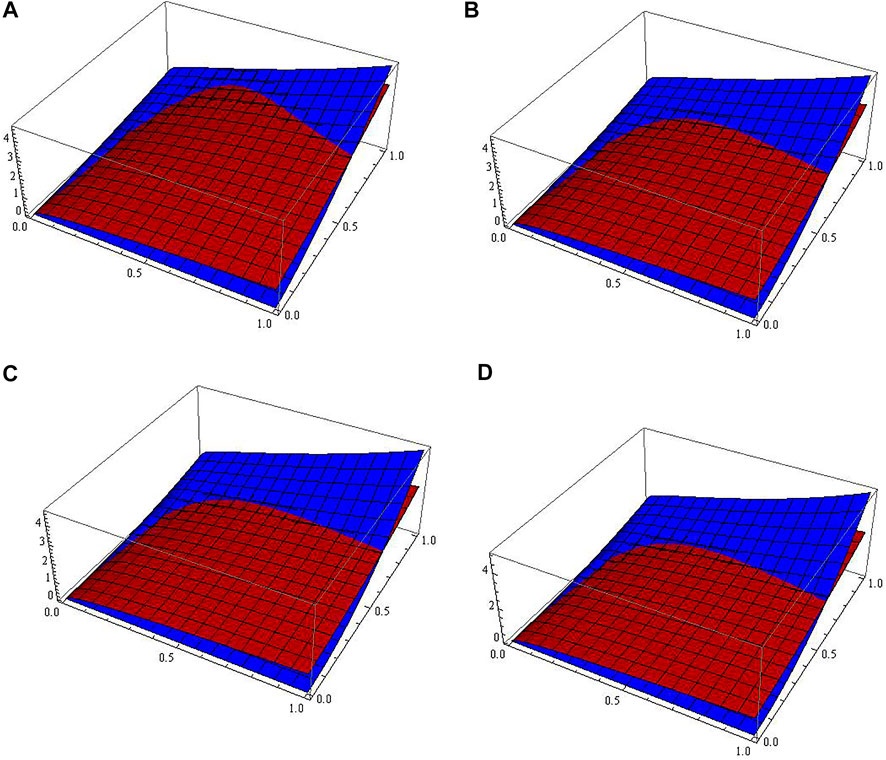
FIGURE 1. Surface graphs of the fifth AS of $U_1\left(x,t\right)$ and $U_2\left(x,t\right)$ in Eq. 81 and the ES of $U_1\left(x,t\right)$ and $U_2\left(x,t\right)$ in Eq. 72 for a fixed value of $\beta =0.5$ and different values of α: (A)$\alpha =0.7$, (B)$\alpha =0.85$, (C)$\alpha =1$, and (D) ES when $\alpha =1$.

Figures 1C,D show that the fifth AS of the IVP (Eq. 70, 71) is excellent compared to the ES, as well as in the previous cases, which have not been documented in order not to increase the numbers of graphs. It is known that, by increasing the number of terms in the series, the accuracy of the solution increases and, thus, the error of solution reduces; therefore, we can reduce the error of the solution by calculating more coefficients of the FME solution as in Eq. 31.

In the next application, the ES is unknown. Therefore, we are trying to find the ES or an appropriate approximation of the solution.

Application 4.4. Consider the following non-homogeneous hyperbolic system of T-FPDEs with variable coefficients:

$U_t^{\left(\alpha \right)}\left(x,t\right)-A\left(x,t\right)U_x^{\left(1\right)}\left(x,t\right)-B\left(x,t\right)U\left(x,t\right)=F\left(x,t\right),0<\alpha \le 1,x\in \mathrm{\Re },t\ge 0,(82)$

subject to

$U\left(x,0\right)=\left(\begin{array}{c}x+1\\ e^x\end{array}\right),(83)$

where

$A\left(x,t\right)=\left(\begin{array}{cc}0& -e^{-x}\left(e^x+\left(x-1\right)E_{\alpha }\left(t^{\alpha }\right)+\left(1+x\right)t^{\alpha }\right)\\ \text{Γ}\left(1+\alpha \right)-e^{x}x-t^{\alpha }x& 0\end{array}\right),$

$B\left(x,t\right)=\left(\begin{array}{cc}{t}^{\alpha }& 1\\ 0& x\end{array}\right),F\left(x,t\right)=\left(\begin{array}{c}x{E}_{\alpha }\left(t^{\alpha }\right)\\ 0\end{array}\right).$

Similar to the previous applications, the LT of Eq. 82 is given by

$\mathbb{U}\left(x,s\right)-\left(\begin{array}{c}x+1\\ e^x\end{array}\right)\frac{1}{s}-\frac{\mathrm{ℒ}\left[{\mathrm{ℒ}}^{-1}\left[\mathbb{A}\left(x,s\right)\right]{\partial }_x^1\left({\mathrm{ℒ}}^{-1}\left[\mathbb{U}\left(x,s\right)\right]\right)\right]}{s^{\alpha }}$

$-\frac{\mathrm{ℒ}\left[{\mathrm{ℒ}}^{-1}\left[\mathbb{B}\left(x,s\right)\right]{\mathrm{ℒ}}^{-1}\left[\mathbb{U}\left(x,s\right)\right]\right]}{s^{\alpha }}-\frac{\mathbb{F}\left(x,t\right)}{s^{\alpha }}=0,0<\alpha \le 1,x\in \mathrm{\Re },s>\lambda \ge 0,(84)$

the kth TS of the expansion of the solution of Eq. 84 is given as

${\mathbb{U}}_k\left(x,s\right)=\left(\begin{array}{c}x+1\\ e^x\end{array}\right)\frac{1}{s}+{\displaystyle \sum _{m=1}^k\frac{H_m\left(x\right)}{s^{1+m\alpha }}},0<\alpha \le 1,x\in \mathrm{\Re },s>\lambda \ge 0,(85)$

and the kth $\text{RMF}$ of Eq. 84 is given by

${\text{RMF}}_k\left(x,s\right)={\mathbb{U}}_k\left(x,s\right)-\left(\begin{array}{c}x+1\\ e^x\end{array}\right)\frac{1}{s}-\frac{\mathrm{ℒ}\left[{\mathrm{ℒ}}^{-1}\left[\mathbb{F}\left(x,s\right)\right]{\partial }_x^1\left({\mathrm{ℒ}}^{-1}\left[{\mathbb{U}}_k\left(x,s\right)\right]\right)\right]}{s^{\alpha }}(86)$

$-\frac{\mathrm{ℒ}\left[{\mathrm{ℒ}}^{-1}\left[\mathbb{B}\left(x,s\right)\right]{\mathrm{ℒ}}^{-1}\left[{\mathbb{U}}_k\left(x,s\right)\right]\right]}{s^{\alpha }}-\frac{\mathbb{F}\left(x,t\right)}{s^{\alpha }},x\in \mathrm{\Re },s>\lambda \ge 0.$

According to the fact in Eq. 37, we can create, successively, the following first eight coefficients of the expansion in Eq. 31 for this application:

$\begin{array}{l}{H}_0\left(x\right)=\left(\begin{array}{c}x+1\\ e^x\end{array}\right),\\ H_1\left(x\right)=\left(\begin{array}{c}1\\ \text{Γ}\left(1+\alpha \right)\end{array}\right),\\ H_2\left(x\right)=\left(\begin{array}{c}1+\text{Γ}\left(1+\alpha \right)\\ 0\end{array}\right),\\ H_3\left(x\right)=\left(\begin{array}{c}1+\frac{\text{Γ}\left(1+2\alpha \right)}{\text{Γ}\left(1+\alpha \right)}\\ 0\end{array}\right),\\ H_4\left(x\right)=\left(\begin{array}{c}1+\frac{\left(1+\text{Γ}\left(1+\alpha \right)\right)\text{Γ}\left(1+3\alpha \right)}{\text{Γ}\left(1+2\alpha \right)}\\ 0\end{array}\right),\\ H_5\left(x\right)=\left(\begin{array}{c}1+\frac{\left(\text{Γ}\left(1+\alpha \right)+\text{Γ}\left(1+2\alpha \right)\right)\text{Γ}\left(1+4\alpha \right)}{\text{Γ}\left(1+\alpha \right)\text{Γ}\left(1+3\alpha \right)}\\ 0\end{array}\right),\\ H_6\left(x\right)=\left(\begin{array}{c}1+\frac{\left(\text{Γ}\left(1+2\alpha \right)+\left(1+\text{Γ}\left(1+\alpha \right)\right)\text{Γ}\left(1+3\alpha \right)\right)\text{Γ}\left(1+5\alpha \right)}{\text{Γ}\left(1+2\alpha \right)\text{Γ}\left(1+4\alpha \right)}\\ 0\end{array}\right),\\ H_7\left(x\right)=\left(\begin{array}{c}1+\frac{\left(\text{Γ}\left(1+\alpha \right)\text{Γ}\left(1+3\alpha \right)+\left(\text{Γ}\left(1+\alpha \right)+\text{Γ}\left(1+2\alpha \right)\right)\text{Γ}\left(1+4\alpha \right)\right)\text{Γ}\left(1+6\alpha \right)}{\text{Γ}\left(1+3\alpha \right)\text{Γ}\left(1+5\alpha \right)}\\ 0\end{array}\right).\end{array}(87)$

Thus, the seventh AS of Eq. 84 has the following expression:

${\mathbb{U}}_7\left(x,s\right)=\frac{H_0\left(x\right)}{s}+\frac{H_1\left(x\right)}{s^{1+\alpha }}+\frac{H_2\left(x\right)}{s^{1+2\alpha }}+\frac{H_3\left(x\right)}{s^{1+3\alpha }}+\frac{H_4\left(x\right)}{s^{1+4\alpha }}+\frac{H_5\left(x\right)}{s^{1+5\alpha }}+\frac{H_6\left(x\right)}{s^{1+6\alpha }}.+\frac{H_7\left(x\right)}{s^{1+7\alpha }},(88)$

so the seventh AS of the IVP (Eqs 82, 83) can be expressed as follows:

$U_7\left(x,t\right)=H_0\left(x\right)+H_1\left(x\right)\frac{t^{\alpha }}{\text{Γ}\left(1+\alpha \right)}+H_2\left(x\right)\frac{t^{2\alpha }}{\text{Γ}\left(1+2\alpha \right)}+H_3\left(x\right)\frac{t^{3\alpha }}{\text{Γ}\left(1+3\alpha \right)}$

$+H_4\left(x\right)\frac{t^{4\alpha }}{\text{Γ}\left(1+4\alpha \right)}+H_5\left(x\right)\frac{t^{5\alpha }}{\text{Γ}\left(1+5\alpha \right)}+H_6\left(x\right)\frac{t^{6\alpha }}{\text{Γ}\left(1+6\alpha \right)}+H_7\left(x\right)\frac{t^{7\alpha }}{\text{Γ}\left(1+7\alpha \right)}.(89)$

To test the AS in Eq. 89, we need to find the norm of residual error vector ($\text{RES}\left(x,t\right)$) for different values of t and x in the region $\left[\mathrm{0,1}]\times [\mathrm{0,1}\right]$, where the residual error vector is defined by

$\begin{array}{c}{\text{RES}}_k\left(x,t\right)\end{array}={\left(U_k\right)}_t^{\left(\alpha \right)}\left(x,t\right)-A\left(x,t\right){\left(U_k\right)}_x^{\left(1\right)}\left(x,t\right)-B\left(x,t\right)U_k\left(x,t\right)-F\left(x,t\right),(90)$

and the Frobenius norm is chosen for error analysis and defined by

$\Vert U\left(x,t\right)\Vert =\sqrt{\left({\displaystyle \sum _{i=1}^m{\displaystyle \sum _{j=1}^n|u_{ij}\left(x,t\right){|}^2}}\right)},U\left(x,t\right)=\left[u_{ij}\left(x,t\right)\right]\in M_{k\times r}.(91)$

Tables 1, 2 show the values of $\left|\left|{\text{RES}}_6\left(x,t\right)\right|\right|$ and $\left|\left|{\text{RES}}_7\left(x,t\right)\right|\right|$, respectively, for different values of α. The data in the tables indicate that the norm of the residual error of the obtained AS decreases as $\left(x,t\right)\to \left(\mathrm{0,0}\right)$ as well as when $\alpha \to 1$. This indicates that the convergence of the BFMTF in Eq. 17 depends on $t,x$, and α as illustrated in Theorem 2.3. As we know, we can reduce the error in the FME solution as we increase the number of terms of the expansion. As we can see from the data in Tables 1, 2, the seventh approximation is more accurate than the sixth approximation. Anyway, it can be said that the L-RPSM is good at providing an accurate AS of a hyperbolic system of T-FPDEs with variable coefficients.

TABLE 1

TABLE 1. Values of $\left|\left|{\text{RES}}_6\left(x,t\right)\right|\right|$ for different values of α.

TABLE 2

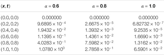
TABLE 2. Values of ${\text{RES}}_7\left(x,t\right)$ for different values of α.

5 Conclusion

We have found that the ES for the hyperbolic system of T-FPDEs with variable coefficients is available if the solution is a linear combination of power functions or if it is a composite of an elementary function and a power function. In case the ES is not available, a good approximation of the solution can be obtained. The L-RPSM is an effective, accurate, easy, and speed technique in obtaining the values of coefficients for the SS. Through this work, we have presented a solution that may be missing for this kind of problem and we have opened the way for researchers to provide other ways to solve this class of equations. Moreover, the newly proposed technique can be used to construct many types of the ordinary or partial DEs of fractional order such as Lane–Emden, Boussinesq, KdV–Burgers, $K\left(m,n\right)$, Klein–Gordon, and $B\left(l,m,n\right)$ equations.

Data Availability Statement

All datasets generated for this study are included in the article/supplementary files.

Author Contributions

The idea of this work, implementation, and output of this form was carried out by both authors.

Conflict of Interest

The authors declare that the research was conducted in the absence of any commercial or financial relationships that could be construed as a potential conflict of interest.

Acknowledgments

The first author expresses his appreciation and thanks to Al-Balqa Applied University for granting him a sabbatical leave that made this research possible.

References

1. Burger M, Caffarelli L, Markowich PA. Partial Differential Equation Models in the Socio-Economic Sciences. Phil Trans R Soc A (2014) 372:20130406. doi:10.1098/rsta.2013.0406

PubMed Abstract | CrossRef Full Text | Google Scholar

2. Mattheij R, Rienstra S, Boonkkamp J. Partial Differential Equations: Modeling, Analysis, Computation, Technische Universiteit Eindhoven Eindhoven. Netherlands: Siam (2005). doi:10.1137/1.9780898718270

CrossRef Full Text

3. Evans LC. Partial Differential Equations. American Mathematical Society (2002). doi:10.1090/gsm/019

4. Leray J. Hyperbolic Differential Equations. Princeton, NJ: Institute for Advanced Study (1953). doi:10.11948/2017095

5. Sanchez Y, Vickers J. Generalised Hyperbolicity in Spacetimes with Lipschitz Regularity. J Math Phys (2017) 58:022502. doi:10.1063/1.4975216

CrossRef Full Text | Google Scholar

6. Toro EF. Notions on Hyperbolic Partial Differential Equations. In: Riemann Solvers and Numerical Methods for Fluid Dynamics. Heidelberg, Berlin: Springer (2009). doi:10.1007/b79761

CrossRef Full Text | Google Scholar

7. Caputo M. Linear Models of Dissipation Whose Q Is Almost Frequency Independent--II. Geophys J Int (1967) 13:529–39. doi:10.1111/j.1365-246x.1967.tb02303.x

CrossRef Full Text | Google Scholar

8. Mainardi F. Fractional Calculus and Waves in Linear Viscoelasticity, Imperial College Press. London, UK: Imperial College (2010). doi:10.1142/p614

CrossRef Full Text

9. Kilbas AA, Srivastava HM, Trujillo JJ. Theory and Applications of Fractional Differential Equations. Netherlands: Elsevier, Amsterdam (2006).

10. Magin RL, Ingo C, Colon-Perez L, Triplett W, Mareci TH. Characterization of Anomalous Diffusion in Porous Biological Tissues Using Fractional Order Derivatives and Entropy. Microporous Mesoporous Mater (2013) 178:39–43. doi:10.1016/j.micromeso.2013.02.054

PubMed Abstract | CrossRef Full Text | Google Scholar

11. Tarasov VE. Fractional Dynamics: Applications of Fractional Calculus to Dynamics of Particles. Fields and Media. Berlin, Germany: Springer (2011).

12. West B, Bologna M, Grigolini P. Physics of Fractal Operators. New York: Springer (2003).

13. Qureshi S, Yusuf A. Mathematical Modeling for the Impacts of Deforestation on Wildlife Species Using Caputo Differential Operator. Chaos, Solitons & Fractals (2019) 126:32–40. doi:10.1016/j.chaos.2019.05.037

CrossRef Full Text | Google Scholar

14. Li Z, Liu Z, Khan MA. Fractional Investigation of Bank Data with Fractal-Fractional Caputo Derivative. Chaos, Solitons & Fractals (2020) 131:109528. doi:10.1016/j.chaos.2019.109528

CrossRef Full Text | Google Scholar

15. Mustapha UT, Qureshi S, Yusuf A, Hincal E. Fractional Modeling for the Spread of Hookworm Infection under Caputo Operator. Chaos, Solitons & Fractals (2020) 137:109878. doi:10.1016/j.chaos.2020.109878

CrossRef Full Text | Google Scholar

16. Ali A, Alshammari FS, Islam S, Khan MA, Ullah S. Modeling and Analysis of the Dynamics of Novel Coronavirus (COVID-19) with Caputo Fractional Derivative. Results Phys (2021) 20:103669. doi:10.1016/j.rinp.2020.103669

PubMed Abstract | CrossRef Full Text | Google Scholar

17. Momani S, Odibat Z. Comparison between the Homotopy Perturbation Method and the Variational Iteration Method for Linear Fractional Partial Differential Equations. Comput Maths Appl (2007) 54:910–9. doi:10.1016/j.camwa.2006.12.037

CrossRef Full Text | Google Scholar

18. Daftardar-Gejji V, Bhalekar S. Solving Multi-Term Linear and Non-linear Diffusion-Wave Equations of Fractional Order by Adomian Decomposition Method. Appl Maths Comput (2008) 202:113–20. doi:10.1016/j.amc.2008.01.027

CrossRef Full Text | Google Scholar

19. Das S, Gupta PK. Homotopy Analysis Method for Solving Fractional Hyperbolic Partial Differential Equations. Int J Comput Maths (2011) 88:578–88. doi:10.1080/00207161003631901

CrossRef Full Text | Google Scholar

20. Momani S, Odibat ZM. Fractional Green Function for Linear Time-Fractional Inhomogeneous Partial Differential Equations in Fluid Mechanics. J Appl Math Comput (2007) 24:167–78. doi:10.1007/bf02832308

CrossRef Full Text | Google Scholar

21. El-Ajou A. Taylor’s Expansion for Fractional Matrix Functions: Theory and Applications. J Math Comput Sci (2020) 21(2):1–17. doi:10.22436/jmcs.021.01.01

CrossRef Full Text | Google Scholar

22. Oqielat Ma. N, El-Ajou A, Al-Zhour Z, Alkhasawneh R, Alrabaiah H. Series Solutions for Nonlinear Time-Fractional Schrödinger Equations: Comparisons between Conformable and Caputo Derivatives. Alexandria Eng J (2020) 59(4):2101–14. doi:10.1016/j.aej.2020.01.023

CrossRef Full Text | Google Scholar

23. El-Ajou A, Oqielat Ma. N, Al-Zhour Z, Momani S. A Class of Linear Non-homogenous Higher Order Matrix Fractional Differential Equations: Analytical Solutions and New Technique. Fract Calc Appl Anal (2020) 23(2):356–77. doi:10.1515/fca-2020-0017

CrossRef Full Text | Google Scholar

24. El-Ajou A, Al-Smadi M, Oqielat Ma. N, Momani S, Hadid S. Smooth Expansion to Solve High-Order Linear Conformable Fractional PDEs via Residual Power Series Method: Applications to Physical and Engineering Equations. Ain Shams Eng J (2020) 11(4):1243–54. doi:10.1016/j.asej.2020.03.016

CrossRef Full Text | Google Scholar

25. El-Ajou A, Oqielat Ma. N, Al-Zhour Z, Momani S. Analytical Numerical Solutions of the Fractional Multi-Pantograph System: Two Attractive Methods and Comparisons. Results Phys (2019) 14:102500. doi:10.1016/j.rinp.2019.102500

CrossRef Full Text | Google Scholar

26. El-Ajou A, Al-Zhour Z, Oqielat Ma., Momani S, Hayat T. Series Solutions of Nonlinear Conformable Fractional KdV-Burgers Equation with Some Applications. Eur Phys J Plus (2019) 134(8):402. doi:10.1140/epjp/i2019-12731-x

CrossRef Full Text | Google Scholar

27. Shqair M, El-Ajou A, Nairat M. Analytical Solution for Multi-Energy Groups of Neutron Diffusion Equations by a Residual Power Series Method. Mathematics (2019) 7(7):633. doi:10.3390/math7070633

CrossRef Full Text | Google Scholar

28. Eriqat T, El-Ajou A, Oqielat Ma. N, Al-Zhour Z, Momani S. A New Attractive Analytic Approach for Solutions of Linear and Nonlinear Neutral Fractional Pantograph Equations. Chaos, Solitons & Fractals (2020) 138:109957. doi:10.1016/j.chaos.2020.109957

CrossRef Full Text | Google Scholar

29. El-Ajou A. Adapting the Laplace Transform to Create Solitary Solutions for the Nonlinear Time-Fractional Dispersive PDEs via a New Approach. Eur Phys J Plus (2021) 136:229. doi:10.1140/epjp/s13360-020-01061-9

CrossRef Full Text | Google Scholar

30. Srivastava VK, Awasthi MK, Tamsir M. RDTM Solution of Caputo Time Fractional-Order Hyperbolic Telegraph Equation. AIP Adv (2013) 3(3):032142. doi:10.1063/1.4799548

CrossRef Full Text | Google Scholar

31. Abbas S, Benchohra M. Fractional Order Partial Hyperbolic Differential Equations Involving Caputo Derivative. Stud Univ Babes-bolyai Math (2012) 57:469–79.

Google Scholar

32. Akilandeeswari A, Balachandran K, Annapoorani N. Solvability of Hyperbolic Fractional Partial Differential Equations. J App Anal Comp (2017) 7:1570–85. doi:10.11948/2017095

Google Scholar

33. Ashyralyev A, Dal F, Pinar Z. On the Numerical Solution of Fractional Hyperbolic Partial Differential Equations. Math Probl Eng (2009) 2009:1–11. doi:10.1155/2009/730465

CrossRef Full Text | Google Scholar

34. Khan H, Shah R, Baleanu D, Kumam P, Arif M. Analytical Solution of Fractional-Order Hyperbolic Telegraph Equation, Using Natural Transform Decomposition Method. Electronics (2019) 8(9):1015. doi:10.3390/electronics8091015

CrossRef Full Text | Google Scholar

35. Modanl M. Two Numerical Methods for Fractional Partial Differential Equation with Nonlocal Boundary Value Problem. Adv Differ Equ (2018) 333:333. doi:10.1186/s13662-018-1789-2

CrossRef Full Text | Google Scholar

36. Lin Y, Xu C. Finite Difference/spectral Approximations for the Time-Fractional Diffusion Equation. J Comput Phys (2007) 225:1533–52. doi:10.1016/j.jcp.2007.02.001

CrossRef Full Text | Google Scholar

37. Meerschaert MM, Tadjeran C. Finite Difference Approximations for Fractional Advection-Dispersion Flow Equations. J Comput Appl Maths (2004) 172:65–77. doi:10.1016/j.cam.2004.01.033

CrossRef Full Text | Google Scholar

38. Kochubei AN. Fractional-hyperbolic Systems. Fract Calc Appl Anal (2013) 16:860–73. doi:10.2478/s13540-013-0053-4

CrossRef Full Text | Google Scholar

39. Hendy AS, Macías-Díaz JE, Serna-Reyes AJ. On the Solution of Hyperbolic Two-Dimensional Fractional Systems via Discrete Variational Schemes of High Order of Accuracy. J Comput Appl Maths (2019) 354:612–22. doi:10.1016/j.cam.2018.10.059

CrossRef Full Text | Google Scholar

40. Simon T. Mittag-Leffler Functions and Complete Monotonicity. Integral Transforms Special Fun (2015) 26 (1):36–50. doi:10.1080/10652469.2014.965704

CrossRef Full Text | Google Scholar