Static Schwinger-Level Electric Field Nonlinearities and Their Significance to Photons and Photon Entanglement

In this work, we postulate that Schwinger’s threshold for a dynamic electric field intensity to induce spatial nonlinearity is a special case and, more generally, it is the threshold field for both static and dynamic electric fields. Fields of this magnitude induce negative-energy charges to adapt positive energy attributes; within an atom, they also support interstate energy transfers and intrastate chaotic mixing of time-varying fields. Nonlinearity-induced chaos forms the basis for the probabilistic nature of photon creation. Answers to physical problems at atomic and lower scales continuously evolve because chaotic-like electron movements change their configurations on a time scale of 10 zs. Within atoms, frequency mixing that creates an optical frequency field occurs in the nonlinear region surrounding the nucleus. On a probabilistic basis, a ring of vacuum charge can be induced that forms into an equivalent waveguide, which confines the energy as it travels permanently away from the atom. The propagating relativistically augmented fields losslessly induce charges that bind and protect the energy-carrying fields. The photon charge-field ensemble is a closed system and possesses all first-order photon properties, including zero rest mass and permanent stability. For near-neighbor photons traveling at a speed approaching c, we find a small constant force between them that is dependent upon their relative spin orientations. Our model shows that the radius of a photon is ≈10 am and that photon wavelength information is coded by energy.

Introduction

Photon properties are of ongoing scientific interest [1–14], with commercial applications that include optical communication [15–17], temporal imaging [18–20], and supercontinuum generation [21–23]. It has been noted [24] that the amount of information carried by a photon is potentially enormous, and utilizing this information would enable quantum communication systems with extraordinary capacities and exceptional levels of security [25, 26]. This work presents a unique photon model that details structure, propagation, and spontaneous generation. It is an interdisciplinary study of atomic and optical phenomena based upon techniques selected from physics, electrical engineering, and optics. We present our ideas, conclusions, and thoughts that led us to them with the hope it will assist others with their research and development.

Schwinger calculated that a dynamic electromagnetic field of 1.3 × 10¹⁸ V/m is the threshold between which the vacuum of space presents low-field linear and high-field nonlinear responses [27]. To foster a complete understanding of this effect, many capable experimentalists have attempted to create a Schwinger threshold field in the laboratory using lasers [28–38] but have been unsuccessful. They explain the difficulty as nonlinearity-induced charge transitions and resulting unavoidable effects that extract energy. This leaves characteristics of high-intensity fields as a largely unexplored regime.

Moderate-intensity physical phenomena such as waves and particle interactions at a distance are linear phenomena and well understood on the basis of superposition with other linear phenomena, but the superposition principle cannot be used to construct particles. For example, nonlinearities are essential for the creation of a lepton pair from a high-energy photon. The desire to understand particle formation has resulted in many and extensive studies to determine the results of adding nonlinear terms to known linear equations but without widespread success. Although Schwinger’s threshold field, as derived, applies only to dynamic electromagnetic fields, we postulate that it is a special case of the general rule that threshold-level electromagnetic fields, static and dynamic, force a nonlinear response from the spatial vacuum that shifts negative-energy charges to positive energies and thus prevent any field, including static ones, from exceeding his calculated threshold value. We then apply conventional linear physics to determine results and report them in this article.

Jackson [39] pointed out that static nuclear fields near atomic nuclei are as large as 10²¹ V/m. Indeed, regions with a calculated Coulomb field exceeding the threshold field are ubiquitous and centered on every atomic nucleus. In many cases, the nonlinear region extends to distances of 150 fm and Schrödinger’s equation shows that a portion of every atomic eigenstate lies within that region. Since atomic emission satisfies the Manley–Rowe equations [40] and since they are trivial in linear media, we take the agreement as evidence of nonlinearity in atoms. Since each eigenstate contains a nonlinear volume and since eigenstate electrons are dynamic entities, we anticipate that chaotic-like behavior of electrons is subject only to the constraints of atomic conservation laws.

Combining the idea of charge induction from vacuum with the theory of waveguides provides a means of creating an ordered, hybrid charge—electromagnetic field structure that exhibits first-order properties of photons, including permanent stability. Since photon construction requires a confluence of events, its completion is probabilistic; however, with satisfactory conditions, a ring of charge proportional to cosϕ, centered on the axis of propagation, is induced that supports and guides the electromagnetic fields. With propagation, the ring of charge extends, with the leading edge of the fields, becoming a circular cylinder that supports an energy packet that is both closed and stable. Only the photon energy propagates; charges are induced in position by the fields, retained in position as they bind and guide the passing fields, and losslessly return to negative-energy states after photon passage. From the calculated photon size, it appears that photon wavelength information is coded by energy.

Herein, the model we present shows that both classical electromagnetism and a disruption of the local three-dimensional spatial continuum are essential for a photon’s existence. Our results show the photon is intrinsically both a wave and a particle [41–52], wherein the ‘particle’ is charge-induced by the fields of the photon, which exceed the Schwinger nonlinearity threshold, from the Dirac vacuum. It is the only model we are aware of that explains an ultrashort monochromatic pulse: a photon.

In the “Fields and Charges of an Atom” section, we discuss the chaotic nature of the fields and charges within an atom. In the “A One-Dimensional Pulse” section, we discuss a stable, closed charge-field ensemble with known first-order photon properties. Then, the “Photon Construction and Emission” section discusses spontaneous emission, induced emission, and photon size. In the “Photon Entanglement” section, we examine the force between two near-neighbor photons propagating in the same direction identical in all respects except in one case where the spins have the same direction and in another case the spins have opposite directions. For each case, we find that there is a small force between them: the force is time-varying with parallel spins and attractive with antiparallel spins.

Fields and Charges of an Atom

With c representing the speed of light, ℏ the reduced Planck’s constant, and m and e electron mass and charge, the threshold field is as follows [27]:

$E_S=m^2{c}^3/e\hslash \simeq 1.3\times {10}^{18}{\text{Vm}}^{-1}.(1)$

Several laser groups report attempts to create Schwinger’s threshold field in the laboratory, but without success. The difficulty is that, in accordance with Dirac’s theory, the fields force electron-positron pairs to tunnel to positive energies, separate them into independent existences, and then accelerate them in opposite directions. These actions extract the transformation energy and leave the science of extreme electric fields relatively unexplored [28–38]. In the absence of experimental information, we postulate that both static and dynamic fields force charge transformation from negative to positive energies. With static fields, instead of a dynamic reaction, the opposite surface charge density is retained in equilibrium positions between the repulsive creating field and attractive fields of their own making. Dittrich and Gies point to an equivalence between properties of dielectric media and quantum vacuum properties, with the Lamb shift and the Casimir effect as evidence [53, 54]. Virtual pairs in vacuum and actual pairs in polarized media respond to applied fields similarly and, in some cases, the virtual pairs may include milli-charges [55–58]. Although event details near the threshold field intensity have not been explored, naturally occurring static fields of this magnitude occur in the immediate vicinity of all atomic nuclei [39]. An internal atomic nonlinearity creates power-frequency transitions in accordance with the Manley–Rowe relationships [40]; we take its occurrence as evidence that Schwinger’s nonlinearity extends to static nuclear fields.

Table 1 lists relevant nuclear parameters and associated fields for six selected elements. The second column is atomic number Z; the third column is nuclear radius R_N, calculated using the formula R_N = 1.07A^1/3, where A is the number of contained nucleons; the fourth column shows the calculated nuclear surface-to-threshold field ratio, with E_N denoting the nuclear field at the surface of the nucleus; the fifth column shows radius R_S, at which the field, calculated using nuclear charge and Coulomb’s law, drops to the threshold value.

TABLE 1

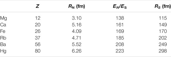
TABLE 1. Relevant nuclear parameters for bare atomic nuclei.

For atoms with a full complement of electrons and, with r representing the radius, the actual value of R_S is less than that shown in Table 1 because of time-average electron charge at r < R_S; accuracy may be increased by including electron charge within the Schwinger region, R_N < r < R_S, particularly as calculated using descriptive Schrödinger wave functions as corrected [59, 60].

From the perspective of classical physics, Schrödinger’s equation is based upon a Fourier integral transform between spatial and momentum spaces, and such transforms are valid if and only if both spaces are linear and at least piecewise continuous. Therefore, the equation is and is not valid, respectively, within linear and nonlinear spaces, and the behaviors of charges and fields in the nonlinear medium are both unknown and unknowable. Within the nonlinear region, we know only that the static field intensity equals E_S and charge density exists throughout the region, but have no knowledge of the detailed ebb and flow of charge under the influence of added fields. Atomic radii are on the order of 100 pm and R_S sizes are on the order of 200 fm. Although the nonlinearity occupies about 10⁻⁸ of an atom’s interior space, we suggest it has a major influence on atomic interactions since only it is subject to chaotic mixing [61–63]. In the linear region, charge is distributed throughout the eigenstates in a manner that conserves time and space averages of energy, linear momentum, and angular momentum as the charge distributions cycle through all possible formations. The intrinsic electron frequency and wavelength are ν₀ = mc²/h = 7.8 × 10²⁰ Hz and λ = h/mc = 386 fm; hence, charge configurations are perturbed at the rate of about 7.8 ×10²⁰ per second. An electron has no known components or substructure; we take the simplified view of an electron as an adaptive charged cloud that maintains said parameters. When free of constraints, the electron becomes a sphere of charge, and within an eigenstate, it expands to occupy the entire state in accordance with the wave function. As illustrated in Supplementary Material SI-1, interactions within the nonlinear region, in a small but continuous way, supply sufficient chaotic energy into each eigenstate to keep nonconserved atomic properties aperiodic.

The Manley–Rowe power-frequency relationships govern the rate at which intra-atomic nonlinearities create interfrequency energy exchanges [40]. We briefly remind the reader, since the relationships are critical to what follows, that during an interaction between the electrons of two eigenstates, with different energies and frequencies, either up- or downconversion may occur, but only with a concurrent energy transfer at their difference frequency. For example, with P₁ and ω₁ and P₂ and ω₂ representing, respectively, initial and final eigenstate powers and frequencies and P and ω representing the generated radiation, the Manley–Rowe equations are as follows:

$\frac{P_1}{{\omega }_1}+\frac{P_2}{{\omega }_2}=0\text{and}\frac{P_1}{{\omega }_1}-\frac{P}{\omega }=0.(2)$

These equations govern lossless oscillating systems; by convention, power emission is positive. A time integral shows the energy-to-frequency ratio is constant between interacting systems.

The Nonlinear Region

By the postulated extension of Schwinger’s results to static fields, threshold field E_S for the onset of spatial nonlinearity applies to the static fields created by atomic nuclei. Retaining the field value at E_S can only be accomplished by a negative charge layer about the nucleus and a positive charge density distributed throughout the full nonlinear region. By the divergence theorem and with κ denoting charge density, ^ a unit vector, ε₀ the permittivity of free space, and r the radial distance from the center of the nucleus, the charge density is $\kappa =\nabla \cdot \left({\epsilon }_0{E}_S\widehat{r}\right)=2{\epsilon }_0{E}_S/r$. The resulting charge density and total induced positive charge are as follows:

$\begin{array}{l}\kappa =2{\epsilon }_0{E}_S/r,\\ q_0=Ze\left(1-R_N^2/R_S^2\right).\end{array}(3)$

Since ± charges are induced in equal measure, the magnitude of the negative charge adjacent to the nucleus is –q₀. An additional field applied to the region would not affect the field magnitude, but it would affect κ(r); as we shall show, this idea appears key to radiation emission by atoms.

A One-Dimensional Pulse

An antenna cannot create a field with a large wavelength-to-size ratio that propagates outward in less than three dimensions, yet photons certainly lie within that wavelength-to-size ratio and propagate in one dimension. Microwave techniques use waveguides to obtain one-dimensional propagation, yet empty space contains no obvious means to construct one. We construct a working model of a photon that is based upon and consistent with classical electromagnetism, supports one-dimensional waves, and accurately describes first-order properties of optical photons. Both experimental and quantum theoretical studies have investigated possible photon structures [64–71]. Quite differently from them, we utilize steady-state solutions of the electromagnetic equations to examine how one-dimensional flows of microwave fields are created and controlled and then seek to determine if an atom could use a similar but scaled technique to generate and control optical radiation. In this section, we detail the fields and associated layers of induced charge on the surface of a one-dimensional, circularly cylindrical dielectric waveguide of radius b.

Only for TEM modes does the speed of propagation approach c; all other propagation modes are significantly slower. Another characteristic of all modes, except TEM waveguide modes, is the longest possible propagating wavelength. Looking ahead to the results shown in “Photon Size Estimates” section, our calculated photon radius is so small, at frequencies of interest, that neither TE or TM modes will propagate. Therefore, we consider only TEM modes.

Electric potential Φ satisfies the wave equation ∇²Φ – ∂²Φ /∂t² = 0, with k the separation constant between space and time solutions, propagation in the z-direction obeys ∂²Φ /∂z² + k²Φ = 0, and the time and space dependence is $e^{i\left(\omega t-kz\right)}$, where ω is the radian frequency and k is the wavenumber. The potential in the transverse plane satisfies the Laplacian equation, to which, using cylindrical coordinates (ρ, ϕ, z), the solutions are potentials $\Phi =\rho e^{-j\varphi }\text{and}{e}^{-j\varphi }/\rho$; we are concerned with both. Both i and j = ±(−1)^1/2, with i being associated with space-time and j the azimuth angle.

With boldface indicating vector, the full set of fields, both internal and external, guided by a thin dielectric tube of radius b is as follows:

$\begin{array}{l}{\mathit{E}}_{in}={\mathit{E}}_0\left(\widehat{\rho }-j\widehat{\varphi }\right)e^{-j\varphi }{e}^{i\left(\omega t-kz\right)}:c{\mathit{B}}_{in}=j{\mathit{E}}_{in}\\ {\mathit{E}}_{ex}=-{\mathit{E}}_0\frac{b^2}{{\rho }^2}\left(\widehat{\rho }+j\widehat{\varphi }\right)e^{-j\varphi }{e}^{i\left(\omega t-kz\right)}:c{\mathit{B}}_{ex}=-j{\mathit{E}}_{ex}\end{array}(4)$

With Eq. 4, the equality j = 0 or j = ±i yields, respectively, linearly or circularly polarized fields. The flux lines for ρ < b are straight lines and for ρ > b form a circular arc.

With interior and exterior fields present, the charge density κ, current density I, and fields within the interface at radius b are as follows:

$\begin{array}{l}{\mathit{E}}_b=-j{E}_0\widehat{\varphi }{e}^{-j\varphi }{e}^{i\left(\omega t-kz\right)}c{\mathit{B}}_b=j{E}_0\widehat{\rho }{e}^{-j\varphi }{e}^{i\left(\omega t-kz\right)}\\ \kappa =2{\epsilon }_0{E}_0{e}^{-j\varphi }{e}^{i\left(\omega t-kz\right)}\eta \mathit{I}=2E_0\widehat{z}{e}^{-j\varphi }{e}^{i\left(\omega t-kz\right)}\end{array}(5)$

Figure 1 depicts both inner and outer field forms and interfacial charge density κ. The charge and current densities are essential for the system to function; its value is determined by the difference in electric field intensities across the interface as the wave propagates; although individual charges remain in situ, the magnitudes and phases propagate and satisfy Eq. 5. In the reference frame of the waveguide, although the actual z-directed charge motion is zero, current Eq. 5 is created by wave propagation past charge density κ at speed c.

FIGURE 1

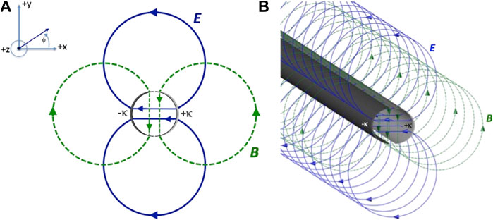
FIGURE 1. (A) A plot of Eq. 4 that illustrates a transverse section of the fields. The center ring represents the waveguide, and the right and left semicircular arcs represent, respectively, layers of positive and negative polarization charges described by Eq. 5. Solid lines represent electric flux, and dotted lines represent magnetic flux. The interior flux lines are straight and intercept the guide wall at angle ϕ₀, where –π/2 < ϕ₀ < π/2. The exterior flux lines are circular, centered at y = csc(ϕ₀)/2, normal to the guide wall and, if continued through it, would pass through the axis. All electric flux lines stop and start on polarization charges and all magnetic flux lines surround z-directed effective polarization currents (not shown). (B) A plot of the same equation showing an extended length of waveguide.

With circular polarization, the Poynting vector N, field energy W, and linear momentum M_z, supported by length l of the tube, are as follows:

$\begin{array}{l}{\mathit{N}}_{in}=\widehat{z}{E}_0^2/\eta :W=\pi \epsilon E_0^2{b}^{2}l:M_z=W/c{\mathit{N}}_{ex}=\widehat{z}\frac{E_0^2}{\eta }\frac{b^4}{{\rho }^4}:W=\pi \epsilon E_0^2{b}^{2}l:M_z=W/c\end{array}(6)$

With the gauge in which the fields are functions of only the vector potential, $A_{\varphi }=E_{\varphi }/i\omega$, where $E_{\varphi }$ is that of Eq. 5. With asterisk representing complex conjugate, the linear momentum per unit length equals product Aκ*/2. The angular momentum L about the z-axis is equal to the line integral of radius b times Aκ*/2:

$L=-2\widehat{z}\frac{ij}{\omega }\pi {\epsilon }_0{E}_0^2{b}^{2}l=-ij\frac{W}{\omega }\widehat{z}.(7)$

Retaining only the real part of Eq. 7 with respect to j or writing j = ± i, the energy-to-angular momentum ratios are, respectively, W/L = ∞ or W/L = ± ω. The linear and angular momenta result, respectively, from the field-flux product and the field-charge product.

The full interfacial boundary conditions are equal magnitude, antiparallel field components $E_{\rho }$ and $B_{\varphi }$ and equal magnitude, parallel field components $E_{\varphi }$ and $B_{\rho }$. The fields of Eq. 4 satisfy these conditions and the uniqueness theorem assures that the coaxial field ensemble described above uniquely possesses these properties: no other field forms can meet the same constraints. The external fields extend outward and mix with the environment but remain attached to the originating charges.

Regarding the different interior and exterior field forms, the energy of the inner and outer forms are singular, respectively, at infinity and zero. This requires separate solutions for the inner and outer regions of space, connected through matched boundary conditions. Both inner and outer fields are TEM modes, but only the inner field is a section of a plane wave. The initial magnitude of photon radius b is determined by the unknown separation distance between semicircular layers of positive- and negative-induced charges, as seen in Figure 1, charge-induced and separated by the static Schwinger-level field. Between the layers of induced charge, a counterelectric field is formed of equal magnitude and it induces charges as the pulse propagates. Were b to enlarge, the electric field magnitude would decrease, new charges could not be induced, and the beam would cease to exist; hence, it exists as a 1D structure.

The Photon as a Closed System

Volume integrals of the field-flux and source-potential products yield, respectively, the total field energy and the field energy that remain attached to the source. Each of the four integrals of Eq. 8, two field-flux and two source-potential integrals, has the value $W=\pi \epsilon E_0^2{b}^{2}l$. Field-flux integrals are evaluated over all space and include both free-standing flux and flux that remains attached to its source. The source-potential integrals are evaluated over space occupied by the sources and thus include only flux that remains attached to its source. Equality of the two forms shows that there are no free-standing flux lines: all flux remains permanently attached to its source. Therefore, a photon is a separate and closed system. As illustrated in Figure 1, all electric flux lines remain attached to source charges and all magnetic flux lines encircle source currents. The following energy relationships apply:

$\begin{array}{c}\frac{{\epsilon }_0}{4}{\displaystyle \int \mathit{E}\cdot {\mathit{E}}^{\ast }dV}=\frac{1}{4}{\displaystyle \int \Phi {\kappa }^{\ast }dV}=\pi {\epsilon }_0{E}_0^2{b}^{2}l\\ \frac{1}{4{\mu }_0}{\displaystyle \int \mathit{B}\cdot {\mathit{B}}^{\ast }dV}=\frac{1}{4}{\displaystyle \int \mathit{A}\cdot {\mathit{J}}^{\ast }dV}=\pi {\epsilon }_0{E}_0^2{b}^{2}l\end{array}.(8)$

By Thomson’s theorem, an isolated field ensemble cannot be stable [72]. Does the theorem extend to the above pulse and its accompanying charges? Let µ₀ represent the permeability of free space and assign a positive or negative sign, respectively, to repulsive or compressive pressures; the surface pressure Γ_s from substituting the fields of Eq. 4 into the electromagnetic stress tensor and with circular polarization is as follows:Γ

${\Gamma }_S=\left({\epsilon }_0{E}^2-B^2/{\mu }_0\right)/4=0.(9)$

There is no net pressure at any point on the interfacial surface: the pulse is stable. Additional energy is required to change either the radius or the direction of the pulse. As such, the ensemble is a closed, stable entity.

Speed of Propagation

The underlying postulate of the special theory of relativity is that the idealized speed of light c is the same in all reference frames, with the corollary that every structure is subject to its laws. However, considerable work has shown that not all light structures travel at speed c [1–9]. Our model indicates that a photon can exist in the described form only if the entire edifice of charges and fields created by the waveforms of Eqs. 4, 5 propagate as a unit. Consider waveform Eq. 5 as it propagates within the induced charge density that defines the interface. The charges create a small but actual positive relative permittivity. In response, a portion of separation constant k moves from the z-dependent wave equation, thereby decreasing the z-directed speed, to the transverse portion, thereby introducing z-dependence into the two-dimensional array of fields, leaving Figure 1B as an approximation to the actual result and the propagation speed of the entire edifice at u < c.

Elapsed time and length in the direction of motion differ from values measured in the moving frame by the Lorentz contraction, Λ:

$\mathit{\Lambda }=\underset{u\to c}{\lim }{\left(1-u^2/c^2\right)}^{-1/2}.(10)$

Electromagnetic fields are also affected. With primes indicating a fixed reference frame, electromagnetic fields in the stationary frame that are normal to the motional velocity in terms of those in the moving frame are as follows:

$\begin{array}{l}{\mathit{E}}^{\prime }=\mathit{\Lambda }\left(\mathit{E}-\mathit{u}\times \mathit{B}\right),\\ {\mathit{B}}^{\prime }=\mathit{\Lambda }\left(\mathit{B}+\mathit{u}\times \mathit{E}/c^2\right).\end{array}(11)$

Combining Eq. 11 with Eq. 4 shows that the effective fields in the stationary frame are produced by fields in the moving frame as it passes by at speed u are as follows:

$\begin{array}{l}{\mathit{E}}_{in}=2\mathit{\Lambda }{\mathit{E}}_0\left(\widehat{\rho }-j\widehat{\varphi }\right)e^{-j\varphi }{e}^{i\left(\omega t-kz\right)}:c{\mathit{B}}_{in}=j{\mathit{E}}_{in}\\ {\mathit{E}}_{ex}=-2\mathit{\Lambda }{\mathit{E}}_0\frac{b^2}{{\rho }^2}\left(\widehat{\rho }+j\widehat{\varphi }\right)e^{-j\varphi }{e}^{i\left(\omega t-kz\right)}:c{\mathit{B}}_{ex}=-j{\mathit{E}}_{ex}\end{array}(12)$

For the special case of the virtual waveguide, since the fields are normal to the direction of propagation, the magnitudes are 2Λ greater than otherwise.

Photon Construction and Emission

The competing interpretations of semiclassical and quantum theories of optics are nowhere starker than with spontaneous emission [73, 74]. As previously discussed, the Manley–Rowe equations, and more generally the nonlinear nature of oscillators [75], indicate electromagnetic field generation occurs within the nonlinear region of the atom. That region is spherical with a radius ∼30 times greater than the nucleus itself, while the radius of the complete atom is ∼10⁴ times greater than that of the nonlinear region; see Table 1. To exit an atom, radiation must first traverse the linear region of the atom with its plasma-like cloud of charge.

Why Atoms Do Not Behave Like Antennas

The Q of any radiating object is commonly defined as Q = ωW_pk/P_av, where W_pk is the peak standing energy of the radiation field, and P_av is the time average output power. With all antenna radiation the least possible value is that of a dipole field, for which Q ≈ 1/(ka)³ [76, 77], with k = 2π/λ and a the radius of a virtual sphere just enclosing the antenna. With atoms emitting at optical wavelengths, ka is ≈10⁻³ and hence Q ≈ 10⁹. For something the size of an atom radiating optical wavelengths, the reactive, or standing, energy would be ≈ 10⁹ greater than the output power per cycle. However, while an antenna is a fixed system, often a metallic conductor, and is restricted in its ability to respond to an applied source, an atom is an adaptive system with no such physical constraints and responds to local force fields. Adaptive systems minimize energy and minimization of standing energy dictates the total absence of radiated power.

Consider an atom with two eigenstates between which selection rules permit energy exchanges: high-energy eigenstate one is occupied and low-energy eigenstate two is not. The high-energy electron supports frequency ω₁, as seen in Eq. 2, and the low-energy electron is capable of supporting frequency ω₂. When both states, or a portion of both states, are in the nonlinear region difference, frequency ω is created; the energy is either emitted or reflected back to the source electron. Emission from an atom requires the field to move into and through the linear region, radius ∼100 fm to ∼100 pm, with its adaptable electron charge.

With ε representing permittivity, after the field enters the linear region, the dipole field has the following form:

$E=\frac{p}{4\pi \epsilon r^3}\left\{2\sin \theta \widehat{r}-\left(\cos \theta \widehat{\theta }\pm j\widehat{\varphi }\right)\right\}{e}^{\pm j\varphi }{e}^{i\left(\omega t-kr\right)}.(13)$

The electron-cloud responds to any and all entering fields by generating an electric dipole field that is identical in all respects except magnitude and phase: the newly formed field is π out-of-phase with the incoming field and reflects the applied energy back to the source. The same process applies to any and all higher-order multipole fields [78]. Supplementary Material SI-2 presents a third approach to understanding why such fields are not observed.

Moore penned a reconstructed conversation between Bohr and Schrödinger, in which Schrödinger explained the type of signal he would expect during ‘quantum jumps,’ and the signals should be large enough to be detected outside the atom, but they are not [79]. The above procedure describes the extinguishing process applicable to all waveforms that interact with the atom’s complement of electrons, hence the absence of ‘quantum jump’ radiation.

Photon Construction by an Atom

Critical photon-creation events necessarily occur during a time period not exceeding the time for a propagating field to exit the atom, ∼10⁻¹⁹ s; hence, a complete mathematical description includes transient solutions of the electromagnetic equations, and they are not available. Therefore, by default, our analysis is based upon a steady-state description of the optical frequency radiation that first enters linear space and the contained pulse as it traverses the atom’s linearly responding, electron-filled region.

The many mutual characteristics of circular dielectric waveguides and photons are discussed in “A One-Dimensional Pulse” section and lead us to closely examine if natural processes expected within atoms can create an equivalent waveguide. An important theorem of classical electromagnetics applicable to linear media is that the source of every electromagnetic field may be expressed as a sum over its own unique set of multipolar fields. At optical frequencies, the ka ratio of atoms, and more so the nuclear region, is so small that only the dipole terms are meaningful and of them only the first expansion term provides a significant output, and that requires order and degree modal numbers (1, ±1) [78].

By our model, for optical radiation to exit the atom, the three-dimensional expanse of the dipole field generated by the transition of energy from one eigenstate to another must compress into a TEM mode propagating within a one-dimensional waveguide that protects it from outside influences as it traverses the electronic portion of the atom and, without reflection, exits into free space. It has no rest mass, it propagates at speed approaching c, and it is stable.

Optical selection rules require the photon to carry angular momentum; this, in turn, requires rotating dipole moments p that are described by both.

$\mathit{p}=p\left(\widehat{x}\mp i\widehat{y}\right)e^{i\omega t}=p\left(\widehat{\rho }\mp i\widehat{\varphi }\right)e^{i\left(\omega t\mp \varphi \right)}.(14)$

The circularly polarized electric dipole fields that uniquely result from these requirements, written with scalar value of p, are:

$\mathit{E}=\frac{p}{4\pi \epsilon r^3}\left\{2\sin \theta \widehat{r}-\left(\cos \theta \widehat{\theta }\mp i\widehat{\varphi }\right)\right\}{e}^{i\left(\omega t-kr\mp \varphi \right)}.(15)$

We next consider if field Eq. 15 can generate a waveguide-like structure of charge with radius b that binds and guides the fields. For that purpose, it is convenient to reexpress it using a mix of spherical (r, θ, ϕ) and (ρ, ϕ, z) cylindrical coordinates. Including the static nuclear field E_N, our choice for describing the total electric fields is the mixed coordinate forms:

$\mathit{E}=\frac{p}{4\pi \epsilon r^3}\left\{3\sin \theta \widehat{r}-\left(\widehat{\rho }\mp i\widehat{\varphi }\right)\right\}{e}^{i\left(\omega t-kr\mp \varphi \right)}+E_N\widehat{r}.(16)$

To detail the analysis, we choose an optical wavelength of 500 nm (frequency ν = 600 THz, period τ = 1.7 fs). Since propagation time for light to traverse the linear region is about ∼10⁻¹⁹ s, approximately 10⁴ times less than the period of the wave, for this analysis, we consider the dipole field to be static. We consider Eq. 16 immediately after it is formed at radius r differentially greater than R_S, and hence E_N ≅ E_S. Since our only source of a charge density that could serve as a cylindrical waveguide is through the divergence of an electric field, we note, after defining E₀ = −p/4πεr³, that the actual dipole field of Eq. 16 on and near the z-axis is as follows:

$\mathit{E}=E_0\left[\widehat{\rho }\cos \left(\omega t-kz\mp \varphi \right)+\widehat{\varphi }\sin \left(\omega t-kz\mp \varphi \right)\right].(17)$

We anticipate the magnitude of E₀ to be less than but comparable to E_N; see Supplementary Material SI-2. The total field magnitude on and near the z-axis is (E₀² + E_N²)^1/2 > E_S and large enough to induce charge density:

$\kappa ={\epsilon }_0{E}_0\cos \left(\omega t-kz\mp \varphi \right).(18)$

Inspection of Eq. 17 at field points radius b and angular positions ϕ and π + ϕ shows the field symmetry is

${\mathit{E}}_0\left(b\right)={\mathit{E}}_0\left(-b\right).(19)$

The field has even parity. Next, consider the static nuclear field at the same field points. Field vectors to each point from the z-axis have the following symmetry:

${\mathit{E}}_{\mathrm{N}}\left(b\right)=-{\mathit{E}}_{\mathrm{N}}\left(-b\right).(20)$

The field has odd parity.

At r differentially greater than R_S, Eq. 19 shows that construction of an appropriate charge-waveguide wall requires even parity; however, Eq. 20 shows the nuclear field, required to obtain a total field in excess of the threshold field, has odd parity. With θ₀ being the angle from the origin (centered on the nucleus) to points b, a suitable wave-guiding charge density can be formed by satisfying the following inequality:

$\left|E_0\cos \left(\omega t-k{R}_S-\varphi \right)\right|>>E_{\mathrm{N}}\sin {\theta }_0.(21)$

Conditions for charge induction are sinθ₀ < E₀ /E_N and a wave phase angle small enough so $\cos \left(\omega t-k{R}_S\mp \varphi \right)$ is ≈ one. Since $E_N\sin \theta$ vanishes on the z-axis, there must be a value of b for which the inequality is satisfied. Charge is induced within the disk of radius b, which becomes a ring of charge density proportional to cosϕ via the process described in “The Nonlinear Region” section.

Formation of the ring of charge changes the fields from three-dimensional to one-dimensional with a significant difference in boundary conditions. Matching the altered boundary conditions changes the fields to that of Eq. 22:

$\mathit{E}=E_0\left(\widehat{\rho }\mp i\widehat{\varphi }\right)e^{i\left(\omega t-kz\mp \varphi \right)}:c\mathit{B}=i\mathit{E}.(22)$

The stage is set for photon propagation.

The initial charge induction was enabled by static field E_N, and E_N decreases by 1/r² and therefore effective for only a relatively small distance from the nucleus. In its place, with a propagation speed approaching c, the relativistically augmented magnitude of E₀ equals or exceeds E_S, as seen in Eq. 12, and it forces charge induction. Since the waveguide-cylinder is lossless and hence retains all field energy, E₀ is constant. The fields of Eq. 22 have the exact form of Eq. 4 and satisfy the requirement of zero divergence throughout the region. At radius b, the induced charge density is that of Eq. 18 and the surface current density is

$\eta \mathit{I}=\widehat{z}{\mathit{E}}_0\cos \left(\omega t-kz\mp \varphi \right).(23)$

Together, Eq. 18 and Eq. 23 describe surface effects on a circular, dielectric waveguide of radius b that isolates interior fields from exterior influences. For this reason, and unlike all other fields, this specific edifice of field and charge does not suffer the fate discussed in “Why Atoms Do Not Behave Like Antennas” section but propagates through the linear, electron-containing portion of the atom and, without incident, propagates outward into free space. The photon continues to induce charges as it propagates. It also rotates once each field cycle and, by doing so, creates alternating bands of positive and negative charge that form into a double helix.

Since the surface charge densities created by the internal and external TEM fields of Eq. 4 are superimposed, the charge densities create either or both fields. Creating both conserves photon energy and momentum and decreases the interfacial induced charge density by a factor of √2, but it also leaves open their relative magnitudes. For example, is the energy equally divided between regions, or does it oscillate back and forth between them?

To summarize, although subject to chaotic disturbances, the field of a propagating wave must be generated by two eigenstates at least partially within the nonlinear region and endure long enough to complete the transition. After the field has been created, it must retain an appropriate form until all available energy transfers into the linear region. After entering the linear region, propagation requires the initial formation of the ring of charge by fields E₀ and E_N and the subsequent onset of the magnetic and electric fields arising from the modified boundary conditions. The magnitude of E₀, when appropriately modified by relativistic considerations, must be large enough so that when propagating at a speed approaching c, induced charges will be continuously formed. The cumulative effect of these uncertainties is that the onset of spontaneous emission is probabilistic.

As per the known absence of linearly polarized photons, linearly polarized dipole fields do not induce an enclosing, field-protecting charge structure and hence cannot propagate in accordance with the discussion of “Why Atoms Do Not Behave Like Antennas” section.

Photon Size Estimates

As noted in “Speed of Propagation” section, a photon propagates at speed less than c; the exact value is unknown, yet photon characteristics depend upon it. Photon parameters of interest are the electric field intensity E₀, radius b, l the photon length in its own reference frame, and the fractional wavelength l/λ. The energy-size relationship is shown in Eq. 6, given by $W=\pi {\epsilon }_0{E}_0^2{b}^{2}l=h\nu /2$.

Continued induction of the photon-enclosing cylindrical charge array requires that ΛΕ₀ = E_S and, as discussed in “Speed of Propagation” section, the speed of propagation approaches c. It is convenient to introduce new variable, speed ratio α, where

$u/c=\left(1-{10}^{-\alpha }\right):\Lambda \cong {10}^{\alpha /2}/\sqrt{2}.(24)$

The dipole field intensity is

$E_0=\sqrt{2}{E}_S\times {10}^{-\alpha /2}.(25)$

These equations are adequate to construct Table 2.

TABLE 2

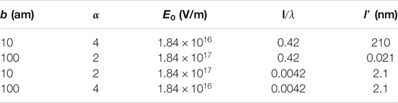
TABLE 2. Relationships between photon parameters and size.

Column one is photon radius b in attometers, column two is speed ratio α, column three is field intensity E₀ calculated from Eq. 25, column four is ratio of photon length l determined in its own reference frame to wavelength for λ = 500 nm, and column five is the photon length observed as the photon passes. Nature’s means of coding information about photon frequency bears on acceptable photon sizes. For example, if coding is by energy, the ratio $l/\lambda =0.0042$ may be acceptable, but if coding is by wavelength, a ratio of at least $l/\lambda =0.42$ must surely be required. Given these numbers, we believe that photon wavelength information is coded by energy: λ = hc/E.

We note that the interior of an atom will be shielded from an incident EM plane wave by the surrounding electron charge distribution. However, in regard to our photon model, specifically the estimated sizes shown in Table 2, we find the photon is accurately viewed as a needle. The energy of the needle-like photon is localized, resulting in an immense energy density. Consequently, the charge density surrounding an atom does not materially interfere with photon absorption.

Stimulated Emission and Absorption

Since we have no transient solutions of the electromagnetic equations, we can only outline a few parameters that will surely be significant for the process. By our model of an atom, the activating photon must penetrate the nonlinear region to incite an energy exchange; it is there that all energy exchanges occur. Therefore, the photon must penetrate the atomic volume and traverse inwardly through the linear region. The ratio of the linear-to-nonlinear radii, 100 pm to 100 fm, is about 1,000; as an example, iron has an estimated nuclear radius of 4,000 am and, by Table 2, photon radius b is in the 10–100 am range. It is ‘needle-like’ even on a nuclear scale of dimensions. We postulate that the small size and high-energy density of the photon enable it to penetrate the atom without degradation. Since there is no time delay between the probabilistic onset of incoming radiation and a stimulated output, we conclude there are no time-delaying probabilistic events required to complete the exchange, such as those required for spontaneous emission, from which we conclude the incoming photon acts as an enabling template for its daughter photon.

Photon Entanglement

Since two photons described by a single wave function occur most frequently with near-neighbors, we use our photon model to calculate the transverse force between a pair of neighboring photons propagating along parallel paths. If interphoton forces do not adjust the charge structures, we show that a small attractive force is created between pairs with antiparallel spins, and a sinusoidally time-varying force is created between pairs with parallel spins.

As noted in “Photon Construction by an Atom” section with atomic values of ka, only the lowest-order term in an expansion for the dipole field needs to be retained [78]. Our concern here is any force that may exist between near-neighbor photons propagating on parallel paths that are identical in all respects except the spins may be either parallel or antiparallel. Step-by-step details are given in Supplementary Material SI-3.

Defining χ = ωt – kz, our concern is the outer phasor fields of Eq. 4 which implicitly travel at speed c:

$\mathit{E}={\mathit{E}}_0\frac{b^2}{{\rho }^2}\left(-\widehat{x}\pm i\widehat{y}\right)e^{i\left(\chi \pm 2\varphi \right)}:c\mathit{B}={\mathit{E}}_0\frac{b^2}{{\rho }^2}\left(\mp i\widehat{x}-\widehat{y}\right)e^{i\left(\chi \pm 2\varphi \right)}.(26)$

We can calculate the force most directly by using the actual parts of the fields:

$\begin{array}{l}\mathit{E}={\mathit{E}}_0\frac{b^2}{{\rho }^2}\left[-\widehat{x}\cos \left(\chi \pm 2\varphi \right)\mp \widehat{y}\sin \left(\chi \pm 2\varphi \right)\right],\\ c\mathit{B}={\mathit{E}}_0\frac{b^2}{{\rho }^2}\left[\pm \widehat{x}\sin \left(\chi \pm 2\varphi \right)-\widehat{y}\cos \left(\chi \pm 2\varphi \right)\right].\end{array}(27)$

Re‐expressing Eq. 27 using trigonometric functions of single variables gives the following:

$\begin{array}{l}\mathit{E}=E_0\frac{b^2}{{\rho }^2}\left[\widehat{x}\langle -\cos 2\varphi \cos \chi \pm \sin 2\varphi \sin \chi \rangle -\widehat{y}\langle \pm \cos 2\varphi \sin \chi +\sin 2\varphi \cos \chi \rangle \right],\\ c\mathit{B}=E_0\frac{b^2}{{\rho }^2}\left[\widehat{x}\langle \pm \cos 2\varphi \sin \chi +\sin 2\varphi \cos \chi \rangle +\widehat{y}\langle -\cos 2\varphi \cos \chi \pm \sin 2\varphi \sin \chi \rangle \right].\end{array}(28)$

We seek the force between two near-neighbor photons that are identical in all respects, with the two photons having either parallel or antiparallel spins. They propagate in the +z-direction and are spaced Δx = 2d between centers. Consider a virtual planar strip yΔz through x = 0 that extends between y = ±∞. The fields expressed in Eq. 28 are those of a photon at (-d,y). The photon located at position (+d,y) creates the fields of Eq. 29:

$\begin{array}{l}\mathit{E}=E_0\frac{b^2}{{\rho }^2}\left(\widehat{x}\langle -\cos 2\varphi \cos \chi \mp \sin 2\varphi \sin \chi \rangle -\widehat{y}\langle \pm \cos 2\varphi \sin \chi -\sin 2\varphi \cos \chi \rangle \right),\\ c\mathit{B}=E_0\frac{b^2}{{\rho }^2}\left(\widehat{x}\langle \pm \cos 2\varphi \sin \chi -\sin 2\varphi \cos \chi \rangle +\widehat{y}\langle -\cos 2\varphi \cos \chi \mp \sin 2\varphi \sin \chi \rangle \right).\end{array}(29)$

For photons with parallel spins, the summed fields on the strip are as follows:

$\begin{array}{l}{\mathit{E}}_{\uparrow \uparrow }=E_0\frac{2b^2}{{\rho }^2}\left(-\widehat{x}\cos 2\varphi \cos \chi \mp \widehat{y}\cos 2\varphi \sin \chi \right),\\ c{\mathit{B}}_{\uparrow \uparrow }=E_0\frac{b^2}{{\rho }^2}\left(\pm \widehat{x}\cos 2\varphi \sin \chi -\widehat{y}\cos 2\varphi \cos \chi \right).\end{array}(30)$

For photons with antiparallel spins, the summed fields on the strip are as follows:

$\begin{array}{l}{\mathit{E}}_{\uparrow \downarrow }=-\widehat{x}{E}_0\frac{2b^2}{{\rho }^2}\left(\pm \cos 2\varphi \cos \chi +\sin 2\varphi \sin \chi \right),\\ c{\mathit{B}}_{\uparrow \downarrow }=-\widehat{y}{E}_0\frac{2b^2}{{\rho }^2}\left(\cos 2\varphi \cos \chi \pm \sin 2\varphi \sin \chi \right).\end{array}(31)$

The electromagnetic stress tensor shows the separation pressure at each point on the strip is proportional to the square of the y-directed field component minus the square of the x-directed field component. Inspection shows that, in both cases, there is no field pressure and hence no force between adjacent photons. So long as the spacing satisfies the inequality d > b, photons may be packed together arbitrarily closely. This is consistent with the Bose-Einstein condition that unlimited numbers of photons may be packed into a single quantum state.

However, the conclusion of no force between the photons is correct only for photons traveling at speed c and, as discussed in “Speed of Propagation” and “Photon Construction by an Atom” sections, u < c. For a more precise determination of the forces, we replace c with u in field terms Eqs. 30, 31. Substituting Eq. 24 into Eq. 30 and Eq. 31 and solving for the pressure shows

$\begin{array}{l}{P}_{\uparrow \uparrow }=4\epsilon b^4{E}_0^2·{10}^{-\alpha }{\left(\frac{y^2-d^2}{{\rho }^4}\right)}^2\cos 2\chi ,\\ P_{\uparrow \downarrow }\cong -4\epsilon b^4{E}_0^2·{10}^{-\alpha }\left\{{\left(\frac{y^2-d^2}{{\rho }^4}\right)}^2{\cos }^2\chi \pm \frac{2}{{\rho }^4}\left(\frac{2dy}{{\rho }^2}\right)\left(\frac{d^2-y^2}{{\rho }^2}\right)\sin \chi \cos \chi +{\left(\frac{2dy}{{\rho }^4}\right)}^2{\sin }^2\chi \right\}.\end{array}(32)$

Integrating over the entire strip shows that there are small but significant forces in the two cases:

$\begin{array}{l}{F}_{\uparrow \uparrow }=-\pi \epsilon \left(\Delta z\right)\frac{b^4}{d^3}{E}_0^2\cdot {10}^{-\alpha }\cos 2\chi ,\\ F_{\uparrow \downarrow }=-\pi \epsilon \left(\Delta z\right)\frac{b^4}{d^3}{E}_0^2\cdot {10}^{-\alpha }.\end{array}(33)$

The residual forces between photons with identical wave numbers are small and, as shown in Eq. 33, between both parallel and antiparallel photon pairs have equal magnitudes. However, the force between photons with parallel spins is sinusoidally time-varying and, since the magnitude decreases with increasing distance, separation increases with each pulse until they become independent entities. Since the force between photons with antiparallel spins is constant and attractive, they remain as a unit until or unless separated by an external force. We suggest the described forces between near-neighbor photons provide a classical physics basis to help understand photon entanglement [11–14], otherwise considered to be a purely quantum effect.

The guiding and confining charges lie in an intermediate range between positive and negative energies, not entirely in either, and hence remain attached to Dirac’s negative-energy sea of charge, and there is no known speed limitation for signals between negative-energy states.

Conclusions and Discusssion

The key points of this work are based upon the postulate that both static and dynamic [27], threshold-level electromagnetic fields force a nonlinear response from the spatial vacuum that induces negative-energy charges to adapt positive energy characteristics and thus prevent any field from exceeding the threshold value. Jackson noted static nuclear fields should be as large as 10²¹ V/m [39]. This postulate enables us to model an atom’s nuclear region as a positive nucleus surrounded by a concentric nonlinear region of radius R_S, with an induced nucleus-adjoining layer of negative charge. An equal amount of induced positive charge is arrayed between R_S and the negative charge layer; at all points E = E_S and the vacuum within responds nonlinearly to applied fields.

With spontaneous emission, the filled high-energy and the empty low-energy states can only exchange energy when parts of both are in the nonlinear region in accordance with the Manley–Rowe equations [40]. Optical frequency energy is created and located in the immediate vicinity of the nucleus. Our view of photon formation and emission by the atom is discussed in “Photon Construction and Emission” section; it requires that linear space supports high-intensity electromagnetic waves and that nonlinear space induces the layers of charge that guide the waves. After emission, arrays of field-induced vacuum charge form an equivalent optical waveguide that guides and confines the energy as it travels endlessly away from the atom. All participating charge remains in situ: none propagates and hence there is no rest mass. During propagation, fields at the pulse front, enlarged by Lorentz relativistic contraction, continuously induce in situ arrays of positive energy, charged pairs, and the charges remain in position during pulse passage, after which they losslessly drop back to the negative-energy state.

The monochromatic charge-field photon ensemble described herein, in “A One-Dimensional Pulse” section, propagates at a speed approaching c and possesses the following unique properties: {1} the propagating ensemble has no unbalanced charge and no rest mass; {2} energy-to-linear momentum ratio is c; {3} energy-to-angular momentum ratio is ω. The waveguide is a z-directed circular cylinder of an induced charge layer proportional to cosϕ. With propagation, the cylinder rotates once each field cycle, by which the bands of positive and negative charge form a double helix. The photon structure permits the calculation of the force between neighboring photons, separately calculated for parallel and antiparallel spins. The pair with parallel spins suffers a small sinusoidal force that increases the separation with each cycle. The pair with antiparallel spins is subject to a constant attractive force that entangles the pair unless disturbed by outside forces.

Only nonlinearities can create the deviations from equilibrium that constitute an electromagnetic particle. The photon particle is a closed entity consisting of TEM waves propagating past a pair of induced ± arrays of vacuum charge that confines and guides the propagation. The uniqueness theorem assures that only the fields described by Eq. 4 support a photon’s full assortment of electromagnetic and kinematic photon properties. The energies of potential-charge and field-flux products are equal and shown in Eqs. 8 and 9 and require that all fields possess the static property of remaining attached to their sources.

Knowledge of chaos, chaos-like activity, the Schwinger threshold field, the Dirac vacuum, and the details of constraints on radiation by electrically small antennas were not available when Einstein wrote that only nonlinear field equations can create the deviations from equilibrium that constitute an electromagnetic particle [80]. The arrays of charged pairs induced by Schwinger’s vacuum nonlinearity enable the function Einstein described when he wrote to Sommerfeld in 1909 of the ‘ordering of the energy of light around discrete points that move with the velocity of light’ [81]. As our work shows, the photon is comprised of fields of sufficient magnitude to induce charges that, in turn, guide and bind the fields. In 1917 Einstein [82] noted that spontaneous emission is probabilistic in nature, leaving the time and direction of the process to chance. In this work the uncertainties lie between Eq. 16 through Eq. 21, with the photon created if and only if the system satisfies all criteria.

With our analysis, it is not quantum mechanics that underlies chaos but chaos that underlies quantum mechanics. Free electrons pulsate at frequency ω = mc²/ħ; with trapped electrons, the frequency is decreased by atomic binding energies. Within linear media, the response to such cycles is repetitive and readily predictable, as seen in Supplementary Material SI-1, but within nonlinear media, the response continually varies and is probabilistic. Experimental measurements of atomic systems yield probabilistic responses; it follows that measurements yield exact answers at the moment the measurement is taken. During the process of taking a series of measurements, the atomic electrons continuously evolve, influenced by properties of both linear and nonlinear regions, and yield exact but different answers at each time slot: a summation of all such readouts is probabilistic.

Our ability to describe photon creation and emission using classical physics suggests that statistical analysis based upon the chaotically induced motion of its parts underlies quantum mechanics. After a sufficient time and an extended number of pulses, solutions become chaotic attractors. They are also the probabilistic answers that result from Schrödinger’s equation; since any two things equal to the same thing are equal to each other, it follows that solutions of Schrödinger’s equation are chaotic attractors.

Data Availability Statement

The original contributions presented in the study are included in the article/Supplementary Material; further inquiries can be directed to the corresponding author.

Author Contributions

DG and CG both derived the mathematical equations presented in this work, analyzed the inherent physical concepts, and cowrote the manuscript.

Conflict of Interest

The authors declare that the research was conducted in the absence of any commercial or financial relationships that could be construed as a potential conflict of interest.

Acknowledgments

The authors gratefully acknowledge the help of Monica Claire Flores of Daegu Gyeongbuk Institute of Science and Technology (DGIST) with the figures. CG acknowledges early-stage support of this work by the Air Force Office of Scientific Research, Contract F49620-96-1-0353.

Supplementary Material

The Supplementary Material for this article can be found online at: https://www.frontiersin.org/articles/10.3389/fphy.2020.590531/full#supplementary-material.

References

1. Giovannini D, Romero J, Potoček V, Ferenczi G, Speirits F, Barnett SM, et al. Optics. Spatially structured photons that travel in free space slower than the speed of light. Science (2016) 347:857–60. doi:10.1126/science.aaa3035

CrossRef Full Text | Google Scholar

2. Saari P. Reexamination of group velocities of structured light pulses. Phys Rev A (2018) 97:063824. doi:10.1103/physreva.97.063824

CrossRef Full Text | Google Scholar

3. Alfano RR, Nolan DA. Slowing of Bessel light beam group velocity. Optic Commun (2016) 361:25–7. doi:10.1016/j.optcom.2016.12.079

CrossRef Full Text | Google Scholar

4. Bouchard F, Harris J, Mand H, Boyd RW, Karimi E. Observation of subluminal twisted light in vacuum. Optica (2016) 3:351–4. doi:10.1109/pn.2015.7292539

CrossRef Full Text | Google Scholar

5. Zhou ZY, Nolan DA, Vaziri A, Weihs G, Zeilinger A. Quantum twisted double-slits experiments: confirming wavefunctions’ physical reality. Sci Bull (2017) 62:1185–92. doi:10.1364/nlo.2017.nw3b.5

CrossRef Full Text | Google Scholar

6. Fedorov MV, Vintskevich SV. Diverging light pulses in vacuum: Lorentz-invariant mass and mean propagation speed. Laser Phys (2017) 27:036202. doi:10.1088/1555-6611/aa567f

CrossRef Full Text | Google Scholar

7. Petrov NI. Speed of structured light pulses in free space. Sci Rep (2019) 9:18332. doi:10.1038/s41598-019-54921-5

PubMed Abstract | CrossRef Full Text | Google Scholar

8. Lyons A. How fast is a twisted photon?. Optica (2018) 5:682–6.

CrossRef Full Text | Google Scholar

9. Vintskevich SV, Grigoriev DA. Structured light pulses and their Lorentz-invariant mass. Laser Phys (2019) 29:086001. doi:10.1088/1555-6611/ab1aa0

CrossRef Full Text | Google Scholar

10. Ojima I, Saigo H. Photon localization revisited. Mathematics (2015) 3:897–912. doi:10.3390/math3030897

CrossRef Full Text | Google Scholar

11. Stute A. Tunable ion-photon entanglement in an optical cavity. Nature (2012) 485:482–5. doi:10.1038/nature11120

PubMed Abstract | CrossRef Full Text | Google Scholar

12. BlattCasabone JM, Brune M, Haroche S. Manipulating quantum entanglement with atoms and photons in a cavity. Rev Mod Phys (2001) 73:565–82.

CrossRef Full Text | Google Scholar

13. Togan E. Quantum entanglement between an optical photon and a solid-state spin qubit. Nature (2010) 466:730–4. doi:10.1038/nature09256

PubMed Abstract | CrossRef Full Text | Google Scholar

14. LukinChu A, Vaziri A, Weihs G, Zeilinger A. Entanglement of the orbital angular momentum states of photons. Nature (2001) 412:313–6. doi:10.1038/35085529

PubMed Abstract | CrossRef Full Text | Google Scholar

15. Yan QR, Li ZH, Hong Z, Zhan T, Wang YH. Photon-counting underwater wireless optical communication by recovering clock and data from discrete single photon pulses. IEEE Photonics J (2019) 11:7905815. doi:10.1109/jphot.2019.2936833

CrossRef Full Text | Google Scholar

16. Bashir MS, Alouini MS. Signal acquisition with photon-counting detector arrays in free-space optical communications. IEEE Trans Wireless Commun (2020) 19:2181–95. doi:10.36227/techrxiv.11435847

CrossRef Full Text | Google Scholar

17. Paterson C. Atmospheric turbulence and orbital angular momentum of single photons for optical communication. Phys Rev Lett (2005) 94:153901. doi:10.1103/PhysRevLett.94.153901

PubMed Abstract | CrossRef Full Text | Google Scholar

18. Mazelanik M, Leszczynski A, Lipka M, Parniak M. Temporal imaging for ultra-narrowband few-photon states of light. Optica (2020) 7:203–8. doi:10.1364/optica.382891

CrossRef Full Text | Google Scholar

19. Denis S, Moreau PA, Devaux F, Lantz E. Temporal ghost imaging with twin photons. J Optic (2017) 19:034002. doi:10.1088/2040-8986/aa587b

CrossRef Full Text | Google Scholar

20. Ding Y, Aguilar AC, Li CQ. Axial scanning with pulse shaping in temporal focusing two-photon microscopy for fast three-dimensional imaging. Optic Express (2017) 25:33379–88. doi:10.1364/oe.25.033379

CrossRef Full Text | Google Scholar

21. Zhao Y. Two-photon microscope using a fiber-based approach for supercontinuum generation and light delivery to a small-footprint optical head. Opt Lett (2020) 45:909–12. doi:10.1364/OL.381571

PubMed Abstract | CrossRef Full Text | Google Scholar

22. Iftimia A, Baker C, El Amraoul M, Messaddeq Y. Broadband supercontinuum generation in As₂Se₃ chalcogenide wires by avoiding the two-photon absorption effects. Optic Lett (2013) 38:1185–7. doi:10.1364/ol.38.001185

CrossRef Full Text | Google Scholar

23. Weigand R, Wittmann M, Guerra JM. Generation of femtosecond pulses by two-photon pumping supercontinuum-seeded collinear traveling wave amplification in a dye solution. Appl Phys B (2001) 73:201–3. doi:10.1007/s003400100632

CrossRef Full Text | Google Scholar

24. Malik M, Erhard M, Huber M, Krenn M, Fickler R, Zeilinger A. Multi-photon entanglement in high dimensions. Nat Photon (2016) 10:248–52. doi:10.1364/fio.2016.fw3f.1

CrossRef Full Text | Google Scholar

25. Cerf NJ, Bourennane M, Karlsson A, Gisin N. Security of quantum key distribution using d-level systems. Phys Rev Lett (2002) 88:127902. doi:10.1103/PhysRevLett.88.127902

PubMed Abstract | CrossRef Full Text | Google Scholar

26. Mirhosseini M. High-dimensional quantum cryptography with twisted light. New J Phys (2015) 17:033033. doi:10.1364/qim.2019.s2a.3

CrossRef Full Text | Google Scholar

27. Schwinger J. On gauge invariance and vacuum polarization. Phys Rev (1951) 82:664–79.

CrossRef Full Text | Google Scholar

28. Hubbell JH. Electron–positron pair production by photons: a historical overview. Radiat Phys Chem (2006) 75:614–23. doi:10.1016/j.radphyschem.2005.10.008

CrossRef Full Text | Google Scholar

29. Dunne GV. New strong-field QED effects at extreme light infrastructure, nonperturbative vacuum pair production. Eur Phys J D (2009) 55:327–40. doi:10.1140/epjd/e2009-00022-0

CrossRef Full Text | Google Scholar

30. Monin A, Voloshin MB. Semiclassical calculation of photon-stimulated Schwinger pair creation. Phys Rev D (2010) 81:085014. doi:10.1103/physrevd.81.085014

CrossRef Full Text | Google Scholar

31. Borisov AB, McCorkindale JC, Poopalasingam S, Longworth JW, Rhodes CK. Reaching vacuum harmonic generation and approaching the Schwinger limit with X-rays. Contrib Plasma Phys (2013) 53:179–86. doi:10.1002/ctpp.201310031

CrossRef Full Text | Google Scholar

32. Bulanov SS, Esirkepov TZ, Thomas AG, Koga JK, Bulanov SV. Schwinger limit attainability with extreme power lasers. Phys Rev Lett (2010) 105:220407. doi:10.1103/PhysRevLett.105.220407

PubMed Abstract | CrossRef Full Text | Google Scholar

33. Blaschke D, Gevorgyan NT, Panferov AD, Smolyansky SA. Schwinger effect at modern laser facilities. J Phys Conf (2016) 672:012020. doi:10.1088/1742-6596/672/1/012020

CrossRef Full Text | Google Scholar

34. Schneider C, Schutzhold R. Prefactor in the dynamically assisted Sauter–Schwinger effect. Phys Rev D (2016) 94:085015. doi:10.1103/physrevd.94.085015

CrossRef Full Text | Google Scholar

35. Aleksandrov IA, Plunien G, Shabaev VM. Pulse shape effects on the electron-positron pair production in strong laser fields. Phys Rev D (2017) 95:056013. doi:10.1103/physrevd.95.056013

CrossRef Full Text | Google Scholar

36. Anton W, Bauke H, Keitel CH. Multi-pair states in electron–positron pair creation. Phys Lett B (2016) 760:552–7. doi:10.1016/j.physletb.2016.07.037

CrossRef Full Text | Google Scholar

37. Panferov AD, Smolyansky SA, Otto A, Kämpfer B, Blaschke DB, Juchnowski L. Assisted dynamical Schwinger effect: pair production in a pulsed bifrequent field. Eur Phys J D (2016) 70:56. doi:10.1140/epjd/e2016-60517-y

CrossRef Full Text | Google Scholar

38. Meuren S, Keitel CH, Di Piazza A. Semiclassical picture for electron–positron photoproduction in strong laser fields. Phys Rev D (2016) 93:085028. doi:10.1103/physrevd.93.085028

CrossRef Full Text | Google Scholar

39. Jackson JD Classical electrodynamics. 3rd ed. New York: John Wiley (1999).

CrossRef Full Text | Google Scholar

40. Manley JM, Rowe HE. General energy relations in nonlinear reactances. Proc IRE (1950) 47:2115–6.

CrossRef Full Text | Google Scholar

41. Aharonov Y, Zubairy MS. Time and the quantum: erasing the past and impacting the future. Science (2005) 307:875–9. doi:10.1126/science.1107787

PubMed Abstract | CrossRef Full Text | Google Scholar

42. Baldzuhn J, Mohler E, Martienssen W. A wave–particle delayed-choice experiment with a single-photon state. Z Phys B (1989) 77:347–52.

CrossRef Full Text | Google Scholar

43. Lawson-Daku BJ. Delayed choices in atom Stern–Gerlach interferometry. Phys Rev A (1996) 54:5042–7. doi:10.1103/physreva.54.5042

PubMed Abstract | CrossRef Full Text | Google Scholar

44. BaudonAsimov YH. Delayed “Choice” quantum eraser. Phys Rev Lett (2000) 84:1–5. doi:10.1103/PhysRevLett.84.1

PubMed Abstract | CrossRef Full Text | Google Scholar

45. ScullyYu V. Experimental realization of Wheeler's delayed-choice gedanken experiment. Science (2007) 315:966–8. doi:10.1126/science.1136303

PubMed Abstract | CrossRef Full Text | Google Scholar

46. RochWu V. Delayed-choice test of quantum complementarity with interfering single photons. Phys Rev Lett (2008) 100:220402. doi:10.1103/PhysRevLett.100.220402

PubMed Abstract | CrossRef Full Text | Google Scholar

47. RochWu R, Terno DR. Proposal for a quantum delayed-choice experiment. Phys Rev Lett (2011) 107:230406. doi:10.1103/PhysRevLett.107.230406

PubMed Abstract | CrossRef Full Text | Google Scholar

48. Ma X. Experimental delayed-choice entanglement swapping. Nat Phys (2012) 8:479–84. doi:10.1038/nphys2294

CrossRef Full Text | Google Scholar

49. Ma XS. Quantum erasure with causally disconnected choice. Proc Natl Acad Sci USA (2013) 110:1221–6. doi:10.1073/pnas.1213201110

PubMed Abstract | CrossRef Full Text | Google Scholar

50. ZeilingerKofler JS. Realization of quantum Wheeler’s delayed-choice experiment. Nat Photon (2012) 6:600–4. doi:10.1109/cleoe-iqec.2007.4386903

CrossRef Full Text | Google Scholar

51. Tang JS. Revisiting Bohr’s principle of complementarity using a quantum device. Phys Rev A (2013) 88:014103. doi:10.1103/physreva.88.014103

CrossRef Full Text | Google Scholar

52. Danan A. Asking photons where they have been. Phys Rev Lett (2013) 111:240402. doi:10.1103/PhysRevLett.111.240402

PubMed Abstract | CrossRef Full Text | Google Scholar

53. VaidmanFarfurnik W, Gies H. Light propagation in nontrivial QED vacua. Phys Rev D (1998) 58:025004.

CrossRef Full Text | Google Scholar

54. Dittrich W, Gies H. Probing the quantum vacuum. Berlin: Springer-Verlag (2000).

CrossRef Full Text | Google Scholar

55. Gies H, Jaeckel J, Ringwald A. Polarized light propagating in a magnetic field as a probe for millicharged fermions. Phys Rev Lett (2006) 97:140402. doi:10.1103/PhysRevLett.97.140402

PubMed Abstract | CrossRef Full Text | Google Scholar

56. Melchiorri A, Polosa AD, Strumia A. New bounds on millicharged particles from cosmology. (2007). May 23, 2007. arXiv:hep-ph/0703144v2.

CrossRef Full Text | Google Scholar

57. Diamond M, Schuster P. Searching for light dark matter with the SLAC millicharge experiment. Phys Rev Lett (2013) 111:221803. doi:10.1103/PhysRevLett.111.221803

PubMed Abstract | CrossRef Full Text | Google Scholar

58. Liu Z, Zhang Y. Probing millicharges at BESIII via monophoton searches. Phys Rev D (2019) 99:015004.

CrossRef Full Text | Google Scholar

59. Hartree DR. The calculation of atomic structures. New York: John Wiley (1957).

CrossRef Full Text | Google Scholar

60. Slater JC. Quantum theory of atomic structure. New York: McGraw-Hill (1960).

CrossRef Full Text | Google Scholar

61. Bishop R. In: E. N. Zalta, editor. Chaos, (Spring 2017 Edition). The Stanford Encyclopedia of Philosophy (2017).

CrossRef Full Text | Google Scholar

62. Berry M. Quantum chaology, not quantum chaos. Phys Scripta (1989) 40:335–6.

CrossRef Full Text | Google Scholar

63. Berry M. The bakerian lecture, 1987: quantum chaology. Proc Roy Soc Lond A (1987) 413:183–98.

CrossRef Full Text | Google Scholar

64. Duke DW, Owens JF. Photon structure-function as calculated using perturbative quantum chromodynamics. Phys Rev D (1980) 22:2280–5.

CrossRef Full Text | Google Scholar

65. Scott DM, Stirling WJ. Longitudinal structure-function of the photon in super-symmetric quantum chromodynamics. Phys Rev D (1984) 29:157–8.

CrossRef Full Text | Google Scholar

66. Glück M, Reya E, Vogt A. Parton structure of the photon beyond the leading order. Phys Rev D (1992) 45:3986–94.

CrossRef Full Text | Google Scholar

67. Nisius R, Seymour MH. QED structure functions of the photon. Phys Lett B (1999) 452:409–13.

CrossRef Full Text | Google Scholar

68. Nisius R. The Photon Structure from deep inelastic electron-photon scattering. Phys Rep (2000) 332:165–317.

CrossRef Full Text | Google Scholar

69. Krawczyk M, Zembrzuski A, Staszel M. Survey of the present data on photon structure functions and resolved photon processes. Phys Rep (2001) 345:266–450. doi:10.1016/s0370-1573(00)00105-8

CrossRef Full Text | Google Scholar

70.The ZEUS Collaboration. Dijet photoproduction at HERA and the structure of the photon. Eur Phys J C (2002) 23:615–31. doi:10.1063/1.1402837

CrossRef Full Text | Google Scholar

71. Krupa B, Lesiak T, Pawlik B, Wojton T, Zawiejaki L. The study of the photon structure functions in the ILC energy range. Acta Phys Polonica B (2015) 46:1329–36. doi:10.5506/aphyspolb.46.1329

CrossRef Full Text | Google Scholar

72. Bakhoum EG. Proof of Thomson’s theorem of electrostatics. J Electrost (2008) 66:561–3. doi:10.1016/j.elstat.2008.06.002

CrossRef Full Text | Google Scholar

73. Milonni PW. Semiclassical and quantum-electrodynamical approaches in nonrelativistic radiation theory. Phys Rep (1976) 25:1–81.

CrossRef Full Text | Google Scholar

74. Milonni PW. Different ways of looking at the electromagnetic vacuum. Phys Scripta (1988) T21:102–9.

CrossRef Full Text | Google Scholar

75. Armstrong EH. Some recent developments of regenerative circuits. Proc IRE (1922) 10:244–60.

CrossRef Full Text | Google Scholar

76. McLean JS. A re-examination of the fundamental limits on the radiation Q of electrically small antennas. IEEE Trans Antenn Propag (1996) 44:672–6.

CrossRef Full Text | Google Scholar

77. Grimes DM, Grimes CA. Radiation Q of dipole generated fields. Radio Sci (1999) 34:281–96.

CrossRef Full Text | Google Scholar

78. Panofsky WKH, Phillips M. Classical electricity and magnetism. 2nd ed. Boston, MA: Addison-Wesley Publishing Co. (1962). p. 11–4.

CrossRef Full Text | Google Scholar

79. Moore W. Schrödinger life and thought. Cambridge: Cambridge University Press (1998). p. 200–22.

CrossRef Full Text | Google Scholar

80. Schilpp PA. Albert Einstein: philosopher-scientist. New York City, New York: MJF Books (1970). p. 89.

CrossRef Full Text | Google Scholar

81. Pais A. Letter to A. Sommerfeld, September 29, 1909, The Life and Science of Albert Einstein. Oxford: Oxford Press (1982), p. 403.

CrossRef Full Text | Google Scholar

82. Einstein A. The Quantum theory of Radiation. Phys. Z. (1917), 18: 121–128.

CrossRef Full Text | Google Scholar