 Raunak Dey
 Subhrokoli Ghosh
 Avijit Kundu
 Ayan Banerjee
94% of researchers rate our articles as excellent or good
Learn more about the work of our research integrity team to safeguard the quality of each article we publish.
Find out more
ORIGINAL RESEARCH article
Front. Phys. , 15 January 2021
Sec. Optics and Photonics
Volume 8 - 2020 | https://doi.org/10.3389/fphy.2020.576948
This article is part of the Research Topic Optical Trapping (Laser Tweezers) and Nanosurgery (Laser Scissors) View all 31 articles
True random number generators are in high demand for secure cryptographic algorithms. Unlike algorithmically generated pseudo-random numbers they are unclonable and non-deterministic. A particle following Brownian dynamics as a result of the stochastic Ornstein-Uhlenbeck process is a source of true randomness because the collisions with the ambient molecules are probabilistic in nature. In this paper, we trap colloidal particles in water using optical tweezers and record its confined Brownian motion in real-time. Using a segment of the initial incoming data we train our learning algorithm to measure the values of the trap stiffness and diffusion coefficient and later use those parameters to extract the “white” noise term in the Langevin equation. The random noise is temporally delta correlated, with a flat spectrum. We use these properties in an inverse problem of trap-calibration to extract trap stiffnesses, compare it with standard equipartition of energy technique, and show it to scale linearly with the power of the trapping laser. Interestingly, we get the best random number sequence for the best calibration. We test the random number sequence, which we have obtained, using standard tests of randomness and observe the randomness to improve with increasing sampling frequencies. This method can be extended to the trap-calibration for colloidal particles confined in complex fluids, or active particles in simple or complex environments so as to provide a new and accurate analytical methodology for studying Brownian motion dynamics using the newly-emerged but robust machine learning platform.
Stochastic processes are excellent manifestations of statistical randomness and can be used for pedagogical study of probabilistic models [1, 2]. Such processes are widely used to expound phenomena like the Brownian motion of microscopic particles, radioactive decay, Johnson Noise in a resistor; they are even applied to financial markets [3] and population dynamics [4] where fluctuations play a central role. The most widely employed stochastic process is the Ornstein-Uhlenbeck process, which can model the trajectory of an inertia-less Brownian particle. As is well known, Brownian particles exhibit random motion due to collisions with the surrounding molecules that are in constant thermal motion in atomic timescales. However, Brownian motion - being one of the simplest stochastic processes - can be studied in an confined environment in conjunction with optical traps. Thus, optical traps may be employed to exert calibrated forces in order to induce deterministic perturbations on the particles, so that the interplay between random and deterministic forces may then be studied [5]. The motion of an optically trapped Brownian particle is determined by parameters such as temperature, viscosity of the fluid and trapping power—thus it embodies the perfect model to test parameter extraction in linear systems [6, 7]. These extracted parameters are also used to spatially calibrate the trap, i.e., find out the trapping potential, which is a cardinal prerequisite for position detection and force measurement experiments. Indeed, for the last few decades, optical tweezers are being widely used as tools to study forces in cellular adhesion [8], DNA nanopores [9], or Van der Waals interaction [10] only to name a few.
In recent works, machine learning (ML) has been applied to problems of parameter estimations in stochastic time series. Bayesian Networks [11–13] are in high demand to analyze such processes due to their speed and reliability. Neural networks [14] are also coming up to analyze complicated problems including data analysis in Optical Tweezers. We take a step in the same direction to learn the parameters of our system from the measured time series of the stochastic Brownian motion of a trapped particle, as well as employ the time series to generate strings of completely random numbers. Generation of secure random numbers underpins many aspects of internet and financial security protocols. True random numbers, unlike algorithmically generated pseudo-randoms, are non-cloneable and in high demand for cryptographic purposes. Many physical systems have been demonstrated to generate random bits, including photonic crystals, chaotic laser fluctuations, amplified spontaneous emission (ASE) [15], DRAM PUF circuits [16], and even self-assembled carbon nanotubes [17]. However, the stochasticity in the Ornstein-Uhlenbeck process—of which the Brownian motion of an optically trapped particle is a robust example—has not yet been considered to generate statistically random variables. Indeed, the string of random numbers obtained by this route is a by-product of a completely natural phenomenon, and thus superior to algorithmically generated random strings. It is important to remember that stochasticity is a statistical phenomenon that emerges due to the loss of classical variables in its description, and so—though it is has a pure classical description—it also has a ingrained probabilistic nature.
In this paper, we present a modus operandi for estimation of the parameters associated with the stochastic process which governs the Brownian motion of a microscopic particle confined in an optical trap from the partially observed samples [18] of the position (observable) using the simple properties of an autoregressive theory. Since such phenomena have components of both stochastic and deterministic processes, we can separate the fluctuations and study their aleatory traits. Note that the stiffness of the harmonic potential k, the drag-coefficient of the particle γ in the viscous fluid and the temperature
In a nutshell, the time-series data of the probe's displacement is used to construct an inverse problem of parameter estimation. The auto-correlation properties of the extracted noise term obtained from the initial section of the data are used to learn the parameters for trap-calibration (that closely concur with the values extracted through conventional techniques). Then these parameters are used to extract arrays of random numbers from the stochastic time-series, which efficiently pass statistical tests for randomness.
The dynamics of a Brownian particle in a simple fluid with a drag coefficient γ confined in a potential U is given by the Langevin equation.
where ξ is the zero-mean Gaussian stochastic white noise term noise term. As required by the fluctuation dissipation theorem the variance of ξ follows,
where
The correlation of the Brownian trajectories can be computed exactly for arbitrary values of
This exponential decay holds true for all Gauss-Markov processes. The Ornstein-Unhenbeck process is basically the continuous time analogue of an AR (1) process, and for experimental purposes we can discretise our time series into steps of
The time series
Samples drawn from
Such parameter extraction problems in linear systems can be easily solved using regression analysis and gradient descent on the linear equation
We first inject test values of
A good way to do it is to ask the question: At which value of
To find out the corner frequency, it is not necessary to spatially calibrate the trap; the trap stiffness can also be found out just by using Eq. 6 by performing the experiment in water which has known viscosity. But to do viscometric measurement - as a bonus - within the same framework, we use the equipartition of energy formulation and write
and this enables us to obtain γ using Eq. 7 to complete the parameter estimation process.
Once our program learns the parameters from the incoming pool of data, it uses the iterative equation Eq. 5 to spill out the normally distributed random numbers with a white spectrum. This is different from the Brownian noise signature which is generally associated with such an Ornstein-Uhlenbeck process. To find
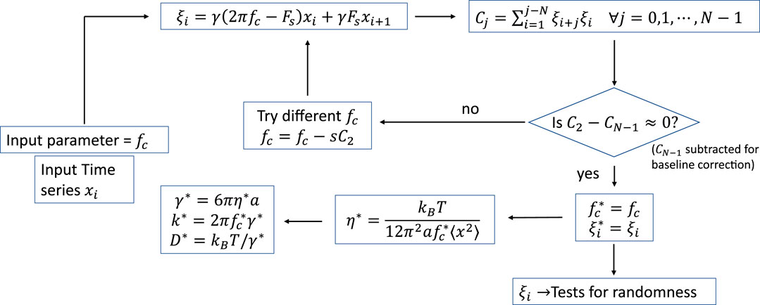
FIGURE 1. Schematic of our algorithm for trap parameter extraction and random number generation.
Our use of the learning algorithm falls in line with the basic philosophy of ML–that is to automate the process and leave less requirement for human intervention. This algorithm can be implemented easily to perform calibration of the optical tweezers in real time [24, 25] which is often necessary in the case of non-equilibrium systems [26, 27]. The main goal is to generate the random numbers; the “training” set is used to optimize the parameters, and then generate the random numbers from the “test” set–which improves upon feeding in more training examples. Additionally, our algorithm can be generalized to a wide range of scenarios, for example calibrating arbitrary potentials, other than the most common harmonic potential studied in this paper. Only the force term in the Langevin Equation will change on generalization, and one has to minimize the deviation of the autocorrelation of the extracted noise from the Dirac delta behavior for all the parameters individually. In addition, this algorithm can be extended to include stochastic motion in viscoelastic fluids, with multiple parameters. Clearly the conventional methods (which are mainly designed for the Markov time-series in harmonic potentials–which is actually a very special case) will be inadequate in these contexts.
We collect position fluctuation data of an optically trapped Brownian particle using a standard optical tweezers setup that is described in detail in Ref. [28]. Here we provide a brief overview for the sake of completeness. Our optical tweezers are built around an inverted microscope (Olympus IX71) with an oil immersion objective lens (Olympus 100 x, 1.3 numerical aperture) and a semiconductor laser (Lasever, 1W max power) of wavelength 1,064 nm which is tightly focused on the sample. We modulate the beam by using the first order diffracted beam off an acousto-optic modulator (AOM, Brimrose) placed at a plane conjugate to the focal plane of the objective lens. The modulation amplitude is small enough such that the power in the first order diffracted beam is modified very minimally (around 1%) as the beam is scanned. We employ a second stationary and co-propagating laser beam of wavelength 780 nm and very low power (
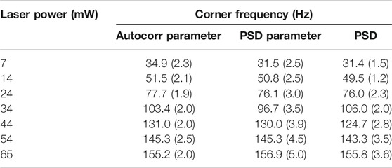
TABLE 1. Variation of corner frequency and related trap stiffness with varying laser power for experiments performed at 5 kHz. The standard deviation for each case is represented in parentheses.
The autocorrelation parameter estimation is directly linked theoretically to the Mean Squared Displacement (MSD) of the data, a measure often exploited to estimate the trap-stiffness. In addition, the Power Spectral Density (PSD) is related to the time-series using a Fourier Transform; further, autocorrelation at short time scales of measurement is related to the PSD by the Weiner-Khinchin theorem as shown in Eq. 4. It can be also related to the Mean Squared displacement (MSD) using time-averaged notation as
Figure 2A shows a typical time series obtained by discrete observations from the position fluctuations of the Brownian particle of diameter
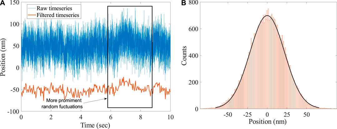
FIGURE 2. (A) Typical time series data of the position fluctuation of an optically trapped Brownian polystyrene bead of radius
This AR (1) variable of probe-displacement is a stationary variable—evident from the measure of the AR coefficient
The squared modulus power of the Fourier Transformed time series follows a Lorentzian function given by Eq. 3. The parameters of this Lorentzian function gives us the required corner frequency. But often, fitting the data becomes a challenge because the fitted parameter values can be sensitive to the region of the fit. So, by following the procedures portrayed in Ref. [19], we bin every 25 points of the Fourier Transformed data. We leave behind the less reliable tail-ends at both high and low frequencies, which are prone to systematic errors. The estimates of the corner frequency using this conventional Power Spectral Density (PSD) are shown in Figures 3A,B for two different laser powers. We made sure that there is no unwanted leakage of the 50 Hz line or its harmonics in the power spectrum, the presence of which can alter the fitted parameters.
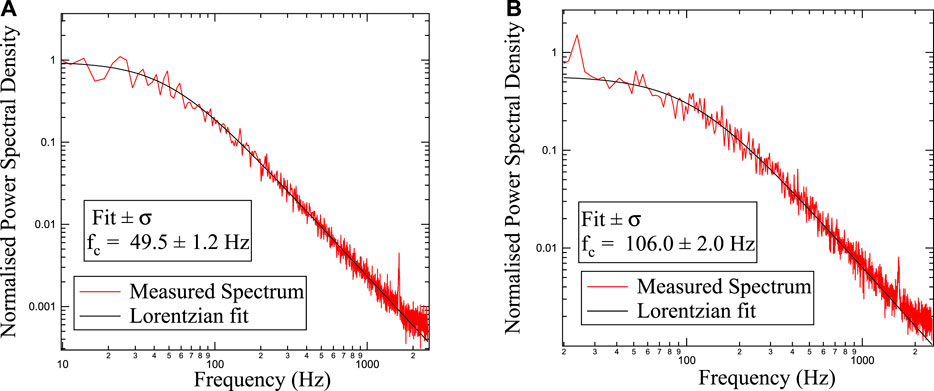
FIGURE 3. Calibration of the trap by fitting a Lorentzian to the power spectral data which has been binned over 25 points. The corner frequencies have been obtained for two different powers, 14 and 34 mW, shown respectively in (A) and (B).
The results obtained in the autocorrelation parameters inference is summarized in Table 1. In Figures 4A,B, the autocorr parameter obtained from the time series after normalization is plotted for two different laser powers. We observe that if the injected
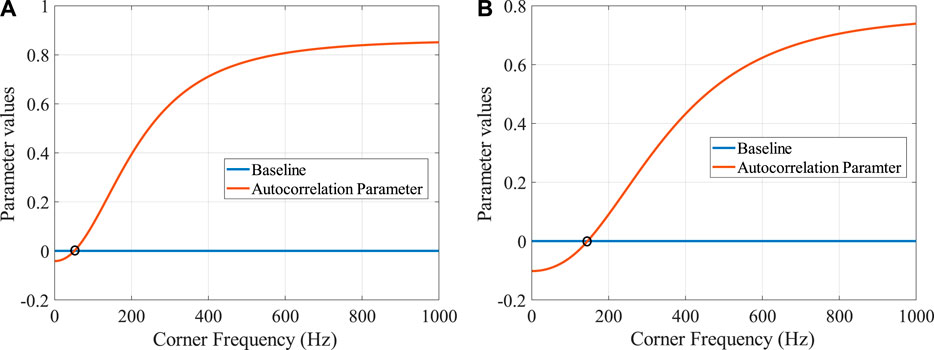
FIGURE 4. Autocorrelation Parameter values plotted for various corner frequencies used as a trail. As stated in the text, we look at the second point from the peak in the Autocorrelation curve. The corner frequency at which this parameter matches the zero baseline can be considered as the correct corner frequency for our system. Figures (A) and (B) are for two different laser powers, 14 and 54 mW, that is two different trap stiffnesses.
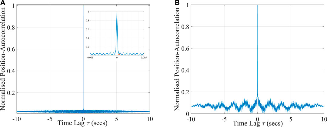
FIGURE 5. Normalized position autocorrelations for various time lags for (A) the extracted random noise, and (B) the Brownian time series. The former shows near perfect temporal delta correlation, the later exhibits exponential decay for small time lags, followed by jittery non-monotonicity.
Every Learning algorithm is based on parameter optimization on a cost function defined by the algorithm. The algorithm minimizes this cost using training examples by optimizing the parameters, which often involves a gradient descent step. Mirroring on the same notion, we define a cost function that essentially is the deviation of the autocorrelation of the extracted noise from the Dirac delta behavior (or the deviation from the flat power spectrum for the noise term). There is no “label” associated with it–indeed, the cost function is calculated from the properties of the input data itself, so it can be classified under an “unsupervized” learning process. We initialize a guess value of the parameter
In Figure 6 we demonstrate a particular scenario for the case where the laser power is 54 mW. Depending on the learning rate, the convergence toward the solution can fast or slow. In Figure 6A two cases are shown where the parameter is initialized at 620 and 30 Hz respectively. The algorithm takes small steps in the direction of the solution until it converges. In Figure 6B
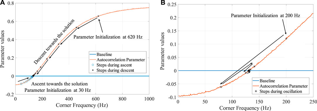
FIGURE 6. The convergence of the parameter value, corner frequency, is shown for two different learning rates, for the case where laser power is 54 mW. After initialization at the trail value the parameter steps toward the zero of the parameter value in small steps. Figure (A) shows the case where learning rate is small, and Figure (B) shows where for a larger learning rate the solution oscillates and moves toward the zero.
We also fit the PSD of each parametrized time series by a straight line in a log scale and note its slope, which we had earlier defined as PSD parameter. The spectrum of a Brownian particle falls as
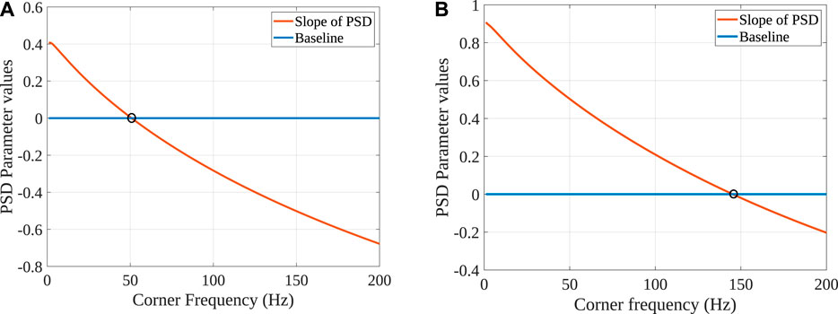
FIGURE 7. Slope of the power spectrum for time series
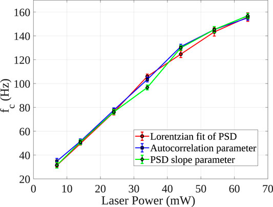
FIGURE 8. Linear variation of corner frequency with laser power, also at lower trapping potentials. The points are plotted with 1σ error bar. Note that the measurements from our method agree very well with that obtained by power spectrum analysis.
In all the columns of Table 1, the figures in parentheses represent the
For the second method (PSD parameter estimation), the errors are again computed from the standard errors associated with fitting the double logarithmic power spectrum vs. frequency curve with a straight line. The errors in fitting are directly related to the error in the estimate of corner frequency. Similarly, the standard error in fitting the binned PSD vs. frequency with the Lorentzian function returns the error in the estimated parameter. Generally, due to the ambient noise sources–systematic errors such as beam pointing fluctuations, laser drifts coupled to our signal are prominent in lower frequencies. So the standard error in the corner frequency measurement is rather large at low corner frequencies.
Viscosity measurement requires spatial calibration of the trap, which we do using “equipartition of energy”. Once the sensitivity measurement is performed, it is easy to estimate η using Eq. 9. Glycerol and water mixed at various concentrations create solutions at different viscosity. Finding η from it requires the variance of the actual time series (which we obtain by fitting the gaussian distribution) and
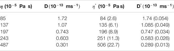
TABLE 2. The first column is the viscosity of the glycerol-water solution (first row only water) as measured in a classical rheometer, while the second column is the diffusion coefficient. The third column provides the viscosity values as obtained in our experiment using Eq. 9, while the fourth column again shows the diffusion coefficient for our case. The standard errors are noted in parentheses.
We now move on to the other aspect of our work: generating unclonable random numbers from the Brownian fluctuations of the optically trapped probe. As stated earlier, the Brownian motion of the particles in water follows Markov dynamics. The motion of the bead in water at any instant is only dependant on the previous instant. In other words, the system stores no memory in the process. The motion of the colloidal particle is a combined manifestation of millions of collisions it has with the ambient water molecules. The Brownian force due to all these collisions is summed up as
The standard deviation of the off-centre values (the autocorrelation values at non-zero time lag) is a good measure of stochasticity. For the best extracted random numbers, we expect to get the least standard deviation. In theory, the deviation should be 0 for perfectly delta correlated numbers, as discussed before. We have sampled our observable at different intervals and compared the standard deviation of the off-centre values. In Figure 9, we observe that with increasing sampling rates, this standard deviation decreases (as expected) until it saturates asymptotically around 2.5 kHz. When the data is sampled over shorter time intervals, fewer effective impacts with the surrounding molecules are averaged; naturally, the stochasticity improves.
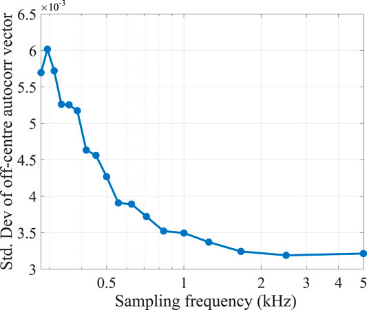
FIGURE 9. The standard deviation of the off-centre values are shown as an inverse measure of randomness; the randomness asymptotically improves with increasing sampling rates.
We proceed to follow the relevant tests of randomness following the NIST-test for randomness suite [22]. We performed all our analyses using
Our null-hypothesis states that the numbers in the time-series are randomly distributed. The alternative hypothesis against this is the opposite, viz. there exists a correlation between successive numbers (and numbers separated by finite a time interval). To test our null hypothesis against the alternative hypothesis, we employ various known statistical methods. Then, we test them against mainly standard-normal, half-normal and chi-squared distributions
In all the NIST sub-tests performed, we have obtained p-values greater than 0.01 which are tabulated in Table 3. This means that the test statistic falls outside the critical region, within the 99% confidence interval of the tests - which implies that we have failed to reject the null hypothesis at a 1% level of significance. Thus, we are more than 99% confident that the array of numbers which we obtain after solving the inverse problem of parameter estimation, is distributed randomly. Additionally, recovering this white-noize term
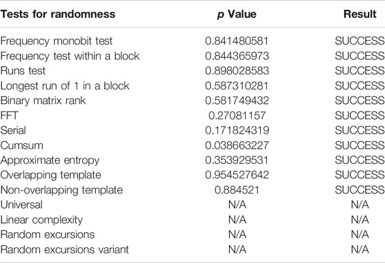
TABLE 3. Results and p values are shown for various tests of randomness provided in the NIST suite. In all the cases, the p-values are greater than 0.01 and result in successful randomness distributions at 99% confidence level. The statistical tests are performed with 40,000 bit long random numbers, N/A corresponds to those tests rendered non applicable due to the requirement of extremely long bit string length
The work we report here serves two primary goals. First and foremost, we describe a new approach to calculate the parameters associated with a confined Brownian motion in a fluid, exploiting the autocorrelation physics of the white noise. A crucial advantage of this method is that it can be implemented “online”, which implies that the parameter can be extracted while recording the data. Any significant fluctuation in the parameter values can be treated as a signature of non-linearity in the system, which precludes the need for further analysis and saves time. Thus, we initially discretize the trajectory of an optically trapped particle into equal-time finite samples, solve the Langevin equation by a finite-difference method, and then construct an inverse problem of parameter extraction by exploiting the temporal delta correlation and flattened nature of the spectral density of the white noise. Thus, we are able to estimate the parameters k (stiffness of the optical trap) and γ (friction constant of the fluid where the particle is immersed) - and use the latter to find out the coefficient of viscosity assuming that the position detection system is pre-calibrated. Our method of parameter estimation is thus virtually immune to electronic noise which is not the case for the other predominantly used methods of calibration such as the Power Spectrum analysis [19] or Equipartition theorem. We observe that the accuracy of the process depends on the number of data points employed, and the entropy of randomness increases with increasing sampling rates. We perform tests for randomness on the extracted time series using the celebrated NIST test suite [22], and observe that our extracted time-series pass all relevant tests at 99% confidence level. Also, since the analysis is solely based on time domain, it has a time complexity of
In summary, our learning algorithm uses “training” a set of incoming data to estimate the trap parameters. These parameters are used in the “test” set to obtain random strings. In future work, we plan to use a similar approach to calibrate the independent parameters of a higher-order AR process, namely Brownian motion in a viscoelastic fluid, which will have non-Markovian features.
The raw data supporting the conclusions of this article will be made available by the authors, without undue reservation.
RD designed the protocol and performed the analysis. SG and AK carried out the experiments. RD and AB both wrote the manuscript as well as planned the project. AB supervised the project.
The authors declare that the research was conducted in the absence of any commercial or financial relationships that could be construed as a potential conflict of interest.
RD would like to thank SERB, Dept of Science and Technology, Govt. of India, for scholarship support under the INSPIRE scheme. SG and AK would like to thank SERB, Dept of Science and Technology, Govt. of India, for fellowship support under the INSPIRE scheme. The authors acknowledge IISER Kolkata, an autonomous teaching and research institution under the Ministry of Human Resource and Development, Govt. of India. RD and AB thank R. K. Nayak and S. Banerjee of the Department of Physical Sciences at IISER-Kolkata for providing valuable insight during several deep discussions.
PSD, power spectral density; Autocorr, autocorrelation; ML, machine learning; MSD, mean squared displacement.
1. Ross SM, Kelly JJ, Sullivan RJ, Perry WJ, Mercer D, Davis RM, et al. Stochastic processes. Vol. 2. New York: Wiley (1996).
3. Steele JM. Stochastic calculus and financial applications. Vol. 45. Springer Science & Business Media (2012).
5. Volpe G, Volpe G. Simulation of a brownian particle in an optical trap. Am J Phys (2013) 81:224–30. doi:10.1119/1.4772632
6. Hu Y, Nualart D. Parameter estimation for fractional ornstein–uhlenbeck processes. Stat Probab Lett (2010) 80:1030–8. doi:10.1016/j.spl.2010.02.018
7. Lewis R, Reinsel GC. Prediction of multivariate time series by autoregressive model fitting. J Multivariate Anal (1985) 16:393–411. doi:10.1111/j.1467-9892.1988.tb00452.x
8. Fällman E, Schedin S, Jass J, Andersson M, Uhlin BE, Axner O. Optical tweezers based force measurement system for quantitating binding interactions: system design and application for the study of bacterial adhesion. Biosens Bioelectron (2004) 19:1429–37. doi:10.1016/j.bios.2003.12.029
9. Keyser U, Van der Does J, Dekker C, Dekker N. Optical tweezers for force measurements on dna in nanopores. Rev Sci Instrum (2006) 77:105105. doi:10.1063/1.2358705
10. Kundu A, Paul S, Banerjee S, Banerjee A. Measurement of van der waals force using oscillating optical tweezers. Appl Phys Lett (2019) 115:123701. doi:10.1063/1.5110581
11. Bera S, Paul S, Singh R, Ghosh D, Kundu A, Banerjee A, et al. Fast bayesian inference of optical trap stiffness and particle diffusion Sci Rep. (2017) 7:1–10. doi:10.1038/srep41638
12. Singh R, Ghosh D, Adhikari R. Fast bayesian inference of the multivariate ornstein-uhlenbeck process. Phys Rev (2018) 98:012136. doi:10.1103/PhysRevE.98.012136
13. Theodoridis S. Probability and stochastic processes. In Machine learning: a bayesian and optimization perspective (2015). 9–51.
14. Aggarwal T, Salapaka M. Real-time nonlinear correction of back-focal-plane detection in optical tweezers. Rev Sci Instrum (2010) 81:123105. doi:10.1063/1.3520463
15. Hart JD, Terashima Y, Uchida A, Baumgartner GB, Murphy TE, Roy R. Recommendations and illustrations for the evaluation of photonic random number generators. APL Photonics (2017) 2:090901. doi:10.1063/1.5000056
16. Keller C, Gürkaynak F, Kaeslin H, Felber N. Dynamic memory-based physically unclonable function for the generation of unique identifiers and true random numbers. In: 2014 IEEE international symposium on circuits and systems (ISCAS); 2014 June 1–5; Melbourne, Australia. IEEE (2014). p. 2740–3.
17. Hu Z, Comeras JM, Park H, Tang J, Afzali A, Tulevski GS, et al. Physically unclonable cryptographic primitives using self-assembled carbon nanotubes Nat Nanotechnol (2016) 11:559. doi:10.1038/nnano.2016.1
19. Berg-Sørensen K, Flyvbjerg H. Power spectrum analysis for optical tweezers. Rev Sci Instrum (2004) 75:594–612. doi:10.1063/1.1645654
20. Neuman KC, Block SM. Optical trapping. Rev Sci Instrum (2004) 75:2787–809. doi:10.1063/1.1785844
21. Doob JL. The brownian movement and stochastic equations. Ann Math (1942) 351–69. doi:10.2307/1968873
22. Rukhin A, Soto J, Nechvatal J, Smid M, Barker E, Leigh S. A statistical test suite for random and pseudorandom number generators for cryptographic applications va Tech. rep. Booz-allen and hamilton inc mclean (2001).
23. Wiener N. Extrapolation, interpolation, and smoothing of stationary time series. The MIT press (1964).
24. Gavrilov M, Jun Y, Bechhoefer J. Real-time calibration of a feedback trap. Rev Sci Instrum (2014) 85:095102. doi:10.1063/1.4894383
25. Jun Y, Gavrilov M, Bechhoefer J. High-precision test of Landauer's principle in a feedback trap. Phys Rev Lett (2014) 113:190601. doi:10.1103/PhysRevLett.113.190601
26. Martínez IA, Roldán É, Dinis L, Petrov D, Parrondo JMR, Rica RA. Brownian carnot engine. Nat Phys (2016) 12:67–70. doi:10.1038/NPHYS3518
27. Blickle V, Bechinger C. Realization of a micrometre-sized stochastic heat engine. Nat Phys (2012) 8:143–6. doi:10.1038/nphys2163
28. Pal SB, Haldar A, Roy B, Banerjee A. Measurement of probe displacement to the thermal resolution limit in photonic force microscopy using a miniature quadrant photodetector. Rev Sci Instrum (2012) 83:023108. doi:10.1063/1.3685616
29. Shumway RH, Stoffer DS. Time series analysis and its applications: with R examples. Springer (2017).
30. Li T, Raizen MG. Brownian motion at short time scales. Ann Phys (2013) 525:281–95. doi:10.1002/andp.201200232
31. Grimm M, Franosch T, Jeney S. High-resolution detection of brownian motion for quantitative optical tweezers experiments. Phys Rev E Stat Nonlinear Soft Matter Phys (2012) 86:021912. doi:10.1103/PhysRevE.86.021912
32. Stasev YV, Kuznetsov A, Nosik A. Formation of pseudorandom sequences with improved autocorrelation properties. Cybern Syst Anal (2007) 43:1–11. doi:10.1007/s10559-007-0021-2
33. Simpson H. Statistical properties of a class of pseudorandom sequences. Proc Inst Electr Eng (1966) 113:2075–80. doi:10.1049/piee.1966.0361
Keywords: true random numbers, supervised learning, optical trap calibration, autoregresison, time series analysis
Citation: Dey R, Ghosh S, Kundu A and Banerjee A (2021) Simultaneous Random Number Generation and Optical Tweezers Calibration Employing a Learning Algorithm Based on the Brownian Dynamics of a Trapped Colloidal Particle. Front. Phys. 8:576948. doi: 10.3389/fphy.2020.576948
Received: 27 June 2020; Accepted: 01 December 2020;
Published: 15 January 2021.
Edited by:
Daryl Preece, University of California, San Diego, United StatesReviewed by:
Ilia L. Rasskazov, University of Rochester, United StatesCopyright © 2021 Dey, Ghosh, Kundu and Banerjee. This is an open-access article distributed under the terms of the Creative Commons Attribution License (CC BY). The use, distribution or reproduction in other forums is permitted, provided the original author(s) and the copyright owner(s) are credited and that the original publication in this journal is cited, in accordance with accepted academic practice. No use, distribution or reproduction is permitted which does not comply with these terms.
*Correspondence: Ayan Banerjee, YXlhbkBpaXNlcmtvbC5hYy5pbg==
Disclaimer: All claims expressed in this article are solely those of the authors and do not necessarily represent those of their affiliated organizations, or those of the publisher, the editors and the reviewers. Any product that may be evaluated in this article or claim that may be made by its manufacturer is not guaranteed or endorsed by the publisher.
Research integrity at Frontiers
Learn more about the work of our research integrity team to safeguard the quality of each article we publish.