An Efficient Numerical Technique for Solving Time-Fractional Generalized Fisher's Equation

This paper extends the existing Fisher's equation by adding the source term and generalizing the degree β of the non-linear part. A numerical solution of a modified Fisher's equation for different values of β using the cubic B-spline collocation scheme is also investigated. The fractional derivative in a time dimension is discretized in Caputo's form based on the L1 formula, while cubic B-spline basis functions are used to interpolate the spatial derivative. The non-linear part in the model is linearized by the modified formula. The efficiency of the proposed scheme is examined by simulating four test examples with different initial and boundary conditions. The effect of different parameters is discussed and presented in tables and graphics form. Moreover, by using the Von Neumann stability formula, the proposed scheme is shown to be unconditionally stable. The results of error norms reflect that the present scheme is suitable for non-linear time fractional differential equations.

1. Introduction

Fractional calculus-based models have been used in different fields of engineering and science. In the last few years, fractional differential equations have been widely used. The main advantage of using fractional order differential equation is its non-local property in mathematical modeling. During the twentieth century, the authors [1–3] added a significant amount of research in the area of fractional calculus. The applications can be seen in different branches of science and engineering, such as finance [4], nano-technology [5], electrodynamics [6], and visco-elasticity. Fisher's equation is commonly used in epidemics and bacteria, branching Brownian motion, neolithic transitions and chemical kinetics [7–9]. The spatial and temporal propagation of a virile gene in an infinite medium has been explained by Fisher [10]. Several numerical methods for differential equations with Riemann-Liouville and Caputo sense fractional order derivatives have been applied and analyzed [11–13].

The time-fractional Fisher's equation used in Baranwal et al. [14] has been modified in this paper in two different ways: (1) by introducing the source term or (2) by generalizing the non-linear power.

The modified form of time fractional Fisher's equation is:

$\begin{array}{l}\frac{{\partial }^{\alpha }Z(r,t)}{\partial t^{\alpha }}-\nu \frac{{\partial }^{2}Z(r,t)}{\partial r^2}-Z(r,t)(1-Z^{\beta }(r,t))\\ =f(r,t),a\le r\le b,0<\alpha \le 1,t\ge 0,& (1.1)\end{array}$

with the initial condition

$\begin{array}{ll}Z(r,0)=\psi (r),a\le r\le b,& (1.2)\end{array}$

and the boundary conditions

$\begin{array}{ll}Z(a,t)={\psi }_1(t),Z(b,t)={\psi }_2(t),t\ge 0,& (1.3)\end{array}$

where ν is a parameter of viscosity.

The Caputo and Riemann-Liouville fractional derivatives have a wide range of applications [15–17]. The Caputo derivative is used in this work:

$\begin{array}{l}\frac{{\partial }^{\alpha }Z(r,t)}{\partial t^{\alpha }}=\{\begin{array}{cc}\frac{1}{\Gamma (q-a)}{\int }_0^t\frac{{\partial }^{q}Z(r,s)}{\partial t^q}{(t-s)}^{q-\alpha -1}ds,\hfill & q-1<\alpha <q,\\ \frac{{\partial }^{q}Z(r,t)}{\partial t^q},\hfill & q=\alpha .\end{array}\end{array}$

The Caputo derivative is discretized by the L1 formula [18]:

$\begin{array}{ll}\frac{{\partial }^{\alpha }h}{\partial t^{\alpha }}|t_n=\frac{1}{{(\Delta t)}^{\alpha }\Gamma (2-\alpha )}{\displaystyle \sum _{k=0}^{n-1}}{\lambda }_k^{\alpha }\left[h(t_{n-k})-h(t_{n-k-1})\right]+O(\Delta t),& (1.4)\end{array}$

where ${\lambda }_k={(k+1)}^{1-\alpha }-k^{1-\alpha }$.

In this paper, we generalized the linearization formula used in [19]:

$\begin{array}{ll}{(Z^{\beta })}_j^{n+1}=\beta Z_j^{n+1}{(Z^{\beta -1})}_j^n-(\beta -1){(Z^{\beta })}_j^n,& (1.5)\end{array}$

where β is a positive integer.

The numerical and analytical solution of fractional order PDEs play an important role in explaining the characteristics of non-linear problems that arise in everyday life. In the literature, researchers applied various techniques for the numerical solutions of Fisher's equation. Baranwal et al. [14] introduced an analytic algorithm for solving non-linear time-fractional reaction diffusion equations based on the variational iteration method (VIM) and Adomian decomposition method (ADM). Wazwaz and Gorguis [20] implemented ADM for the analytic study of Fisher's equation. Homotopy perturbation sumudu transform method has been applied for solving fractional non-linear dispersive equations by Abedle-Rady et al. [21]. Gupta and Saha Ray [22] implemented two methods. Haar wavelet method and the optimal homotopy asymptotic method (OHAM) for the numerical solutions of arbitrary order PDE, such as Burger-Fisher's and generalized Fisher's equations. Cherif et al. [23] solved space-fractional Fisher's equation using classical HPM. Khader and Saad [24] proposed a numerical solution for solving the space-fractional Fisher's equation using Chebyshev spectral collocation technique. Rawashdeh [25] introduced the fractional natural decomposition method (FNDM) to find the analytical and approximate solutions of the non-linear time-fractional Harry Dym equation and the non-linear time-fractional Fisher's equation. Singh [26] introduced an efficient computational method for the approximate solution of a non-linear Lane-Emden-type equation. The numerical solution of fractional vibration equation of large membrane has been investigated in Singh [27] by Jacobi polynomial. The authors in [28] employed the cubic B-spline method for the numerical simulations of time fractional Burgers' and Fisher's equation. Singh et al. [29] constructed a q-homotopy analysis transform method for solving time and space-fractional coupled Burgers' equation. Najeeb et al. [30] used HPM for the analytical solution of time-fractional reaction-diffusion equation. Majeed et al. [28] used B-spline at non-uniform for the construction of craniofacial fractures.

In this paper, we have presented a cubic B-spline (CBS) algorithm for numerical simulation of the time-fractional generalized Fisher's equation. Caputo's time fractional derivative based on the L1 scheme has been discretized by finite difference formula, whereas spatial derivatives are discretized by CBS functions. The present approach is novel for the numerical results of fractional order PDEs and, to the best of our knowledge, any spline solution of the time-fractional generalized Fisher's equation has never yet been studied. Moreover, this scheme is equally effective for homogeneous and non-homogeneous boundary conditions.

This article has been presented in the following manner. Section 2 evolves a brief description of temporal discretization, cubic B-spline functions and spatial discretization. In section 4, the stability of the proposed algorithm has been discussed. The discussion on numerical results of four test problems has been reported in section 5. Concluding remarks of this work are given in section 6.

2. Description of the Method

Let us consider the interval [a, b] is sub divided into N finite elements of equal spacing h determined by the knots r_j, j = 0, 1, 2, 3.……, N such that a = r₀ < r₁ < r₂… < r_N−1 < r_N = b. The cubic B-spline basis function at the grid points is defined as

$\begin{array}{ll}{\varphi }_j(r)=\frac{1}{6h^3}\{\begin{array}{l}{(r-r_j)}^3,\text{if }r\in [r_j,r_{j+1}),\\ h^3+3h^2(r-r_{j+1})\\ +3h{(r-r_{j+1})}^2-3{(r-r_{j+1})}^3,\text{if }r\in [r_{j+1},r_{j+2}],\\ h^3+3h^2(r_{j+3}-r)\\ +3h{(r_{j+3}-r)}^2-3{(r_{j+3}-r)}^3,\text{if }r\in [r_{j+2},r_{j+3}],\\ {(r_{j+4}-r)}^3,\text{if }r\in [r_{j+3},r_{j+4}).\end{array}& (2.1)\end{array}$

From the above basis, the approximation solution Z_N(r, t) can be written in terms of linear combination of cubic B-spline base function as follows

$\begin{array}{ll}{Z}_N(r,t)={\displaystyle \sum _{j=-1}^{N+1}}{{\rm Y}}_j(t){\varphi }_j(r),& (2.2)\end{array}$

where ${{\rm Y}}_j{(t)}^{\prime }s$ are the unknowns to be determined. Four consecutive cubic B-splines are used to construct each element [r_j, r_j+1]. The values of cubic B-splines and its derivatives at the nodal points are given in Table 1. The variation of Z_N(r, t) over the typical component [r_j, r_j+1] is given by

$\begin{array}{ll}{Z}_N(r_j,t_n)={\displaystyle \sum _{m=j-1}^{j+1}}{{\rm Y}}_m(t){\varphi }_m(r_m).& (2.3)\end{array}$

TABLE 1

Table 1. Coefficients of CBS and its derivative at the nodes r_j.

By plugging the approximation values given in Table 1 into Equation (2.3) at (r_j, t_n), The Equation (1.1) yields the following set of fractional order ordinary differential equations.

$\begin{array}{l}\left[({{\rm Y}}_{j-1}^{•}(t)+4{{\rm Y}}_j^{•}(t)+{{\rm Y}}_{j+1}^{•}(t))/6\right]-\frac{\nu }{h^2}\left[{{\rm Y}}_{j-1}-2{{\rm Y}}_j+{{\rm Y}}_{j+1}\right]\\ -\left[({{\rm Y}}_{j-1}+4{{\rm Y}}_j+{{\rm Y}}_{j+1})/6\right]\left[1-{(({{\rm Y}}_{j-1}+4{{\rm Y}}_j+{{\rm Y}}_{j+1})/6)}^{\beta }\right]\\ =f(r_j,t_n).& (2.4)\end{array}$

Here, • represents αth order fractional derivative with respect to time. After some simplification, a recurrence relation for Equation (1.1) with β = 3 can be written as

$\begin{array}{l}{{\rm Y}}_{j-1}^{n+1}\left[\frac{\gamma }{6}-\frac{1}{2h^2}-\frac{1}{12}+\frac{2}{1296}{(T_m)}^3\right]\\ +{{\rm Y}}_j^{n+1}\left[\frac{4\gamma }{6}+\frac{1}{h^2}-\frac{1}{3}+\frac{8}{1296}{(T_m)}^3\right]\\ +{{\rm Y}}_{j+1}^{n+1}\left[\frac{\gamma }{6}-\frac{1}{2h^2}-\frac{1}{12}+\frac{2}{1296}{(T_m)}^3\right]\\ ={{\rm Y}}_{j-1}^n\left[\frac{\gamma }{6}+\frac{1}{2h^2}+\frac{1}{12}\right]+{{\rm Y}}_j^n\left[\frac{4\gamma }{6}-\frac{1}{h^2}+\frac{1}{3}\right]\\ +{{\rm Y}}_{j+1}^n\left[\frac{\gamma }{6}+\frac{1}{2h^2}+\frac{1}{12}\right]-\frac{1}{1296}{(T_m)}^4+f(r_j,t_n)\\ -(\gamma {\displaystyle \sum _{k=0}^{n-1}{\lambda }_k}[(({{\rm Y}}_{j-1}^{n-k-1}-{{\rm Y}}_{j-1}^{n-k})+4({{\rm Y}}_j^{n-k-1}-{{\rm Y}}_j^{n-k})\\ +({{\rm Y}}_{j+1}^{n-k-1}-{{\rm Y}}_{j+1}^{n-k}))/6]+{\rho }_{\Delta t}^{n+1}),& (2.5)\end{array}$

where ${\lambda }_k=\left[{(k+1)}^{1-\alpha }-k^{1-\alpha }\right],$ $T_m={{\rm Y}}_{j-1}^n+4{{\rm Y}}_j^n+{{\rm Y}}_{j+1}^n,$ $\gamma =\frac{{(\Delta t)}^{-\alpha }}{\Gamma (2-\alpha )}$. Moreover, the truncation error ${\rho }_{\Delta t}^{n+1}$ is bounded as

$\begin{array}{ll}\left|{\rho }_{\Delta t}^{n+1}\right|\le \varpi {(\Delta t)}^{2-\alpha },& (2.6)\end{array}$

where ϖ is a real constant.

Lemma 2.1. The coefficients λ_k in (2.5) possess the following characteristics [31]:

• λ_k > 0 and λ₀ = 1, k = 1:1:n,

• λ₀ > λ₁ > λ₂ > … > λ_k, λ_k → 0 as k → ∞,

• $\sum _{k=0}^n({\lambda }_k-{\lambda }_{k+1})+{\lambda }_{n+1}=(1-{\lambda }_1)+\sum _{k=1}^{n-1}({\lambda }_k-{\lambda }_{k+1})+{\lambda }_n=1$.

Equation (2.5) is modified as

$\begin{array}{l}{{\rm Y}}_{j-1}^{n+1}{\alpha }_0+{{\rm Y}}_j^{n+1}{\alpha }_1+{{\rm Y}}_{j+1}^{n+1}{\alpha }_0={{\rm Y}}_{j-1}^n(n_1)+{{\rm Y}}_j^n(n_2)\\ +{{\rm Y}}_{j+1}^n(n_1)-\frac{1}{1296}{(T_m)}^4+f(r_j,t_n)\\ -(\gamma {\displaystyle \sum _{k=1}^{n-1}{\lambda }_k}[(({{\rm Y}}_{j-1}^{n-k-1}-{{\rm Y}}_{j-1}^{n-k})+4({{\rm Y}}_j^{n-k-1}-{{\rm Y}}_j^{n-k})\\ +({{\rm Y}}_{j+1}^{n-k-1}-{{\rm Y}}_{j+1}^{n-k}))/6]+{\rho }_{\Delta t}^{n+1}),& (2.7)\end{array}$

where ${\alpha }_0=\frac{\gamma }{6}-\frac{1}{2h^2}-\frac{1}{12}+\frac{2}{1296}{(T_m)}^3,{\alpha }_1=\frac{4\gamma }{6}+\frac{1}{h^2}-\frac{1}{3}+\frac{8}{1296}{(T_m)}^3,$ $n_1=\frac{\gamma }{6}+\frac{1}{2h^2}+\frac{1}{12}$ and $n_2=\frac{4\gamma }{6}-\frac{1}{h^2}+\frac{1}{3}$

From (2.7), the system of N + 1 linear equation with N + 3 unknown parameters ${({{\rm Y}}_{-1},{{\rm Y}}_0,{{\rm Y}}_1,\dots ,{{\rm Y}}_{N+1})}^T$ can be obtained. To acquire unique solution of the system, two extra equations are needed. For this purpose, given boundary conditions are used. Thus, the system of linear equations for expression (2.7) becomes

$\begin{array}{ll}P{Y}^{n+1}=Q{Y}^n.& (2.8)\end{array}$

$\begin{array}{l}{Y}^n={({{\rm Y}}_{-1}^n,{{\rm Y}}_0^n,{{\rm Y}}_1^n,\dots ,{{\rm Y}}_{N+1}^n)}^T.\end{array}$

where

$\begin{array}{ll}P=\left[\begin{array}{cccccccc}\frac{1}{6}& \frac{4}{6}& \frac{1}{6}& 0& \cdots & 0& 0& 0\\ {\alpha }_0& {\alpha }_1& {\alpha }_0& 0& \cdots & 0& 0& 0\\ ⋮& ⋮& ⋮& ⋮& \ddots & ⋮& ⋮& ⋮\\ 0& 0& 0& 0& \cdots & {\alpha }_0& {\alpha }_1& {\alpha }_0\\ 0& 0& 0& 0& \cdots & \frac{1}{6}& \frac{4}{6}& \frac{1}{6}\end{array}\right].& (2.9)\end{array}$

3. Initial Vector

For the initial vector, the initial and boundary conditions of the problem under consideration will help to compute the initial vector $Y^0={({{\rm Y}}_{-1}^0,{{\rm Y}}_0^0,{{\rm Y}}_1^0,\dots ,{{\rm Y}}_{N+1}^0)}^T$. The approximation (2.2) therefore becomes

$\begin{array}{l}{Z}_N(r,0)={\displaystyle \sum _{j=-1}^{N+1}}{{\rm Y}}_j(0){\varphi }_j(r).\end{array}$

To determine Υ⁰, the approximation for the derivatives of the initial and boundary conditions is as follows [32]:

• ${(Z_r)}_j^k=g^{\prime }(r_j)$ for j = 0, N

• ${(Z)}_j^0=g(r_j)$ for j = 0, 1, 2, …, N

This gives the following (N + 3) × (N + 3) matrix system:

$\begin{array}{l}\left[\begin{array}{cccccccc}\frac{-1}{2h}& 0& \frac{1}{2h}& 0& \cdots & 0& 0& 0\\ \frac{1}{6}& \frac{4}{6}& \frac{1}{6}& 0& \cdots & 0& 0& 0\\ ⋮& ⋮& ⋮& ⋮& \ddots & ⋮& ⋮& ⋮\\ 0& 0& 0& 0& \cdots & \frac{1}{6}& \frac{4}{6}& \frac{1}{6}\\ 0& 0& 0& 0& \cdots & \frac{-1}{2h}& 0& \frac{1}{2h}\end{array}\right]\left[\begin{array}{c}{{\rm Y}}_{-1}^0\\ {{\rm Y}}_0^0\\ ⋮\\ {{\rm Y}}_{N+1}^0\end{array}\right]=\left[\begin{array}{c}{g}^{\prime }(r_0)\\ g(r_0)\\ ⋮\\ g(r_N)\\ g^{\prime }(r_N)\end{array}\right]\end{array}$

4. Stability Analysis

The von Neumann analysis is frequently used to determine the requirements of stability, as it is usually simple to apply in a simple way. The solution in single Fourier mode is defined as

$\begin{array}{ll}{{\rm Y}}_j^n={{\rm Y}}^k{e}^{i\eta jh},& (4.1)\end{array}$

where $i=\sqrt{-1}$. The approximation solution of generalized Fisher's equation (2.7) can be written as

$\begin{array}{l}{{\rm Y}}_{j-1}^{n+1}({\alpha }_0)+{{\rm Y}}_j^{n+1}({\alpha }_1)+{{\rm Y}}_{j+1}^{n+1}({\alpha }_0)={{\rm Y}}_{j-1}^n(n_1)+{{\rm Y}}_j^n(n_2)\\ +{{\rm Y}}_{j+1}^n(n_3)-\frac{1}{1296}{(T_m)}^4\\ +f(r_j,t_n)-\gamma {\displaystyle \sum _{k=1}^{n-1}{\lambda }_k^{\alpha }}[(({{\rm Y}}_{j-1}^{n-k+1}-{{\rm Y}}_{j-1}^{n-k})\\ +4({{\rm Y}}_j^{n-k+1}-{{\rm Y}}_j^{n-k})+({{\rm Y}}_{j+1}^{n-k+1}-{{\rm Y}}_{j+1}^{n-k}))/6].& (4.2)\end{array}$

where $n_1=\frac{\gamma }{6}+\frac{1}{2h^2}+\frac{1}{12},n_2=\frac{4\gamma }{6}-\frac{1}{h^2}+\frac{1}{3},n_3=\frac{\gamma }{6}$ $+\frac{1}{2h^2}+\frac{1}{12},$ $T_m={{\rm Y}}_{i-1}^n+4{{\rm Y}}_i^n+{{\rm Y}}_{i+1}^n.$

Substituting (4.1) into (4.2), we get

$\begin{array}{l}{{\rm Y}}^{k+1}{e}^{i\eta (j-1)h}({\alpha }_0)+{{\rm Y}}^{k+1}{e}^{i\eta (j)h}({\alpha }_1)+{{\rm Y}}^{k+1}{e}^{i\eta (j+1)h}({\alpha }_0)\\ ={{\rm Y}}^k{e}^{i\eta (j-1)h}(n_1)\\ +{{\rm Y}}^k{e}^{i\eta (j)h}(n_2)+{{\rm Y}}^k{e}^{i\eta (j+1)h}(n_3)-\frac{1}{1296}{(T_m)}^4+f(r,t)\\ -{\displaystyle \sum _{k=1}^{n-1}{\lambda }_k^{\alpha }}[(({{\rm Y}}^{n-k+1}{e}^{i\eta (j-1)h}\\ -{{\rm Y}}^{n-k}{e}^{i\eta (j-1)h})+4({{\rm Y}}^{n-k+1}{e}^{i\eta (j)h}-{{\rm Y}}^{n-k}{e}^{i\eta (j)h})\\ +({{\rm Y}}^{n-k+1}{e}^{i\eta (j+1)h}-{{\rm Y}}^{n-k}{e}^{i\eta (j+1)h}))/6].\end{array}$

$\begin{array}{l}{{\rm Y}}^{k+1}[e^{i\eta (j-1)h}({\alpha }_0)+e^{i\eta (j)h}({\alpha }_1)+e^{i\eta (j+1)h}({\alpha }_0)]\\ ={{\rm Y}}^k[e^{i\eta (j-1)h}(n_1)+e^{i\eta (j)h}(n_2)\\ +e^{i\eta (j+1)h}(n_3)]-\frac{1}{1296}{(T_m)}^4+f(r,t)\\ -{\displaystyle \sum _{k=1}^{n-1}{\lambda }_k^{\alpha }}[({{\rm Y}}^{n-k+1}{e}^{i\eta (j-1)h}-{{\rm Y}}^{n-k}{e}^{i\eta (j-1)h}\\ +4{{\rm Y}}^{n-k+1}{e}^{i\eta (j)h}-4{{\rm Y}}^{n-k}{e}^{i\eta (j)h}+{{\rm Y}}^{n-k+1}{e}^{i\eta (j+1)h}\\ -{{\rm Y}}^{n-k}{e}^{i\eta (j+1)h})/6].\end{array}$

$\begin{array}{l}{{\rm Y}}^{k+1}=\frac{{{\rm Y}}^k{e}^{i\eta (j)h}[e^{-i\eta h}(n_1)+n_2+e^{i\eta h}(n_3)]-\frac{1}{1296}{(T_m)}^4{e}^{-i\eta jh}+f(r,t)e^{-i\eta jh}}{e^{i\eta (j)h}[e^{-i\eta h}({\alpha }_0)+{\alpha }_1+e^{i\eta h}({\alpha }_0)]}\\ -\frac{{\displaystyle {\sum }_{k=1}^{n-1}{\lambda }_k^{\alpha }}[{{\rm Y}}^{n-k+1}{e}^{i\eta jh}(e^{-i\eta h}+4+e^{i\eta h})-{{\rm Y}}^{n-k}{e}^{-i\eta jh}(e^{-i\eta h}+4+e^{i\eta h})]}{e^{i\eta (j)h}[e^{-i\eta h}({\alpha }_0)+{\alpha }_1+e^{i\eta h}({\alpha }_0)]}.\end{array}$

By inserting values of α₀, α₁ and n₁, n₂, n₃ in above expression, we have

$\begin{array}{l}{{\rm Y}}^{k+1}=\frac{{{\rm Y}}^k\left[\frac{\gamma }{3}(cos\eta h+3)+\frac{1}{6h^2}(cos\eta h-6)+\frac{1}{6}(cos\eta h+2)\right]-\frac{1}{1296}{(T_m)}^4{e}^{-i\eta jh}}{\frac{\gamma }{3}(cos\eta h+3)-\frac{1}{6h^2}(cos\eta h-6)-\frac{1}{6}(cos\eta h+2)+\frac{3}{216}{(T_m)}^2(cos\eta h+3)}\\ +\frac{f(r,t)e^{-i\eta jh}-{\displaystyle {\sum }_{k=1}^{n-1}}{\lambda }_k^{\alpha }\left[2cos\eta h+4({{\rm Y}}^{n-k+1}-{{\rm Y}}^{n-k})\right]}{\frac{\gamma }{3}(cos\eta h+3)-\frac{1}{6h^2}(cos\eta h-6)-\frac{1}{6}(cos\eta h+2)+\frac{3}{216}{(T_m)}^2(cos\eta h+3)}.\end{array}$

The applied scheme is stable if augment factor |Υ^k+1| ≤ 1, and, from the above expression, we can observe that value of numerator is lesser than denominator for the values of γ, η, h. The scheme become unstable as the approximations grows in magnitude.

${{\rm Y}}^{k+1}\le {{\rm Y}}^k,$

${{\rm Y}}^{k+1}\le 1.$

The above result thus reflects that scheme is unconditionally stable.

5. Applications and Discussion

This section presents some examples with different initial and boundary conditions. The numerical results are presented graphically and numerically in figures and tables. The error norms L² and L^∞ are computed to analyze the precision of the suggested technique as

$\begin{array}{l}{L}^2=\parallel Z_{exact}-Z_{approx}{\parallel }_2\simeq \sqrt{h{\displaystyle \sum _{j=0}^n}|{(Z_j)}_{exact}-{(Z_j)}_{approx}{|}^2},\end{array}$

$\begin{array}{l}{L}^{\infty }=\parallel Z_{exact}-Z_{approx}{\parallel }_{\infty }\simeq ma{x}_j\mid {(Z_j)}_{exact}-{(Z_j)}_{approx}\mid .\end{array}$

In this manuscript we used, MATLAB 2015b on Intel^RCORE^TMi5 CPU with 8GB RAM and 64-bit operating system (window 7) for numerical simulations.

Example 5.1. Consider the fractional order Fisher's equation (1.1) for β = 3 subject to

$\begin{array}{ll}\frac{{\partial }^{\alpha }Z(r,t)}{\partial t^{\alpha }}-\nu \frac{{\partial }^{2}Z(r,t)}{\partial r^2}-Z(r,t)(1-Z^3(r,t))=f(r,t).& (5.1)\end{array}$

$\begin{array}{l}IC:Z(r,0)=0,0\le r\le 1.\end{array}$

$\begin{array}{l}BCs:Z(0,t)=t^{2\alpha },Z(1,t)=0,t\ge 0.\end{array}$

and the source term

$\begin{array}{l}\begin{array}{r}f(r,t)=exp(2r)(1-r^2)t^{\alpha }\frac{\Gamma (2\alpha +1)}{\Gamma (1+\alpha )}-2\nu t^{2\alpha }(1-4r-2r^2)exp(2r)\\ -[t^{2\alpha }(1-r^2)exp(2r)][1-{(t^{2\alpha }(1-r^2)exp(2r))}^3].\end{array}\end{array}$

The approximate solution (2.3) can be written in piecewise form:

$\begin{array}{l}Z(r,t_n)={{\rm Y}}_{j-3}{\varphi }_{3,j-3}(r)+{{\rm Y}}_{j-2}{\varphi }_{3,j-2}(r)\\ +{{\rm Y}}_{j-1}{\varphi }_{3,j-1}(r)+{{\rm Y}}_j{\varphi }_{3,j}(r),r\in [r_j,r_{j+1}).& (5.2)\end{array}$

$\begin{array}{ll}{Z}_N(r,1)=\{\begin{array}{c}{r}^3-0.64r^2-0.805r+0.99997,r\in [0,0.1),\\ 0.56667r^3-0.51r^2-0.818r+1.0004,r\in [0.1,0.2),\\ 16.75r^3-10.22r^2+1.124r+0.87093,r\in [0.2,0.3),\\ 0.11667r^3-0.195r^2-0.8945r+1.0068,r\in [0.3,0.4),\\ -0.033333r^3-0.015r^2-0.9665r+1.0165,r\in [0.4,0.5),\\ -0.066667r^3+0.035r^2-0.9915r+1.0206,r\in [0.5,0.6),\\ -0.05r^3+0.005r^2-0.9735r+1.017,r\in [0.6,0.7),\\ -0.033333r^3-0.03r^2-0.949r+1.0113,r\in [0.7,0.8),\\ -3546.6r^3+8511.7r^2-6810.3r+1816.8,r\in [0.8,0.9),\\ 10640.0r^3-29793.0r^2+27664.0r-8525.4,r\in [0.9,1).\end{array}\hfill & (5.3)\end{array}$

The exact solution of (5.1) is Z(r, t) = t^2α(1 − r²)exp(2r).

Figures 1, 2 explores the comparison of CBS solution with exact solution for Example 5.1 for different parameters. Figure 1A shows the 2-dimensional preview of approximate and exact results for t = 0.25 with α = 0.95, h = 0.01, Δt = 0.0003 and ν = 1. The graph illustrates that exact and approximate outcomes are indiscriminately similar to each other. Figure 1B cites the action of solution obtained for Equation (5.1) with α = 0.95, h = 0.01, ν = 1 and for various time steps t = 0.5, 0.75, and 1 with Δt = 0.0003. It is clear from the graph that both solutions are overlapping. Three dimensional preview has been given in Figure 2. While the influence of α has been discussed for distinct Brownian motion, i.e, α = 0.25, 0.5, and 0.98 in Figure 3. It can be observed that as the value of α increases, the solution profile decreases and as α → 1, the numerical solution tends to overlap the exact solution. The comparison of numerical and exact outcomes is expressed in Table 2, which shows that both results are consistent with each other and are accurate up to 5 decimal places. The numerical results for α variation is presented in Table 3. It is clear from tabular data that both results strongly agree with each other, and the accuracy of the scheme is examined by the error norms as shown in Table 4.

FIGURE 1

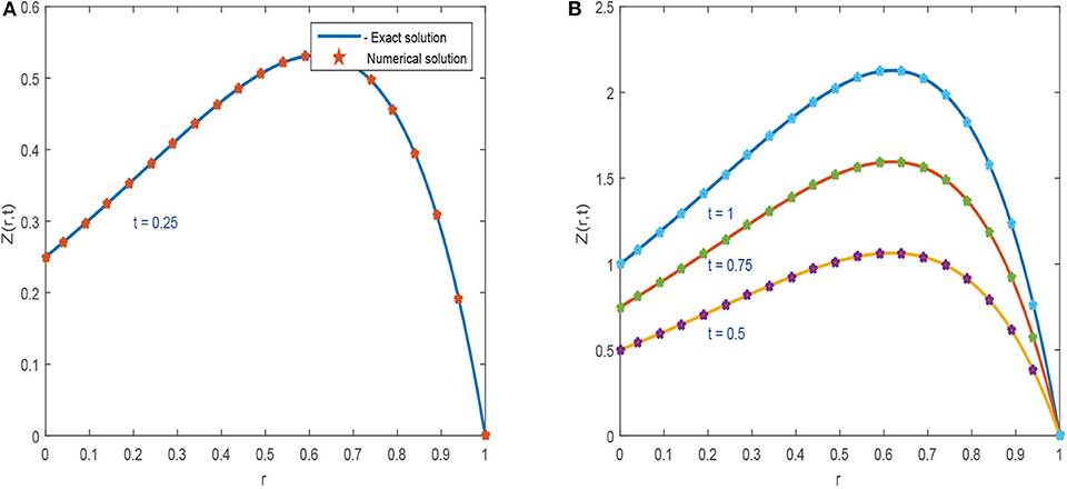
Figure 1. Approximate results of Example 5.1 at different time levels for α = 0.95, ν = 1, Δt = 0.0003, and h = 0.01. (A) For t = 0.25. (B) For t = 0.5, 0.75, and 1.

FIGURE 2

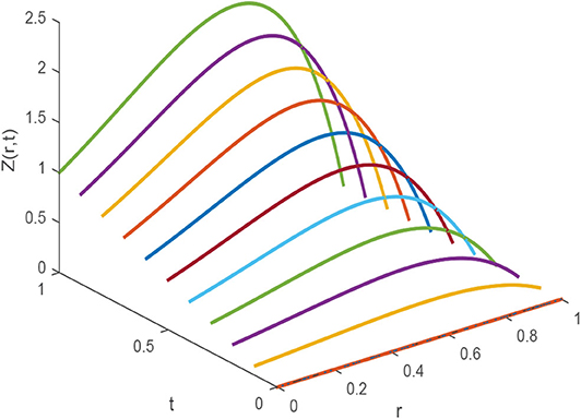
Figure 2. 3D image of numerical solution of Example 5.1 for t ϵ [0, 1], α = 0.25, ν = 1, Δt = 0.0003, and h = 0.01.

FIGURE 3

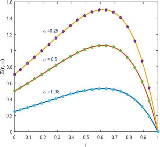
Figure 3. Numerical solution of Example 5.1 for various values of α = 0.25, 0.5, and 0.98, ν = 1, Δt = 0.0003, and h = 0.01.

TABLE 2

Table 2. The comparison of results for Example 5.1 at different time level.

TABLE 3

Table 3. The comparison of results for Example 5.1 at different values of α and t = 0.5.

TABLE 4

Table 4. Computation of error norms for Example 5.1.

Example 5.2. The fractional order Fisher's equation (1.1) for β = 3 can be written as:

$\begin{array}{ll}\frac{{\partial }^{\alpha }Z(r,t)}{\partial t^{\alpha }}-\nu \frac{{\partial }^{2}Z(r,t)}{\partial r^2}-Z(r,t)(1-Z^3(r,t))=f(r,t).& (5.4)\end{array}$

with

$\begin{array}{l}IC:Z(r,0)=r^{2}exp(2r),0\le r\le 1.\end{array}$

$\begin{array}{l}BCs:Z(0,t)=0,Z(1,t)=exp(2)(1+t^2),t\ge 0.\end{array}$

source term is

$\begin{array}{l}\begin{array}{r}f(r,t)=\frac{2r^2{t}^{2-\alpha }exp(2r)}{\Gamma (3-\alpha )}-2\nu (1+t^2)(1+4r+2r^2)exp(2r)\\ -\left[(1+t^2)r^{2}exp(2r)\right]\left[1-{((1+t^2)r^{2}exp(2r))}^3\right].\end{array}\end{array}$

The Exact solution of Example 5.2 is Z(r, t) = (1 + t²)r²exp(2r). Figures 4, 5 plot the 2D and 3D preview of exact and approximate solutions of Example 5.2. The graph shown in Figure 4A demonstrates that the approximate solution at t = 0.25, α = 0.95, h = 0.01, Δt = 0.0003, and ν = 1 is compatible with exact solution. Figure 4B shows the effect of various time steps t = 0.5, 0.75, and 1 on the solution profile. It is clear from the graphics that exact and numerical solutions have identical behavior for fixed value of α = 0.95. The comparison of exact and approximate results is presented in Table 5, which clearly shows that both solutions are very close to each other and have negligible errors. Figure 5 give 3D preview of approximate solution. To examine the accuracy of the present technique, error norms are computed and shown in Table 6.

FIGURE 4

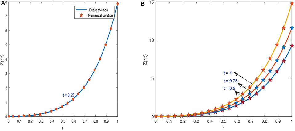
Figure 4. Approximate results of Example 5.2 at different time levels for α = 0.95, ν = 1, Δt = 0.0003, and h = 0.01. (A) For t = 0.25. (B) For t = 0.5, 0.75, and 1.

FIGURE 5

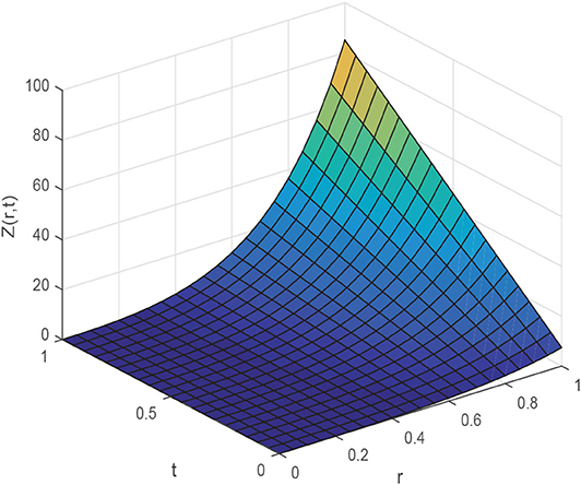
Figure 5. 3D preview of numerical solution of Example 5.2 for t ϵ [0, 1], α = 0.95, ν = 1, Δt = 0.0003, and h = 0.01.

TABLE 5

Table 5. Numerical results for Example 5.2.

TABLE 6

Table 6. Error norms for Example 5.2.

The approximate solution (2.3) can be written in piecewise form:

$\begin{array}{r}Z(r,t_n)={{\rm Y}}_{j-3}{\varphi }_{3,j-3}(r)+{{\rm Y}}_{j-2}{\varphi }_{3,j-2}(r)+{{\rm Y}}_{j-1}{\varphi }_{3,j-1}(r)\\ +{{\rm Y}}_j{\varphi }_{3,j}(r),r\in [r_j,r_{j+1}).& (5.5)\end{array}$

$\begin{array}{ll}{Z}_N(r,1)=\{\begin{array}{l}-5.4667r^3+0.9700r^2+14.08r+0.000033333,r\in [0,0.1),\\ -4.2667r^3+0.61r^2+14.116r-0.0011667,r\in [0.1,0.2),\\ -221.05r^3+130.68r^2-11.898r+1.7331,r\in [0.2,0.3),\\ -1.4667r^3-1.395r^2+14.614r-0.04415,r\in [0.3,0.4),\\ 5.35r^3-9.575r^2+17.887r-0.48042,r\in [0.4,0.5),\\ -1.6333r^3+0.9r^2+12.649r+0.3925,r\in [0.5,0.6),\\ 56.233r^3-103.26r^2+75.145r-12.107,r\in [0.6,0.7),\\ -104.25r^3+233.76r^2-160.77r+42.939,r\in [0.7,0.8),\\ 587.43r^3-1426.3r^2+1167.3r-311.2,r\in [0.8,0.9),\\ -1846.6r^3+5145.5r^2-4747.4r+1463.2,r\in [0.9,1).\end{array}& (5.6)\end{array}$

Example 5.3. For β = 2, the time fractional Fisher's equation becomes

$\begin{array}{ll}\frac{{\partial }^{\alpha }Z(r,t)}{\partial t^{\alpha }}-\nu \frac{{\partial }^{2}Z(r,t)}{\partial r^2}-Z(r,t)(1-Z^2(r,t))=f(r,t).& (5.7)\end{array}$

$\begin{array}{l}IC:Z(r,0)=0,0<r<1,\end{array}$

$\begin{array}{l}BCs:Z(0,t)=0,Z(1,t)=0,t\ge 0.\end{array}$

The source term

$\begin{array}{r}f(r,t)=\frac{24t^{4-\alpha }}{\Gamma (5-\alpha )}sin(2\pi r)\\ +4{\pi }^2{t}^{4}sin(2\pi r)-(t^{4}sin(2\pi r))(1-t^{4}sin(2\pi r)).\end{array}$

Exact solution for above conditions is

$\begin{array}{l}Z(r,t)=t^{4}sin(2\pi r).\end{array}$

Thus, the approximate solution (2.3) can be written in piecewise form:

$\begin{array}{r}Z(r,t_n)={{\rm Y}}_{j-3}{\varphi }_{3,j-3}(r)+{{\rm Y}}_{j-2}{\varphi }_{3,j-2}(r)\\ +{{\rm Y}}_{j-1}{\varphi }_{3,j-1}(r)+{{\rm Y}}_j{\varphi }_{3,j}(r),r\in [r_j,r_{j+1}).& (5.8)\end{array}$

$\begin{array}{ll}{Z}_N(r,1)=\{\begin{array}{l}-17815.0r^3+3562.9r^2+0.008r-23.753,r\in [0,0.1),\\ 5938.2r^3-3562.9r^2+712.59r-47.506,r\in [0.1,0.2),\\ 0.033333r^3-0.045r^2+0.0195r-0.00085,r\in [0.2,0.3),\\ -0.025r^2+0.0155r-0.00058333,r\in [0.3,0.4),\\ 1490.3r^3-1788.4r^2+715.36r-95.38,r\in [0.4,0.5),\\ -4470.7r^3+7153.2r^2-3755.4r+649.75,r\in [0.5,0.6),\\ 4470.8r^3-8941.7r^2+5901.5r-1281.6,r\in [0.6,0.7),\\ -1490.1r^3+3576.4r^2-2861.1r+762.98,r\in [0.7,0.8),\\ 0.016667r^3+0.005r^2-0.0425r+0.020917,r\in [0.8,0.9),\\ -0.033333r^3+0.14r^2-0.164r+0.057367,r\in [0.9,1).\end{array}& (5.9)\end{array}$

Figure 6A, displays the numerical and exact solution of Example 5.3 for t = 0.4, α = 0.96, h = 0.01 and Δt = 0.0001. The graphics illustrate that numerical and exact solutions are obviously shown to be indiscriminately comparable to one another. The effect of time concentrations t = 0.6, 0.8, and 1 is studied and presented in Figure 6B keeping other parameters constant. It can be seen from graphics that both solutions have symmetrical conduct and their corresponding numerical data are presented in Table 7, which demonstrates that both results are accurate and have negligible error. Figure 7 plots three-dimensional solution and results of error norms is given in Table 8.

FIGURE 6

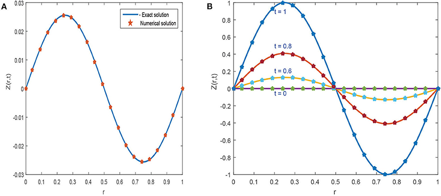
Figure 6. Numerical solution of Example 5.3 for variation in time at α = 0.96, ν = 1, h = 0.01, Δt = 0.0001, and β = 1. (A) For t = 0.25. (B) For t = 0, 0.5, 0.75, and 1.

TABLE 7

Table 7. Comparison of exact and numerical findings of Example 5.3 at various time stages.

FIGURE 7

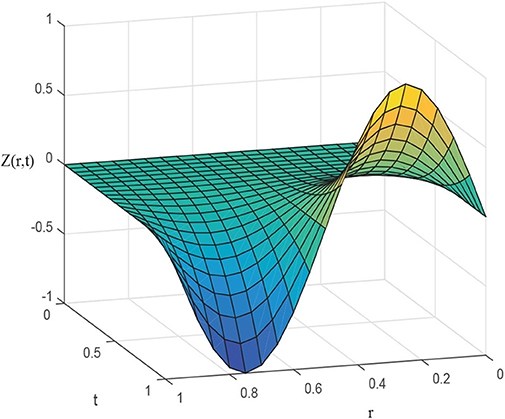
Figure 7. 3D image of approximate results of Example 5.3 for t ϵ [0, 1], α = 0.96, step size h = 0.01, Δt = 0.0001, and ν = 1.

TABLE 8

Table 8. Comparison of error norms of Example 5.3.

The influence of Brownian motion, i.e, α = 0.25, 0.75, on solution curve is displayed in Figure 8. The identical behavior of solution curves demonstrates that for smaller values of α, the solution profile is away from the exact result and as α → 1, the approximate and exact solution tends to overlap.

FIGURE 8

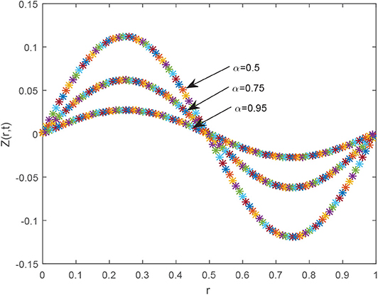
Figure 8. Approximate results of Example 5.3 for α = 0.5, 0.75 and 0.95, h = 0.01, Δt = 0.0001, and ν = 1.

Example 5.4. Fisher's equation with fractional order for β = 1 with f(r, t) = 0, is

$\begin{array}{ll}\frac{{\partial }^{\alpha }Z(r,t)}{\partial t^{\alpha }}-\nu \frac{{\partial }^{2}Z(r,t)}{\partial r^2}-Z(r,t)(1-Z(r,t))=f(r,t).& (5.10)\end{array}$

$\begin{array}{l}withIC:Z(r,0)={\sigma }^{*},0\le r\le 1.\end{array}$

The exact solution of the model for α = 1 is,

$Z(r,t)=\frac{exp(t){\sigma }^{*}}{1-{\sigma }^{*}+{\sigma }^{*}exp(t)}.$

The graphical illustration of exact and numerical solutions for Example 5.4 are shown in Figure 9. Figure 9A shows compatibility of exact and numerical results for h = 0.01, Δt = 0.02, α = 1, and σ^* = 0.25. The multiple curves for exact and numerical solutions for various values of σ^* = 0.5, 0.7, and 0.9 are shown in Figure 9B. The comparison of exact and approximate solutions acquired by the proposed scheme is expressed in Table 9. The tabular data demonstrate that both solutions are compatible with each other for various values of σ^*. Table 10 demonstrates the error norms.

FIGURE 9

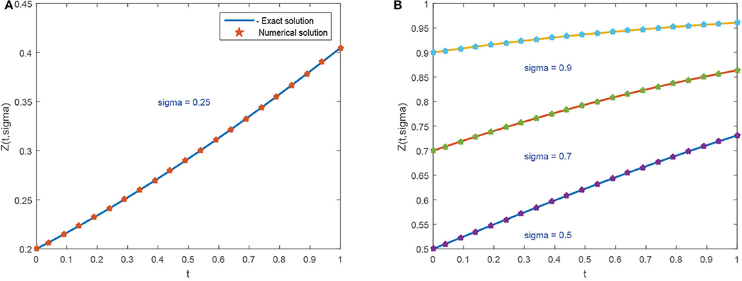
Figure 9. Numerical results of Example 5.4 for various values of σ^* and α = 1, Δt = 0.02, and h = 0.01. (A) For σ^* = 0.25. (B) For σ^* = 0.5, 0.7, and 0.9.

TABLE 9

Table 9. Exact and numerical results of Example 5.4 at different values of σ^*.

TABLE 10

Table 10. Comparison of error norms.

6. Concluding Remarks

In this study, cubic B-spline (CBS) scheme has been successfully implemented to acquire numerical solution of a time-fractional modified Fisher's equation for β = 2 and 3. The temporal derivative is discretized in the Caputo's sense by means of L1 formula, whereas CBS functions have been used for spatial derivative. The results acquired by the proposed scheme are presented in the form of tables and graphics. Following are the main outcomes of this study.

1. The existing Fisher's model has been modified by adding source term and by increasing integer power of non-linear term.

2. The influence of α parameter has been studied for different values and observed that, as the value of α increases gradually, the solution profile Z(r, t) tends toward exact solution. The numerical solution overlaps the exact solution as α approaches 1 as shown in figures.

3. The numerical behavior of the proposed model with different initial and boundary conditions has been observed at different time levels.

4. The comparison of exact and numerical results displayed in graphics reveals that both results show symmetrical behavior and their corresponding numerical data presented in tables clearly elaborate consistency of the results.

5. The results of the study regarding stability of the presented scheme show that proposed scheme is unconditionally stable.

Moreover, the accuracy and efficiency of the proposed scheme is quantified by computing error norms and the numerical results reflect that the proposed scheme is applicable for non-linear time fractional generalized Fisher's equation.

Author Contributions

All authors listed have made a substantial, direct and intellectual contribution to the work, and approved it for publication.

Conflict of Interest

The authors declare that the research was conducted in the absence of any commercial or financial relationships that could be construed as a potential conflict of interest.

The reviewer HS declared a past co-authorship with one of the authors JS to the handling editor.

References

1. Caputo M. Elasticita e Dissipazione. Bologna: Zanichelli (1969).

2. Miller KS, Ross B. An Introduction to Fractional Calculus and Fractional Differential Equations. New York, NY: Wiley (1993).

3. Liao SJ. Homotopy analysis method: a new analytic method for nonlinear problems. Appl Math Mech. (1998) 19:957–62. doi: 10.1007/BF02457955

CrossRef Full Text | Google Scholar

4. Scalar E, Gorenflo R, Mainardi F. Fractional calculus and continuous time finance. Phys A. (2000) 284:376–84. doi: 10.1016/S0378-4371(00)00255-7

CrossRef Full Text | Google Scholar

5. West BJ, Turalskal M, Grigolini P. Fractional calculus ties the microscopic and macroscopic scales of complex network dynamics. New J Phys. (2015) 17:045009. doi: 10.1088/1367-2630/17/4/045009

CrossRef Full Text | Google Scholar

6. Tarasov VE. Fractional vector calculus and fractional Maxwell's equations. Ann Phys. (2008) 323:2756–78. doi: 10.1016/j.aop.2008.04.005

CrossRef Full Text | Google Scholar

7. Rossa J, Villaverdeb AF, Bangab JR, Vazquezc S, Moranc F. A generalized Fisher equation and its utility in chemical kinetics. Proc Natl Acad Sci USA. (2010) 107:12777–81. doi: 10.1073/pnas.1008257107

PubMed Abstract | CrossRef Full Text | Google Scholar

8. Ammerman AJ, Cavalli-Sforza LL. The Neolithic Transition and the Genetics of Population in Europe. Princeton, NJ: Princeton University Press (1984).

PubMed Abstract | Google Scholar

9. Kerke VM. Results from variants of the Fisher equation in the study of epidemics and bacteria. Phys A. (2004) 342:242–8. doi: 10.1016/j.physa.2004.04.084

CrossRef Full Text | Google Scholar

10. Fisher RA. The wave of advance of advantageous genes. Ann Eugen. (1937) 7:355–69. doi: 10.1111/j.1469-1809.1937.tb02153.x

CrossRef Full Text | Google Scholar

11. Podlubny I. Fractional Differential Equations, Vol. 198 of Mathematics in Science and Engineering. San Diego, CA: Academic Press (1999).

12. Odibat Z. Approximation of fractional integrals and caputo fractional derivatives. Appl Math Comput. (2006) 178:527–33. doi: 10.1016/j.amc.2005.11.072

CrossRef Full Text | Google Scholar

13. Baleanu D, Diethelm K, Scalas E, Trujillo JJ. Fractional Calculus Models and Numerical Methods, Vol. 3 of Series on Complexity, Nonlinearity and Chaos. Singapore: World Scientific (2012).

Google Scholar

14. Baranwal VK, Pandey RK, Tripathi MP, Singh OP. An analytic algorithm for time fractional nonlinear reaction diffusion equation based on a new iterative method. Commun Nonlin Sci Numer Simul. (2012) 17:3906–21. doi: 10.1016/j.cnsns.2012.02.015

CrossRef Full Text | Google Scholar

15. Yang XJ, Machado JAT, Baleanu D. Anomalous diffusion models with general fractional derivatives within the kernels of the extended Mittag Leffler type functions. Rom Rep Phys. (2017) 69:120. Available online at:http://hdl.handle.net/20.500.12416/1850

Google Scholar

16. Yang XJ. Fractional derivatives of constant and variable orders applied to anomalous relaxation models in heat-transfer problems. Therm Sci. (2017) 21:116–71. doi: 10.2298/TSCI161216326Y

CrossRef Full Text

17. Yang XJ, Machado JAT, Cattani C, Gao F. On a fractal LC-electric circuit modeled by local fractional calculus. Commun Nonlinear Sci Numer Simul. (2017) 47:200–6. doi: 10.1016/j.cnsns.2016.11.017

CrossRef Full Text | Google Scholar

18. Alaattin E, Ucar Y, Yagmurlu N, Tasbozan O. A Galerkin finite element method to solve fractional diffusion and fractional diffusionwave equations. Math Model Anal. (2013) 18:260–73. doi: 10.3846/13926292.2013.783884

CrossRef Full Text | Google Scholar

19. Rubin SG, Graves RA. Cubic Spline Approximation for Problems in Fluid Mechanics. Washington, DC: NASA TR R-436 (1975).

Google Scholar

20. Wazwaz AM, Gorguis A. An analytic study of Fishers equation by using Adomian decomposition method. Appl Math Comput. (2004) 154:609–20. doi: 10.1016/S0096-3003(03)00738-0

CrossRef Full Text | Google Scholar

21. Abedle-Rady AS, Rida SZ, Arafa AAM, Adedl-Rahim HR. Approximate analytical solutions of the fractional nonlinear dispersive equations using homotopy perturbation Sumudu transform method. Int J Innov Sci Eng Technol. (2014) 19:257–67.

Google Scholar

22. Gupta AK, Ray SS. On the solutions of fractional Burgers Fisher and generalized Fishers equations using two reliable methods. Int J Math Math Sci. (2014) 2014:682910. doi: 10.1155/2014/682910

CrossRef Full Text | Google Scholar

23. Cherif MH, Belghaba K, Zaine D. Homotopy perturbation method for solving the fractional Fishers equation. Int J Anal Appl. (2016) 101:916.

Google Scholar

24. Khader MM, Saad KM. A numerical approach for solving the fractional Fisher equation using Chebyshev spectral collocation method. Chaos Solit Fract. (2018) 110:169177. doi: 10.1016/j.chaos.2018.03.018

CrossRef Full Text | Google Scholar

25. Rawashdeh MS. The fractional natural decomposition method: theories and applications. Math Methods Appl Sci. (2016) 40:2362–76. doi: 10.1002/mma.4144

CrossRef Full Text | Google Scholar

26. Singh H. An efficient computational method for the approximate solution of nonlinear Lane-Emden type equations arising in astrophysics. Astrophys Space Sci. (2018) 363:71. doi: 10.1007/s10509-018-3286-1

CrossRef Full Text | Google Scholar

27. Singh H. Approximate solution of fractional vibration equation using Jacobi polynomials. Appl Math Comput. (2018) 317:85–100. doi: 10.1016/j.amc.2017.08.057

CrossRef Full Text | Google Scholar

28. Majeed A, Piah ARM, Rafique M, Abdullah JY, Rajion ZA. NURBS curves with the application of multiple bones fracture reconstruction. Appl Math Comput. (2017) 315:70–84. doi: 10.1016/j.amc.2017.05.061

CrossRef Full Text | Google Scholar

29. Singh J, Kumar D, Swroop R. Numerical solution of timeand space-fractional coupled Burgers equations via homotopy algorithm. Alex Eng J. (2016) 552:1753–63. doi: 10.1016/j.aej.2016.03.028

CrossRef Full Text | Google Scholar

30. Najeeb AK, Ayaz F, Jin L, Ahmet Y. On approximate solutions for the time-fractional reaction-diffusion equation of Fisher type. Int J Phys Sci. (2011) 6:2483–96.

Google Scholar

31. Sayevand K, Yazdani A, Arjang F. Cubic B-spline collocation method and its application for anomalous fractional diffusion equations in transport dynamic systems. J Vib Control. (2016) 22:2173–86. doi: 10.1177/1077546316636282

CrossRef Full Text | Google Scholar

32. Dag I, Irk D, Saka B. A numerical solution of Burgers equation using cubic B-splines. Appl Math Comput. (2005) 163:199–211. doi: 10.1016/j.amc.2004.01.028

CrossRef Full Text | Google Scholar