
95% of researchers rate our articles as excellent or good
Learn more about the work of our research integrity team to safeguard the quality of each article we publish.
Find out more
ORIGINAL RESEARCH article
Front. Phys. , 03 July 2020
Sec. Social Physics
Volume 8 - 2020 | https://doi.org/10.3389/fphy.2020.00276
This article is part of the Research Topic Mathematical modelling of the pandemic of 2019 novel coronavirus (COVID-19): Patterns, Dynamics, Prediction, and Control View all 34 articles
The Gauss model for the time evolution of the first corona pandemic wave is rendered useful in the estimation of peak times, amount of required equipment, and the forecasting of fade out times. At the same time, it is probably the simplest analytically tractable model that allows us to quantitatively forecast the time evolution of infections and fatalities during a pandemic wave. In light of the various descriptors, such as doubling times and reproduction factors, currently in use to judge the lockdowns and other measures that aim to prevent spreading of the virus, we hereby provide both exact and simple approximate relationships between the two relevant parameters of the Gauss model (peak time and width), the transient behavior of two versions of doubling times, and three variants of reproduction factors, including basic reproduction numbers.
Recently [1], we demonstrated that the proposed [2–4] Gaussian time evolution for the daily number of cases (deaths or alternatively infections) at time t
provides a quantitatively correct description for the monitored rates in 25 different countries. Here, cmax is the maximum number of daily cases at peak time tmax and w a characteristic duration. The Gauss model (GM) is capable of reproducing reasonably well the monitored time evolution of the Covid-19 disease and, even more importantly, making realistic predictions for the future evolution of the first wave in different countries. An epidemologic foundation of the GM had been suggested by the agent-based model presented in Schüttler et al. [1]. The GM can furthermore be regarded as an approximant of the classical Susceptible-Infected-Recovered/Removed (SIR) model [5, 6] in the limit of large inverse basic reproduction numbers [7]. From a mathematical viewpoint, a sigmoidal time evolution involving a polynomial in the exponent of an exponential can be Taylor expanded about the maximum; the GM corresponds to the lowest non-trivial order of a Taylor expansion.
Values for the parameters of the GM had been extracted by fitting the natural logarithm of the monitored rates with
which is a polynomial of second order in t, to derive the best fit values and their confidence errors of the three parameters cmax, w, and tmax. These parameters are country specific and reflect the regional differences in treatment, geographical, political, socioeconomic situations, available equipment, etc. If this fitting and parameter determination is done during the early stage of the pandemic wave, the GM makes predictions for the later time evolution of the wave.
The starting time of the outbreak, t0 can be defined by the first occurrence of a case, c(t0) = 1, and is thus known from the parameters of the Gaussian. Inverting c(t0) = 1 readily yields , or
To simplify notation, besides absolute time t, we introduce two more times. First, there is the time relative to the peak time, denoted by
so that negative (positive) Δ correspond to times before (after) the peak time. Second, there is the dimensionless time x = −Δ/w. As time unit we choose days throughout, so that Δ = +2 corresponds to 2 days after peak time, and w is also given in units of days; meanwhile, c is a dimensionless number of cases, usually renamed as d or i if we specialize to deaths or infections. The three parameters of the GM are related but not identical for deaths and infections, as discussed earlier [1]. The related—to Equation (3)—starting time
is negative, is positive, and |Δ0| is the number of days between outbreak and climax of the first pandemic wave. All properties derived for the GM must therefore depend on w, cmax, and x or, alternatively, Δ, where Δ ∈ [Δ0, ∞].
Often monitored data are reported in terms of doubling times and effective reproduction factors. These are also important indicators for the future temporal evolution of the disease, especially if no functional form for the case temporal evolution, such as the GM (2), is adopted. However, there are differently defined doubling times as well as reproduction factors in use. It is the purpose of this manuscript to discuss in detail the properties of differently defined doubling times and the differently defined reproduction factors, their mutual relations to each other, and their temporal behavior for the GM.
As before [2], we consider the relative change of the daily number of cases for the GM
where the prime denotes a derivative with respect to time t, c′(t) = dc(t)/dt. The monitored data are often given in terms of the instantaneous doubling time d of the corresponding exponential functions at any time for the daily number of cases
with the obvious properties ca(t + d) = 2ca(t). With these corresponding exponential functions, we obtain for the relative changes in the daily rate
Equating the two results, (6) and (8), leads to the time-dependent differential Gaussian doubling time
Apart from the changed notation, these differential Gaussian doubling times agree with the earlier derived Equation (5) in Schlickeiser and Schlickeiser [2]. The differential doubling time is positive for times earlier than the peak time, Δ < 0, and monotonically increases over time until it diverges as it approaches Δ = 0. For later times Δ > 0 the doubling time is formally negatively valued but corresponds to positively valued half-life approaching 0 for Δ → ∞. Because of the divergence at Δ = 0 and its negative value for Δ > 0, daily doubling times are of limited use only before the peak time of the outburst; instead, in the public discussion, cumulative doubling times are often preferred, which we discuss in the next subsection. Apart from the time Δ relative to the peak time, the daily instantaneous doubling time (9) is determined by the width w of the Gaussian time evolution function (1). Figure 1 displays the distribution of widths w determined by the best fit of the GM to the death rates in 67 countries, indicating that w ∈ [12, 34] with a mean value of 18.96.
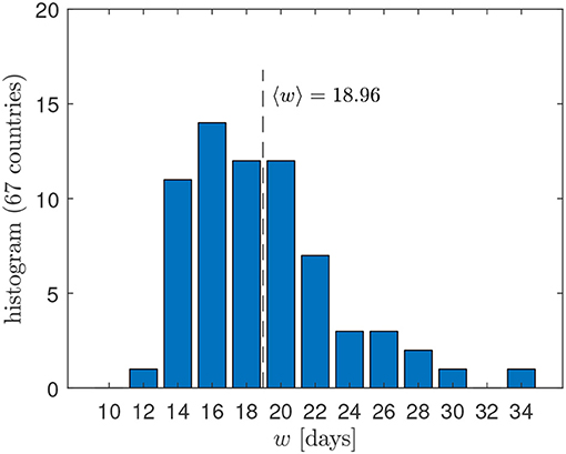
Figure 1. Distribution of widths w obtained by the best fit of the GM to the death rates in 67 different countries [8].
We emphasize that, at early times t of the time evolution, characterized by t0 ≤ t ≪ tmax Or, equivalently, Δ0 ≤ Δ ≪ 0, the Gaussian time evolution function (1) approaches an exponential distribution because the exponent becomes linear in t and thus also linear in Δ. At such early times, the time relative to the peak time (4) is Δ0, so that the differential Gaussian doubling time (8) approaches the constant
characterizing the initial, exponential growth.
Instead of defining doubling times with daily number of cases one may also define them with the cumulative case rate. From Equations (1) and (4), one has for the corresponding cumulative number of cases at time t
respectively, in terms of the error function, where
denotes the total number of cases. Such values for fatalities, Dtot, and infections, Itot, relevant for the first pandemic wave of the Sars-Cov-2 virus were obtained in Schüttler et al. [1]. With the cumulative numbers (11), we found for the respective relative change
Equating these results again with Equation (8) for the corresponding exponential function1 leads to the time-dependent cumulative Gaussian doubling times
where abbreviates the numerical prefactor. Using the identities 1 + erf(x) = 1 − erf(−x) = erfc(−x) in terms of the complimentary error function, we express Equation (14) as
with the function
As opposed to doubling times calculated from daily rates, doubling times derived from cumulative numbers are strictly positive, monotonically increase in the course of time, but never diverge, and remain finite at Δ = 0. Because x = −Δ/w, the argument x of F(x) is positive before and negative after the peak time.
In Appendix 1, we investigate the properties of the function F(x) and its approximations. It is convenient to consider times t before and after the peak time tmax, i.e., negative and positive Δ. We consider each in turn.
With the approximation (50) from the Appendix we obtain for the cumulative doubling time (15) at times t ≤ tmax
where Δ = t − tmax is negative, and χ/3 ≃ 0.205. Dbefore(t) continuously increases with time until it reaches Dmax (21) at peak time. At early times of the time evolution t ≪ tmax, not only d but also the cumulative Gaussian doubling time (15) or (17) approaches the constant
reflecting again the result that, at an early time, the Gaussian time distribution function (1) approaches an exponential distribution function with the constant doubling time (10) so that also the cumulative distribution function initially displays an exponential behavior. The ratio of the two, differential (10) and cumulative (18), limits is given by
with F from definition (16).
Here, we use the property (46) and the approximation (50) to obtain the cumulative doubling time (15)
with 2χ ≃ 1.229 and where we can make use of Dbefore(t) from Equation (17) because it was written for this purpose in terms of |Δ|. However, this Gaussian cumulative doubling time Dafter(t) for times t > tmax is only a formal indicator for the decreasing slope of the cumulative rate C(t). As the cumulative rate (11) indicates, at the peak times tmax, it has the value C(tmax) = Ctot/2, so that, for any times greater than tmax, the cumulative rates can no longer double. This implies that only the maximal cumulative doubling time
has a real physical meaning. In Figure 2, we calculate the Gaussian daily instantaneous and cumulative doubling times as a function of the time Δ relative to the peak time for three values of the Gaussian width w = 10, 15, 20. At times below the peak time Δ < 0, the two doubling times have a similar behavior. As Δ → 0 the instantaneous doubling times becomes infinitely large, whereas the cumulative doubling times approaches large but finite values. However, as noted before, for times Δ > 0, the Gaussian cumulative doubling time Dafter(t) is only a formal indicator for the decreasing slope of the cumulative rate C(t) that can no longer double at any times larger than tmax.
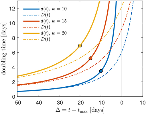
Figure 2. Comparison of the daily instantaneous (d) and cumulative (D) doubling times as a function of the time Δ relative to the peak time for three values of the Gaussian width w = 10, 15, 20. The circles mark Δ0 for cmax = 1, cf. Equation (5): the GM should not be used at times smaller than Δ0.
Nevertheless, cumulative doubling times are issued by health agencies, such as the Robert-Koch-Institut, to the public also at times after the peak time: they can cause much confusion among the public, as they suggest by their name that the cumulative case rate can still double beyond its 50% value, although this is no longer possible. Instead, one should refer to the effective reproduction factor at this stage of the wave time evolution, which we discuss next.
In epidemiology, the basic reproduction number R0 (sometimes called basic reproductive ratio, or incorrectly basic reproductive rate) of an infection can be thought of as the expected number of cases directly generated by one case in a population where all individuals are susceptible to infection [9, 10]. The definition describes the state where no other individuals are infected or immunized (naturally or through vaccination). Some definitions, such as that of the Australian Department of Health, add absence of any deliberate intervention in disease transmission. Within this manuscript, R0 is thus identical to the R(t) at the starting time of the outbreak, i.e., R(t0) = R0.
The basic reproduction number R0 is not to be confused with the effective, time-dependent reproduction factor R(t); this is the number of cases generated in the current state of a population, which does not have to be the uninfected state. By definition, R0 cannot be modified through vaccination campaigns. Also, it is important to note that R0 is a dimensionless number and not a rate, which would have units of time like doubling time [9, 10]. Still, the basic reproduction number R0 will be seen to correspond to R(t) evaluated at time t0.
The definition of the effective reproduction factor R(t) according to [11, 12] is
where c(t) is the number of daily cases (deaths or infections, usually the reproduction factor is obtained from the reported number of daily infections) at time t, and W(s) denotes the serial interval distribution [13]. This distribution describes the probability for the time lag between a person's infection and the subsequent transmission of the virus to a second person, and it is known to have an effect on the reproduction factor [14]. The discrete sum in Equation (22) starts from zero rather than unity as in references [11, 12], because W(0) = 0 and because we are here interested in the continuous generalization of Equation (22).
Written in terms of integrals, Equation (22) corresponds to [15]
while the serial interval distribution W(s) has to be properly normalized to unity, i.e.,
This normalization is required in order to ensure, according to Equation (23), that a constant stationary c(t) implies R(t) = 1. Note that in Scirea et al. [12] they wrote E[c(t)] instead of c(t) on the left hand side of Equation (22), where E[] signals that c(t) is an expectation value involving the serial distribution. Here, we consider c(t) to be defined by Equation (22) so that c(t) can be evaluated for the GM via Equation (1).
In the following we investigate two different choices of the serial interval distribution evaluated for the GM: (i) the gamma distribution, as in previous studies [11, 12], and (ii) the analytically simpler box-shaped serial interval distribution. We consider each in turn.
Here, the serial interval distribution W(s) is taken to be the gamma distribution [16]
with the shape parameters α = 2.785 and β = α/6.5 that seem to represent the distribution used in reference [11]. They used another convention but mentioned the mean value 〈s〉 = 6.5 and provided an excel file. The mean value of this distribution (25) is
For the specified parameters, the distribution (25) is very well-approximated (absolute error < 0.006) by the slightly more convenient and, again, properly normalized distribution
yielding a mean value 〈s〉 = 3/b. We adopt b = 4/9 = 0.444, leading to the mean 〈s〉 = 27/4 = 6.75 days, which is very close to the earlier chosen mean [11] 〈s〉 = 6.5 days. In Figure 3 we compare the approximation (27) with the discrete distribution used in reference [11] (black circles) during all their calculations.
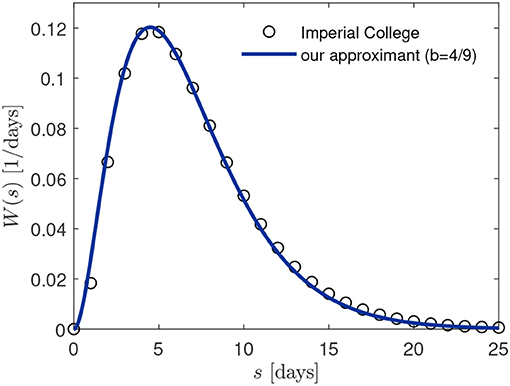
Figure 3. Comparison of serial interval distribution W(s) employed in [11, 12] (black circles) and our approximant (27) with b = 4/9.
Here, we use the known for the GM (1). As for the doubling times, R(t) does not depend on the magnitude cmax and absolute time t but can be expressed in terms of the relative time Δ = t − tmax and w. With c(t − s) ~ exp[−(Δ − s)2/w2], And, with W(s) from (27), we can thus proceed and calculate R(t) analytically as
involving the time-dependent integral
where and . To this end, it turns out convenient to switch to dimensionless times. We have already introduced x, and we now introduce a characteristic xc
and the dimensionless, time-dependent distance X between x and xc via
As shown in Appendix 2, the integral (29) can be evaluated analytically to yield
with the function F given by (16). Consequently, the effective reproduction factor (28) becomes (Figure 5)
in terms of x and the negatively valued xc, where we recall that x = (tmax − t)/w = −Δ/w carries the dependency on time t. The effective reproduction factor approaches the basic reproduction number R0 at small times and assumes the important value R(t) = 1 roughly 4 days after peak time at Δ≈4, as Figure 5 indicates. It is not difficult to show that this Δ asymptotically approaches 2/b = 9/2 = 4.5 days for large w (Appendix 4.1).
While the basic reproduction number R0 for the GM can be read off from (33) upon replacing x by (shown in Figure 4), it is insightful to make the connection between R0 and the early doubling time , according to (10). As the Gaussian time distribution is exponential at early times, in the vicinity of t ≃ t0, we can insert the exponential growth (7) into definition (23) with the gamma-shaped serial distribution W(s). This yields a time-independent constant effective reproduction factor
where b = 4/9 and where we have also mentioned its appearance in terms of dimensionless x0 and xc. Since d0 is positive, the exponential effective reproduction factor at time t0 (34) is greater than unity and provides an approximation for the exact one (Figure 4). It is worthwhile to mention that the same result is obtained without assuming a purely exponential growth but instead by starting from (33) and assuming x0 ≫ xc + 1 (for a proof see Appendix 3.1). For a model with purely exponential growth characterized by a single doubling time d0, Equation (34) provides the exact relationship between doubling time and basic reproduction number and R(t) = R0.
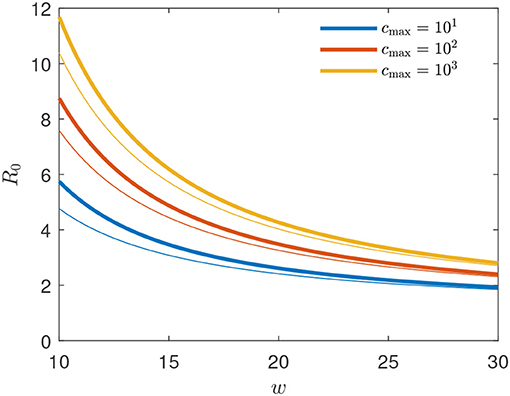
Figure 4. Basic reproduction number R0 = R(t0) for the GM as function of peak width w for several peak heights cmax (thick solid lines). For comparison, the thin lines show the approximant (34). The exact R0 is given by (33) evaluated at .
Adopting b = 4/9 and w = 20 and thus xc = −40/9 according to (30), provides for the number (34)
yielding the estimates 4.77, 4.03, and 3.26 for , 103, and 102, respectively, close to the exact values given by R(t0) from Equation (33). The values of Δ0 and R0 for different values of the width w and cmax = 1 are marked by circles in Figure 5.
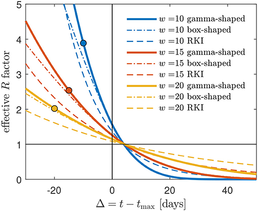
Figure 5. Gamma-shaped R(t) (33) compared with the approximate R(t) (37) (red, dashed), using a box-shaped serial interval distribution W(s), and the RKI formula (41). Cases shown are w = 10, w = 15, and w = 20. Deviations are most pronounced and significant for the smallest w = 10. The R(t) curves terminate at t = t0 corresponding to Δ = Δ0, see (5). The circles mark Δ0 for cmax = 1.
Here, we address the question on how relevant it is to take into account the correct shape of serial interval distribution when calculating R(t) via (23).
If we consider W(s) to be approximated by a constant independent on s on the interval s ∈ [0, smax], and consider it to be zero otherwise, the requirement of its proper normalization (24) and unchanged mean value 〈s〉 = 6.5 compared with the unapproximated W(s) from (25) yields
with the two-sided Heaviside Θ(x, A, B) = 1 for A ≤ x ≤ B and Θ(x) = 0 otherwise.
With the Gaussian evolution (1) and the box-shaped serial interval distribution (36) inserted, we obtain with the help of (23)
plotted in Figure 5. As is visible, the box-shaped W(s) can serve as a good approximation as long as w is sufficiently large, and Δ not too small. It crosses the R = 1 line roughly 4 days after peak time and shares this feature with the case of the gamma-shaped serial distribution. This aspect is worked out in detail in Appendix 4. Starting from R(t) = 1 with R(t) from (37), the exact asymptotic value is t = tmax + (smax/3) days (proof in Appendix 4.2).
The basic reproduction number is given by R(t0), which amounts to replacing Δ by Δ0 in (37). As before, it is useful to consider a regime of exponential growth to come up with a simple approximant for R0, now using a box-shaped W(s). Inserting the exponential time evolution (7) with constant d0 and the box-shaped serial interval distribution (36) into Equation (23), we obtain the time-independent constant effective box reproduction factor that serves an approximant for R0,
which is always greater than unity for positive d0. Since smax ln 2 ≈ 9 days, we thus have
as long as d0 < 9 days, which is the usual scenario (Figure 2). As already mentioned, the box-shaped serial interval distribution is better not used to estimate R0. It significantly underestimates the R0 obtained with the gamma serial distribution.
The RKI estimates an effective reproduction factor from the daily measured number i(t) of people that have been recognized to be infected as follows
Here, we again use the continuous version. Because measured data is not available for the future and is not sufficiently reliable if collected within the time frame of a few days, the RKI estimates R(t) for a time t that lies one 8 days the past. A connection between (40) and the true effective reproduction number is based on the assumption that the true number of cases is proportional to the measured ones at any time.
Using the GM instead of measured numbers for i(t), the estimated true number of cases (deaths or infections) in Equation (40) yields
shown in Figure 5. With (41) at hand, one can predict the RKI version of R(t) at all times during the first wave of a pandemic. A time of interest is when R drops below unity. Equation (41) readily yields for Δ = 4, with erf(0) = 0,
in agreement with Figure 5. It is this feature of the RKI, shared with the R(t) for the gamma serial distribution, that may have given rise to the choice of the interval length of 4 days in its definition. Figure 6 shows, for typical values between w = 15 and w = 20 days, how the R(t) calculated via the box-shaped W(s), and even more the RKI value, overestimate the R(t) at times beyond peak time.
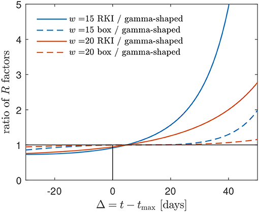
Figure 6. The R(t) factors obtained using (i) the box-shaped W(s) and (ii) the RKI formula greatly overestimate the R(t) using a gamma-shaped serial interval distribution at times beyond the peak time. Alternative representation of the data already shown in Figure 5. The mismatch increases with decreasing w. A typical w is in the range between 15 and 20 days for most countries [1] (cf. Figure 1).
As in previous sections, we can read off the basic reproduction number R0 upon inserting Δ0 instead of Δ into the expression for R(t) (41), and we can provide an approximate expression for R0 upon considering purely exponential, initial growth. Following this route, inserting monoexponential into (40) yields
While the two approximants (34) and (43) for basic reproduction numbers look different at first glance, they are quantitatively very similar: for d0 = 1, for example, (34) evaluates to 16.77, while (43) equals 16.0. Likewise, for d0 = 2 (34) evaluates to 5.64, while (43) equals 4.0. In the limit of d0 → ∞, both versions yield R0 = 1. The RKI version generally underestimates R0, as given by (34), but by no more than about 35%.
The Gauss model for the time evolution of the first corona pandemic wave rendered useful in the estimation of peak times, amount of required equipment, and the forecasting of fade out times. At the same time, it is probably the simplest analytically tractable model that allows to quantitatively forecast the time evolution of infections and fatalities during a pandemic wave. For these descriptions and forecasts, various descriptors, such as doubling times and reproduction factors are currently used in order to judge lockdowns and other non-pharmaceutical measures that aim to prevent spreading of the virus. As different definitions of doubling times and reproduction factors and numbers are used in the literature, we have provided in this manuscript both exact and simple approximate relationships between the two relevant parameters of the Gauss model (peak time tmax and width w) as well as the transient behavior of two versions of doubling times and three variants of reproduction factors R(t), including basic reproduction numbers R0.
Regarding doubling times, we considered both differential doubling times calculated from the daily number of cases and cumulative doubling times calculated from the cumulative case rates. The former differential doubling time is positive for times earlier than the peak time and monotonically increases in the course of time until it diverges as it approaches the peak time. For later times after the peak time, the differential doubling time is formally negatively valued but corresponds to positively valued half-life. Because of the divergence at the peak time and its negative value beyond, differential doubling times are of limited use only before the peak time of the outburst; instead, in the public discussion, cumulative doubling times are often preferred.
As opposed to doubling times calculated from daily rates, doubling times derived from cumulative numbers of cases are strictly positive, monotonically increase in the course of time, but never diverge, and remain finite at and after the peak time. At times below the peak time, the two doubling times have a similar behavior. However, the Gaussian cumulative doubling time for times after the peak time is only a formal indicator for the decreasing slope of the cumulative rate of cases. The Gaussian cumulative rate at the peak time attains exactly 50% of its maximum value after infinite time so that, for any times larger than the peak time, the cumulative rates can no longer double. This implies that only the maximal cumulative doubling time 0.614w has a real physical meaning.
Because of these two drawbacks of differential and cumulative doubling times in characterizing the time evolution of the corona wave after its peak time, health agencies, such as the German Robert-Koch-Institute (RKI) instead refer to the effective reproduction factor of the disease R(t), which is the number of cases infected in the current state of a population by a single individual infected person. As long as this factor remains smaller than unity the number of infections per day decreases with time. The effective reproduction factor is calculated from an integral involving the serial interval distribution W(s) normalized to unity and the differential case time distribution. For the GM, the latter is known analytically, and we investigated three different effective Gaussian reproduction factors: (i) the first is calculated with a gamma-function type serial interval distribution, (ii) the second is calculated with a flat box-shaped serial interval distribution, and (iii) the third, referred to as RKI estimate, involves the ratio of two consecutive 4-days time intervals of the monitored daily cases.
All three discussed effective reproduction factors, calculated with the GM, decrease from the base reproduction number R0 at the beginning of the pandemic wave to very small values at times much larger than the peak time. They all cross the critical value R = 1 about 4 days after the peak times. As the approximated RKI estimate for Germany still, many weeks after the peak times of the infection and death rates, occasionally indicates effective reproduction factors greater than unity, this has to be due to short intraday fluctuations of the rates. Such factors greater unity at late times after the peak time contradict the much smaller (below unity) effective reproduction factors from the GM, as we have demonstrated by Figure 6. As the GM provides reasonable descriptions of the overall temporal evolution of the infection and death rates in Germany, we have to conclude that the present RKI estimate of the effective reproduction factor overestimates the influence of short intraday fluctuations in the reported cases.
All datasets presented in this study are included in the article/Supplementary Material.
All authors listed have made a substantial, direct and intellectual contribution to the work, and approved it for publication.
The authors declare that the research was conducted in the absence of any commercial or financial relationships that could be construed as a potential conflict of interest.
The Supplementary Material for this article can be found online at: https://www.frontiersin.org/articles/10.3389/fphy.2020.00276/full#supplementary-material
1. ^We note that for a daily exponential rate in time also the cumulative number will be an exponential function in time.
1. Schüttler J, Schlickeiser R, Schlickeiser F, Kröger M. Covid-19 predictions using a Gauss model, based on data from April 2. Physics. (2020) 2:197–212. doi: 10.3390/physics2020013
2. Schlickeiser R, Schlickeiser F. A Gaussian model for the time development of the Sars-Cov-2 corona pandemic disease. Predictions for Germany made on March 30, 2020. Physics. (2020) 2:164–70. doi: 10.3390/physics2020010
3. Ciufolini I, Paolozzi A. Mathematical prediction of the time evolution of the COVID-19 pandemic in Italy by a Gauss error function and Monte Carlo simulations. Eur Phys J Plus. (2020) 135:355. doi: 10.1140/epjp/s13360-020-00383-y
4. Lixiang L, Yang Z, Dang Z, Meng C, Huang J, Meng H, et al. Propagation analysis and prediction of the COVID-19. Infect Dis Model. (2020) 5:282–92. doi: 10.1016/j.idm.2020.03.002
5. Kermack WO, McKendrick AG. A contribution to the mathematical theory of epidemics. Proc R Soc A. (1927) 115:700–21. doi: 10.1098/rspa.1927.0118
6. Kendall DG. Deterministic and stochastic epidemics in closed populations. In: Proceedings of the Third Berkeley Symposium on Mathematical Statistics and Probability. Vol. 4. Berkeley, CA: University of California Press (1956). p. 149–65.
7. Barmparis GD, Tsironis GP. Estimating the infection horizon of COVID-19 in eight countries with a data-driven approach. Chaos Solit Fract. (2020) 135:109842. doi: 10.1016/j.chaos.2020.109842
8. Kröger M. COVID-19 Real Time Statistics & Extrapolation Using the Gauss Model (GM). (2020). Available online at: https://www.complexfluids.ethz.ch/corona (accessed May 16, 2020).
10. Fraser C, Donnelly CA, Cauchemez S. Pandemic potential of a strain of influenza A (H1N1): early findings. Science. (2009) 324:1557–61. doi: 10.1126/science.1176062
11. Flaxman S, Mishra S, Gandy A, Unwin H, Mellan TA, Coupland H, et al. Estimating the effects of nonpharmaceutical interventions on COVID-19 in Europe. Nature. (2020). doi: 10.1038/s41586-020-2405-7. [Epub ahead of print].
12. Scirea J, Sarah N, Vaughana TG, Brupbacher G, Fuchs S, Sommer J, et al. Reproductive number of the COVID-19 epidemic in Switzerland with a focus on the Cantons of Basel-Stadt and Basel-Landschaft. Swiss Med Wkly. (2020) 150:w20271. doi: 10.4414/smw.2020.20271
13. Nishiura H, Linton NM, Akhmetzhanov AR. Serial interval of novel coronavirus (COVID-19) infections. Int J Infect Dis. (2020) 93:284–6. doi: 10.1016/j.ijid.2020.02.060
14. Wallinga J, Lipsitch M. How generation intervals shape the relationship between growth rates and reproductive numbers. Proc R Soc B. (2007) 274:599–604. doi: 10.1098/rspb.2006.3754
15. Fraser C. Estimating individual and household reproduction numbers in an emerging epidemic. PLoS ONE. (2007) 2:e758. doi: 10.1371/journal.pone.0000758
Keywords: coronavirus, statistical analysis, extrapolation, parameter estimation, pandemic spreading
Citation: Kröger M and Schlickeiser R (2020) Gaussian Doubling Times and Reproduction Factors of the COVID-19 Pandemic Disease. Front. Phys. 8:276. doi: 10.3389/fphy.2020.00276
Received: 16 May 2020; Accepted: 22 June 2020;
Published: 03 July 2020.
Edited by:
Aristides Moustakas, University of Crete, GreeceReviewed by:
Giorgos P. Tsironis, University of Crete, GreeceCopyright © 2020 Kröger and Schlickeiser. This is an open-access article distributed under the terms of the Creative Commons Attribution License (CC BY). The use, distribution or reproduction in other forums is permitted, provided the original author(s) and the copyright owner(s) are credited and that the original publication in this journal is cited, in accordance with accepted academic practice. No use, distribution or reproduction is permitted which does not comply with these terms.
*Correspondence: Martin Kröger, bWtAbWF0LmV0aHouY2g=; Reinhard Schlickeiser, cnNjaEB0cDQucnVoci11bmktYm9jaHVtLmRl
Disclaimer: All claims expressed in this article are solely those of the authors and do not necessarily represent those of their affiliated organizations, or those of the publisher, the editors and the reviewers. Any product that may be evaluated in this article or claim that may be made by its manufacturer is not guaranteed or endorsed by the publisher.
Research integrity at Frontiers

Learn more about the work of our research integrity team to safeguard the quality of each article we publish.