The Forest Fire Model: The Subtleties of Criticality and Scale Invariance

Amongst the numerous models introduced with SOC, the Forest Fire Model (FFM) is particularly attractive for its close relationship to stochastic spreading, which is central to the study of systems as diverse as epidemics, rumors, or indeed, fires. However, since its introduction, the nature of the model's scale invariance has been controversial, and the lack of scaling observed in many studies diminished its theoretical attractiveness. In this study, we analyse the behavior of the tree density, the average cluster size and the largest cluster and show that the model could be of high practical relevance for the activation dynamics seen in brain and rain studies. From this perspective, its peculiar scaling properties should be regarded as an asset rather than a limitation.

1. Introduction

Soon after the seminal paper introducing Self-Organised Criticality (SOC) [1], it was suggested that examples of SOC could include models describing the spread of activation in a manner reminiscent of forest fires or infectious diseases. The degree to which these models were examples of scale invariance and criticality instantly became a subject of intense debate, see, e.g., [2, 3]. Despite the controversy and indications that the Drossel-Schwabl Forest Fire Model [2] lacks scale invariance [4, 5], the dynamics of the model is of a type that seems of direct relevance to many real systems such as the brain [6] and precipitation [7]. So if for no other reason, it is still worthwhile to develop a better understanding of the behavior generated by this kind of stochastic spreading and relaxation dynamics and to develop ways to probe the dynamics which can be applied to data from real systems.

SOC focuses on criticality in the sense of equilibrium statistical mechanics, and for this reason, one typically looks for scale invariance and dynamics that can tune sharply to a critical point. Conversely, broad crossover behavior is not seen as properly belonging to the SOC paradigm. However, the relevance of a theoretical scientific framework is, in the end, determined by how useful it is for the description and analysis of real systems. Seen from this perspective, it is of importance to bear in mind that exact fine-tuning to a completely scale-invariant state is not always observed in systems that exhibit SOC-like behavior. This is demonstrated, e.g., by the studies of the size distribution of rain showers [7], and the bursts of brain activity measured during fMRI scans [6]. Indeed, neither study finds sharp critical behavior but, despite the systems being of totally different microscopic nature, both identify similar indications of critical behavior in terms of approximate power laws and even features reminiscent of peaked, or perhaps diverging, fluctuations or susceptibilities. Moreover, both studies find that the dynamics pulls the systems into a crossover region of large fluctuations within which one most frequently finds configurations to reside. In other words, in both cases, the distribution of residence times, i.e., the amount of time spent at a certain value of the control parameter, is found to exhibit a broad peak centered about what appears to be a critical-like value of the control parameter. From our experience with equilibrium critical phenomena, one would expect a broad peak for small system sizes only, and that the width of the peak will shrink with increasing system size. Therefore, for systems as big as the atmosphere or with as many components as the brain, broad peaks would not be expected.

The experimental observations in [6, 7] suggest that the dynamics couples the control parameter to the fluctuations in a way that makes the system move around in a critical region, rather than tuning to a critical point. This is similar to suggestions previously put forward, such as [8, 9]. Intuitively, one may imagine something like the following in the case of precipitation: nucleation of drops can happen at a particular value of the vapor content. The vapor in the atmosphere over the ocean gradually builds up toward that value, and sometimes overshooting may even occur before nucleation is seeded. When precipitation events occur, a significant amount of vapor is removed from the atmosphere, and one observes oscillations between subcritical and supercritical regions. For some reason, the coupling between the driving (vapor formation) and the response (precipitation) produces such large fluctuations that a precise tuning to the critical value of the control parameter is excluded. A parallel situation may take place in the brain as neurones have to go through a refractory period before they are able to fire again after discharge.

A link between the behavior observed in brain activity and rainfalls [6, 7] and the Forest Fire Model was already suggested in [10]. Inspired by these studies, we analyse in detail the residence time distribution (which corresponds to the tree density distribution in the FFM) and its relationship to the order parameters used in standard percolation [11] and the brain study [6], namely the average cluster size and the normalized size of the largest cluster. We find that there is indeed a critical-like region where the fluctuations peak up and where the system seems to spend most of the time, exactly like in the brain and rain observations. Furthermore, analyzing the distribution of the non-normalized largest cluster, we find that it displays scale invariance for our reachable system sizes and that its first moment seemingly grows superlinearly with the activity θ, in a way that reminds the superlinear growth of the instantaneous correlation length observed in [12].

2. Model Description

As reported in [3], the original forest fire model proposed in [13] was revised in [2] and became known in the literature as the Drossel-Schwabl Forest Fire Model (DS-FFM), despite the resulting model coinciding with the one introduced a few years before in [14] as Self-organised percolation. In the following, we will analyse the model proposed in [2, 14] and refer to it simply as forest fire model (FFM). The FFM consists of a dissipative dynamic that involves the occupation of empty sites (planting of trees) and the removing of clusters of trees (burning of a forest). In the following, we will restrict our simulations to a two-dimensional square grid with periodic boundary conditions and side length L. Our implementation follows [4, 10, 12, 15–17], and is summarized by the following pseudocode [10]. An efficient implementation of the FFM can be found at [18].

ALGORITHM 1

Algorithm 1: Forest Fire Model

Clusters are computed considering 4 neighbors for each site (2 horizontal and 2 vertical). In order to avoid finite-size effects, θ has to be tuned, taking into account the system size L². In our simulations, we keep fixed the ratio $k=\frac{\theta }{L^2}$ as in [12]. The great majority of the simulations are done at k = 10⁻³, but we also present results for smaller values of k in Figures 3, 10. Since the model is known for taking a long time to thermalize, we performed 5 · 10⁶ burning steps for thermalization and 10⁶ to collect the statistics as in [4]. The only exception is for the heatmaps in Figures 7, 8, where 10⁷ datapoints were used to produce the statistics.

3. Results

3.1. The Distribution of Densities

To compute the distribution of the densities P(ρ), we assign one spatially averaged density ρ to each generated configuration and sample the distribution over the ensemble. In this way, we obtain an object that is equivalent to the distribution of residence times in [6, 7]. In the early studies of the FFM, the average density of trees 〈ρ〉 was assumed to behave as

$\begin{array}{ll}\langle \rho \rangle ={\rho }_{\infty }-a{\theta }^{-b}& (1)\end{array}$

Where ρ_∞ is the supposedly asymptotic density of trees and a and b are two constants. The value of the power was estimated as b = 0.47 in [19, 20] and b = 0.5 in [15]. However, it was noted in [5] that for θ ≳ 10⁴ the average density starts to deviate dramatically from the estimates made at lower values, ending up to be more than 100 standard deviations higher than the expected value for θ ~ 10⁵, and seemingly growing as a pure power law for θ ≳ 10⁴. Assuming that the power law behavior holds asymptotically in θ, it was estimated in [5] that the tree density would reach the percolation density (ρ_p ≃ 0.5927…) for θ ~ 10⁴⁰.

To avoid finite-size effects, in [5] the values of θ and L were chosen as follows: for every value of θ, several simulations were carried out at different system sizes, and it was verified that the distribution of the rms radius, cluster sizes, and burning time were independent of L. The distribution of densities, on the other hand, depends strongly on the system size. For a fixed value of θ, increasing the system size would make the variance of the distribution decrease as L⁻² in the absence of finite size effects [4]. Conversely, fixing L and increasing θ would lead to an increase in the standard deviation and 〈ρ〉, as can be seen in Figure 1. In the following, we will focus our attention on the behavior of P(ρ) for increasing system sizes and fixed values of k.

FIGURE 1

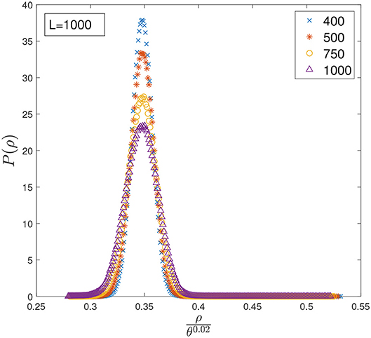
Figure 1. Distribution of densities P(ρ) computed at different values of θ and fixed L = 1, 000. The x-axis has been rescaled by θ^0.02 to align the peaks.

In Figures 2, 3 we plot the distribution of densities rescaling the x-axis by θ^ν, and tune ν to align the peaks of the distributions computed at different values of θ. Interestingly, in both cases the curves seem to collapse on the same shape for quite a wide range of θ, suggesting that the distribution has reached a stationary state and that increasing θ would imply only a shift of 〈ρ〉. However, increasing θ even further clearly shows that the asymptotic behavior suggested by the data collapse is only transient, as the curves start to deviate considerably from the shape observed at lower values of θ, as can be seen in Figure 4. Rescaling ρ by θ^0.005 one can align the position of the peaks in Figure 4 for θ ≳ 10⁴, but it is clear that, in order to perform a data collapse, the y-axis must be rescaled as well, as the height of the peaks decreases with θ.

FIGURE 2

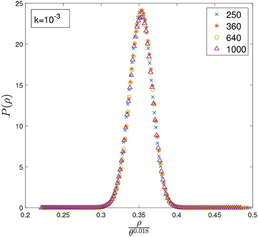
Figure 2. Distribution of densities P(ρ) computed at different values of θ and k = 10⁻³. Although rescaling the x-axis by θ^0.018 seems to make it possible to perform a data collapse for θ ∈ [250, 1000], this does not hold for larger values of θ.

FIGURE 3

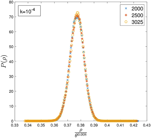
Figure 3. Distribution of densities P(ρ) computed at different values of θ and k = 10⁻⁴. Although rescaling the x-axis by θ^0.008 seems to make it possible to perform a data collapse for θ ∈ [2000, 3025], this does not hold for larger values of θ.

FIGURE 4

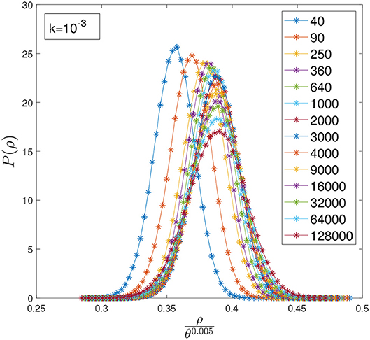
Figure 4. Distribution of densities P(ρ) computed at different values of θ and k = 10⁻³. The x-axis has been rescaled by θ^0.005 to align the position of the peaks at large values of θ.

For a fixed θ, we found that P(ρ) is well fitted by a Gaussian distribution. In Figure 5, we plot the mean and standard deviations of P(ρ) for k = 10⁻³ and find that the average density seemingly increases as a power-law for θ ≳ 10⁴, in agreement with the numerics presented in [5]. Although the mean μ(θ) seems to enter an asymptotic regime after θ ≳ 10⁴, it is less convincing whether the standard deviation σ(θ) has reached its asymptotic form.

FIGURE 5

Figure 5. Log-log plot of the mean and standard deviation of P(ρ) as a function of θ.

If we assume a Gaussian behavior for P(ρ) and that the mean and the standard deviation behave as

$\begin{array}{ll}\mu =a{\theta }^{{\nu }_{\mu }}\text{ and }\sigma =b{\theta }^{{\nu }_{\sigma }}.& (2)\end{array}$

then plotting P(ρ)σ(θ) vs. $\frac{\rho -\mu }{\sigma }$ should produce a standard normal distribution for systems at θ ≳ 10⁴. To estimate the asymptotic behavior, we used the last six data points for μ(θ) and the last three data points for σ(θ) in Figure 5, finding

$\begin{array}{l}a=0.388\pm 0.001\text{ and }{\nu }_{\mu }=0.0049\pm 0.0003\end{array}$

and

$\begin{array}{l}b=0.007\pm 0.004\text{ and }{\nu }_{\sigma }=0.099\pm 0.047\end{array}$

using 95% confidence bounds.

Using these estimates, we find that a data collapse seems to hold well for very large values of θ, as can be seen in Figure 6. However, such extrapolations have to be taken with great care, firstly because of the small data available for the fit and the not so convincing behavior of σ(θ), and secondly because the average density can never exceed 1, meaning that the apparent power-law growth has to stop at some point.

FIGURE 6

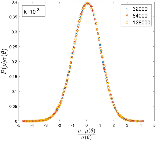
Figure 6. Data collapse for the distribution of densities P(ρ) and k = 10⁻³ obtained by inputting the estimated values of μ and σ into a Gaussian distribution. The x-axis and the y-axis have been rescaled in order to make all the curves collapse on a standard normal distribution.

Since ν_σ > ν_μ, the fluctuations grow at a faster rate than the average, as one would expect for a system close to criticality. From the ratio $\frac{\sigma (\theta )}{\mu (\theta )}~0.018·{\theta }^{0.094}$, one can obtain a crude estimate for when the fluctuations would become of the same order of magnitude as the average. This would happen at θ ~ 10¹⁸ and 〈ρ〉 ≃ 0.478. However, this argument can hardly hold, as it would imply that within two standard deviations, we would have values of the densities that exceed ρ = 1, which is, of course, impossible. Therefore, we can conclude that for k = 10⁻³ and within the Gaussian approximation, we can expect the standard deviation to be smaller than the average, despite growing at a faster rate.

As a reference, we computed a rough estimate of the value θ^* that would correspond to an average density equal to the percolation threshold $\mu ({\theta }^{*})={\rho }_p$. This gives θ^* ~ 10³⁷, which is consistent with the estimate made in [5] once the confidence bounds on a and ν_μ are taken into account for both datasets. However, there is no reason why the asymptotic density of the FFM should be the same as the critical percolation density, as even for very large systems the clusters would still be correlated and therefore intrinsically different from a percolation process.

Like previous studies of the FFM, we are unable to settle the true asymptotic scaling behavior of the model, which is still unreachable with today's computers. However, we showed that effectively, the distribution of densities remains Gaussian for very large system sizes and significant ranges of θ. In the next section, we will study the relationship between P(ρ) and the order parameters used in percolation and in [6], and show that P(ρ) defines a wide region where one can observe critical-like behavior.

3.2. The Most Frequently Visited Region

Even though the studies of precipitation [7] and brain activity [6] related their findings to critical behavior, both observed a remarkable broad onset of the order parameter, which is certainly not the behavior seen as one approaches the critical point of a second-order phase transition of an infinite system. The absence of a sharp onset of the order parameter is remarkable because, for system sizes like the earth atmosphere or the human brain, one would not expect any significant finite-size effect if the usual phenomenology of equilibrium phase transitions were any guidance.

While the activation dynamics characteristic of precipitation and brain phenomena are not at all similar to thermal equilibrium dynamics, both systems are at least at a schematic qualitative level similar to the dissipative dynamics of the FFM, with its cycles of loading and discharging. Here we want to investigate further the relationship between the distribution of residence times and the order parameter suggested in [10] and to determine to what extent the FFM exhibits an onset region similar to those observed in rain and brain. If that is the case, we may perhaps take this as indicative of a kind of "universality" different from the stringent universality definition we know from equilibrium systems and more of a pragmatic nature. Needless to say, could such a universality be established, it may be a great help in attempts to classify the behavior of activation dynamics in complex systems. Furthermore, it could be taken as indicative of a level of emergent behavior that is independent of the microscopic details, since rain and brain clearly do operate on totally different substrates.

We are of course just repeating the original hope of SOC research and suggesting that systems of entirely different nature may indeed exhibit similar emergent collective behavior, even if the dynamics does not operate in a critical state, but rather is found to inhabit a broad region of approximately scale-free nature. Crucial for our suggestion is the observation that the true asymptotic behavior of the FFM appears to happen for such enormous systems sizes that they hardly are of relevance to real macroscopic systems. In contrast, the quasi-scale free behavior observed in the FFM for intermediate system sizes [4, 5] may very well be helpful for the understanding of observations such as those presented in [6, 7].

To investigate the presence of a critical-like region in the FFM, we focus on the onset of measures that characterize the clusters of trees and keep track of the frequencies at which the system visits different regions of the parameter space. The order parameter for precipitation [7] was taken to be the precipitation rate and for the brain [6], the normalized size of the largest cluster of activated voxels in the fMRI scans—a choice that appears very natural in the light of ordinary percolation analysis.

In Figures 7, 8 we present the contour plot of the bivariate histograms of the average cluster size [11] 〈S〉 vs. the density ρ, and of the largest cluster normalized to the number of trees S_max vs. ρ. The color map represents the probability of observing a certain point in the parameter space, which is the same as the proportion of time spent by the system at that point. To create the heatmaps, we sampled 10⁷ configurations and grouped points with similar probabilities for better visual representation. Therefore, the histograms are not perfectly normalized. The study of both the average cluster size 〈S〉 and the normalized largest cluster S_max is inspired by the resemblance between the clusters of sites occupied by trees and the ordinary geometrical percolation transition. In percolation, either 〈S〉 or S_max are used to construct an order parameter.

FIGURE 7

Figure 7. Heatmap representing the bivariate histogram of the average cluster size and the density.

FIGURE 8

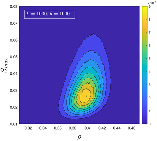
Figure 8. Heatmap representing the bivariate histogram of the normalized largest cluster and the density.

It is clear from the heat-maps that the density around ρ^* ≃ 0.4 stands out and that precisely like in the precipitation study [7], and even more so in the brain study [6], ρ^* is indicative of an onset of the order parameter. Furthermore, the region over which the creation of large events happens is very broad, and the system spends a significant fraction of time in the critical region. We know from the Gaussianity of P(ρ), see Figure 6, that this region stays broad for any reachable system size and values of θ. This very much suggests that the FFM's quasi-tuning to a critical region is a stylistic feature of important relevance.

3.3. The Distribution of the Largest Cluster

We now turn our attention to the non-normalized largest cluster, which we indicate with Λ to distinguish it from S_max. For a fixed system size and θ, we find that the distribution of the largest cluster P(Λ) is very well fitted by a Fréchet distribution, which corresponds to the class of extreme value statistics with a power-law tail. The good agreement of P(Λ) with a Fréchet distribution implies that the correlations between consecutive configurations generating the clusters are sufficiently weak to be ignored.

Although the distribution of cluster sizes does not obey simple scaling [4, 5], it was found in [12] that the distribution of instantaneous correlation lengths is scale-invariant for k = 10⁻³ and system sizes at least as big as θ = 9, 000. Given that P(λ) is fat-tailed, we now turn our attention to its scaling properties and see if simple scaling applies.

In order to measure Λ, one has to maintain and keep track of all clusters at all times, which makes the task more computationally intensive than just sampling the density ρ. For this reason, we analyzed systems sizes that are smaller than those used for the analysis of P(ρ). In our simulations, we used k = 10⁻³ and values of θ up to 4000, but we also checked the scaling for k = 5 · 10⁻⁴.

Assuming that simple scaling holds, we can expect P(Λ) to follow

$\begin{array}{ll}P(\Lambda )=aG\left(\frac{\Lambda }{{\Lambda }_c(\theta )}\right){\Lambda }^{-\tau }& (3)\end{array}$

for Λ₀ ≪ Λ ≪ Λ_c, where Λ₀ is a constant lower cutoff and Λ_c is an upper cutoff that diverges with θ. In Equation (3), a is a constant metric factor, τ is the critical exponent, and G is a universal function that decays quickly for Λ ≫ Λ_c. The form that is usually assumed for the upper cutoff is ${\Lambda }_c=b{\theta }^{\nu }$, where b is another constant metric factor and ν is the spatial dimensionality of the observable Λ [3].

If the data are consistent with the simple scaling ansatz, then it is possible to perform a data collapse by plotting P(Λ)Λ^τ vs. the rescaled variable $\frac{\Lambda }{{\Lambda }_c}$ for different values of θ. In Figure 9, we performed a data collapse using ν = 1.055 and τ = 1.04. We also estimated the critical exponents analyzing the first two moments of Equation (3) and fitting the data with $\langle \Lambda \rangle =c_1{\theta }^{{\alpha }_1}$ and $\langle {\Lambda }^2\rangle =c_2{\theta }^{{\alpha }_2}$, obtaining

$\begin{array}{l}{c}_1=10.7\pm 0.8\text{ and }{\alpha }_1=1.04\pm 0.01\end{array}$

and

$\begin{array}{l}{c}_2=110\pm 36\text{ and }{\alpha }_2=2.11\pm 0.04\end{array}$

using 95% confidence bounds.

FIGURE 9

Figure 9. Data collapse for the distribution of the largest cluster P(Λ) at k = 10⁻³.

From the exponents of the first two moments one can easily recover ν and τ using Equation (3):

$\begin{array}{ll}\nu ={\alpha }_2-{\alpha }_1\tau =2-\frac{{\alpha }_1}{\nu }& (4)\end{array}$

Using our estimates for α₁ and α₂, we get

$\begin{array}{ll}\nu =1.07\pm 0.04\tau =1.03\pm 0.04& (5)\end{array}$

using 95% confidence bounds.

These estimates for ν and τ are consistent with the ones obtained via data collapse and that have been used in Figure 9. Finally, we applied the whole procedure a second time using a smaller value of k, namely k = 5 · 10⁻⁴ and θ up to 2000. From the data collapse in Figure 10 we obtained an estimate of ν = 1.065 and τ = 1.04, while fitting the first two moments we obtained:

$\begin{array}{l}{c}_1=12.0\pm 0.7\text{ and }{\alpha }_1=1.05\pm 0.01\end{array}$

and

$\begin{array}{l}{c}_2=148\pm 15\text{ and }{\alpha }_2=2.12\pm 0.02\end{array}$

which are consistent with the data collapse and with those estimated for k = 10⁻³.

FIGURE 10

Figure 10. Data collapse for the distribution of the largest cluster P(Λ) at k = 5 · 10⁻⁴.

Although we had to restrict our simulations to values of θ < 10⁴, we observe a very robust scaling for the largest cluster Λ, which is not observed in the distribution of cluster sizes P(S) over the same range of θ [4]. Interestingly, we found that 〈Λ〉 ~ θ^1.04, a super-linear growth which indicates that the correlations in the system increase rapidly with θ. This behavior is consistent with the analysis of the distribution of instantaneous correlation lengths P(ξ) performed in [12], where it was found that the average instantaneous correlation length grows as 〈ξ〉 ~ θ^0.56 over the same range of θ.

4. Discussion

SOC was very much inspired by the successes of the renormalization group studies of equilibrium critical phenomena of the 1970-ties and its phenomenal understanding of the origin of universality classes. Initially, the discussions of SOC focused on accurately establishing the scaling behavior and related scaling exponents of the various models thought to represent the SOC phenomenology. The original sandpile model [1] was disappointingly far from simple scaling, and also the FFM turned out to behave very differently from the familiar scaling observed in equilibrium models such as the Ising model or geometrical percolation. Though there is at least one class of SOC models that exhibits clear scaling, namely the class represented by the Manna model [21], the beauty of strict scaling and universality classes defined by scaling exponents seems not to really capture the less than ideal critical behavior frequently observed in real systems, such as our two examples from rain and brain.

There is no doubt that the studies of the emergent dynamics of real complex systems from biology, geophysics, astrophysics, economics and more [22–24] keep identifying behavior which is qualitatively in the spirit of the hopes and dreams behind SOC, namely the lack of one characteristic scale in time and space, large fluctuations and no need for specific external tuning. So if the beauty of strict scaling and exact power laws does not carry over from equilibrium critical phenomena, the question is how we establish a systematic classification of the emergent phenomena observed in completely different systems. The study of the FFM and its comparison with the behavior of real systems suggests it is possible to establish a useful phenomenological understanding and classification reaching beyond the usual strict classification of universality classes defined in terms of shared scaling exponents.

The study presented here confirms earlier investigations of the behavior of the density ρ, and the change in the behavior of 〈ρ〉 for very large system sizes. Although we observed that the Gaussian behavior of P(ρ) holds at least until θ = 10⁵, we also showed that it is possible to obtain very good but deceitful data collapses for P(ρ) at different ranges of θ. If, on the one hand, this should serve as a warning for the analysis of the asymptotic scaling behavior of the FFM and other out of equilibrium systems, on the other hand, it shows that such effective scaling could be of guidance in the understanding and analysis of real systems that show similar dynamics.

Analyzing the average cluster size and the normalized largest cluster, we found that the FFM exhibits very similar behavior to the one observed in experimental studies of rain and brain [6, 7]. In particular, both studies and the FFM display a critical region over which both the residence time distribution and the order parameter peak up, meaning that the system spends most of the time in a highly susceptible state.

From the study of the largest cluster Λ it emerges that, although the FFM displays broken scaling in the distribution of cluster sizes, the distribution P(Λ) appears to be scale-invariant at least for θ < 10⁴. Furthermore, P(Λ) displays a super-linear growth of the first moment similar to the one observed for the average instantaneous correlation length in [12]. It is clear from the anomalous behavior of the density ρ that such results should be taken with care, as the model seems to enter a new regime when θ ≳ 10⁴. However, the robust scaling observed both in the largest cluster and in the instantaneous correlation length suggests that at least for system sizes below θ = 10⁴ there is a fast and scale-free growth of the correlations with the activity θ.

Although the FFM does not display the reassuring scaling observed in equilibrium models, its phenomenology appears to summarize elegantly and robustly the emergent dynamics of spreading and recharging seen in such disparate phenomena as rain precipitation and brain dynamics. Moreover, examples of broken scaling and non-exact powerlaws are ubiquitous in nature and in the scientific literature [25] and, for this reason, we believe that the characteristic behavior of the FFM should be seen as an asset rather than a limitation of the model.

Data Availability Statement

The original contributions presented in the study are included in the article/Supplementary Material, further inquiries can be directed to the corresponding author.

Author Contributions

LP performed the numerical simulations and analyses and produced the figures. Both authors discussed the results of the simulations and jointly wrote the manuscript.

Funding

LP gratefully acknowledges an EPSRC-Roth scholarship (Award Reference No. 1832407) from EPSRC and the Department of Mathematics at Imperial College London.

Conflict of Interest

The authors declare that the research was conducted in the absence of any commercial or financial relationships that could be construed as a potential conflict of interest.

Acknowledgments

LP thankfully acknowledges the High-Performance Computing facilities provided by the Imperial College Research Computing Service (DOI: 10.14469/hpc/2232).

Supplementary Material

The Supplementary Material for this article can be found online at: https://www.frontiersin.org/articles/10.3389/fphy.2020.00257/full#supplementary-material

References

1. Bak P, Tang C, Wiesenfeld K. Self-organized criticality: an explanation of the 1/f noise. Phys Rev Lett. (1987) 59:381–4. doi: 10.1103/PhysRevLett.59.381

PubMed Abstract | CrossRef Full Text | Google Scholar

2. Drossel B, Schwabl F. Self-organized critical forest-fire model. Phys Rev Lett. (1992) 69:1629–32. doi: 10.1103/PhysRevLett.69.1629

PubMed Abstract | CrossRef Full Text | Google Scholar

3. Pruessner G. Self-Organised Criticality: Theory, Models and Characterisation. Cambridge: Cambridge University Press (2012).

Google Scholar

4. Pruessner G, Jensen HJ. Broken scaling in the forest-fire model. Phys Rev E. (2002) 65:056707. doi: 10.1103/PhysRevE.65.056707

PubMed Abstract | CrossRef Full Text | Google Scholar

5. Grassberger P. Critical behaviour of the Drossel-Schwabl forest fire model. N J Phys. (2002) 4:17. doi: 10.1088/1367-2630/4/1/317

CrossRef Full Text | Google Scholar

6. Tagliazucchi E, Balenzuela P, Fraiman D, Chialvo D. Criticality in large-scale brain fMRI dynamics unveiled by a novel point process analysis. Front Physiol. (2012) 3:15. doi: 10.3389/fphys.2012.00015

PubMed Abstract | CrossRef Full Text | Google Scholar

7. Peters O, Neelin JD. Critical phenomena in atmospheric precipitation. Nat Phys. (2006) 2:393–6. doi: 10.1038/nphys314

CrossRef Full Text | Google Scholar

8. Sornette D. Critical phase transitions made self-organized : a dynamical system feedback mechanism for self-organized criticality. J Phys I France. (1992) 2:2065–73.

Google Scholar

9. Zapperi S, Lauritsen KB, Stanley HE. Self-organized branching processes: mean-field theory for avalanches. Phys Rev Lett. (1995) 75:4071–4. doi: 10.1103/PhysRevLett.75.4071

PubMed Abstract | CrossRef Full Text | Google Scholar

10. Palmieri L, Jensen HJ. The emergence of weak criticality in SOC systems. Europhys Lett. (2018) 123:20002. doi: 10.1209/0295-5075/123/20002

CrossRef Full Text | Google Scholar

11. Christensen K, Moloney NR. Complexity and Criticality. London: Imperial College Press (2005).

PubMed Abstract | Google Scholar

12. Palmieri L, Jensen HJ. Investigating critical systems via the distribution of correlation lengths. Phys Rev Res. (2020) 2:013199. doi: 10.1103/PhysRevResearch.2.013199

CrossRef Full Text | Google Scholar

13. Bak P, Chen K, Tang C. A forest-fire model and some thoughts on turbulence. Phys Lett A. (1990) 147:297–300. doi: 10.1016/0375-9601(90)90451-S

CrossRef Full Text | Google Scholar

14. Henley CL. Self-organized percolation: a simpler model. Bull Am Phys Soc. (1989) 34:838.

Google Scholar

15. Grassberger P. On a self-organized critical forest-fire model. J Phys A Math Gen. (1993) 26:2081–9. doi: 10.1088/0305-4470/26/9/007

CrossRef Full Text | Google Scholar

16. Clar S, Drossel B, Schwabl F. Scaling laws and simulation results for the self-organized critical forest-fire model. Phys Rev E. (1994) 50:1009–18. doi: 10.1103/PhysRevE.50.1009

PubMed Abstract | CrossRef Full Text | Google Scholar

17. Schenk K, Drossel B, Clar S, Schwabl F. Finite-size effects in the self-organized critical forest-fire model. Eur Phys J B Condens Matter Complex Syst. (2000) 15:177–85. doi: 10.1007/s100510051113

CrossRef Full Text | Google Scholar

18. Pruessner G, Jensen HJ. Efficient algorithm for the forest fire model. Phys Rev E. (2004) 70:066707. doi: 10.1103/PhysRevE.70.066707

PubMed Abstract | CrossRef Full Text | Google Scholar

19. Honecker A, Peschel I. Length scales and power laws in the two-dimensional forest-fire model. Phys A Stat Mech Appl. (1997) 239:509–30.

Google Scholar

20. Pastor-Satorras R, Vespignani A. Corrections to scaling in the forest-fire model. Phys Rev E. (2000) 61:4854–9. doi: 10.1103/PhysRevE.61.4854

PubMed Abstract | CrossRef Full Text | Google Scholar

21. Manna SS. Two-state model of self-organized criticality. J Phys A Math Gen. (1991) 24:L363–9. doi: 10.1088/0305-4470/24/7/009

CrossRef Full Text | Google Scholar

22. Ball P. Critical Mass. How One Thing Leads to Another. New York, NY: Farrar, Straus and Giroux (2004).

23. West G. Scale: The Universal Laws of Life and Death in Organisms, Cities and Companies. London: The Orion Publishing Group (2018).

24. Krakauer DC editor. Worlds Hidden in Plain Sight. Santa Fe, NM: The Santa Fe Institute Press (2019).

25. Clauset A, Shalizi CR, Newman MEJ. Power-law distributions in empirical data. SIAM Rev. (2009) 51:661–703. doi: 10.1137/070710111

CrossRef Full Text | Google Scholar