The Capon Method for Mercury's Magnetic Field Analysis

Characterization of Mercury's internal and external magnetic field is one of the primary goals of the magnetometer experiment on board the BepiColombo MPO (Mercury Planetary Orbiter) spacecraft. A novel data analysis tool is developed to determine the Gauss coefficients in the multipole expansion using Capon's minimum variance projection method. The construction of the estimator is presented along with a test against the numerical simulation data of Mercury's magnetosphere and a comparison with the least square fitting method shows, that Capon's estimator is in better agreement with the coefficients, implemented in the simulation, than the least square fit estimator.

1. Introduction

The reconstruction of planetary magnetic fields is one of the most important goals of a magnetometer experiment on board an orbiting spacecraft. Various inversion methods have successfully been applied to the data of former missions that visited different planets in our solar system. For example, generalized inversion [1] and elastic net regression [2] have been applied to the reconstruction of Jupiter's internal magnetic field. The weighted least square fit [3] and robust regression [4] appeared as useful methods for the analysis of Saturn's magnetic field. The Earth's magnetic field has been analyzed among other methods by using the maximum entropy method [5]. All these methods will be useful tools for Mercury's magnetic field analysis, which is one of the primary goals of the magnetometer experiment on board the BepiColombo mission. In this work we present an alternative method, namely Capon's method, for the analysis of Mercury's internal magnetic field.

Capon's method [6], also known as minimum variance distortionless response estimator (MVDR) [7], was introduced for reconstructing the velocities and wave vectors of seismic waves measured on an array of sensors on the Earth's surface. In space plasma physics, the method has first been successfully applied to the analysis of plasma waves in the terrestrial magnetosphere [8]. Later on, the method was extended for the mode decomposition of magnetic fields [9]. This establishes a basis to separate the planetary magnetic field from the total measured field in Mercury's magnetosphere.

The separation of the internal magnetic field from the external parts of the field, which are generated by currents flowing in the magnetosphere is important for the reconstruction of the internal field. There exists a paraboloid model of Mercury's magnetosphere [10] which has successfully been applied to the analysis of Mercury's internal magnetic field [11, 12]. Since Capon's method is applied to the analysis of Mercury's internal magnetic field for the first time, here only the internal parts of the field are considered in the parametrization as a proof of concept.

Concerning to the BepiColombo mission, in this work magnetic field data resulting from the plasma interaction of Mercury with the solar wind are simulated and Capon's method is applied to the magnetic field data to analyze Mercury's internal magnetic field.

2. Parametrization and Inversion Methods

2.1. Parametrization of Mercury's Magnetic Field

The parametrization of planetary magnetic fields is based on the Gauss representation [13]. If only data in curl-free regions are analyzed, Ampère's law ∂_x × B = 0, where B is the magnetic field vector and ∂_x is the spatial derivative, yields the existence of a scalar potential Φ, so that B = −∂_xΦ. In general, Φ is composed of internal and external parts. In the following only the internal parts Φ_i will be considered. For the parametrization of the internal dipole and quadrupole fields the scalar potential is expanded into spherical harmonics

$\begin{array}{l}{\Phi }_i=R_M{{\displaystyle \sum _{l=1}^2\left(\frac{R_M}{r}\right)}}^{l+1}{\displaystyle \sum _{m=0}^l[g_l^m\cos (m\lambda )}\\ +h_l^m\sin (m\lambda )]P_l^m\left(\cos (\theta )\right)& (1)\end{array}$

where planetary centered coordinates with radius r, azimuth angle λ∈[0, 2π], and polar angle θ∈[0, π] are chosen. R_M indicates the radius of Mercury and $P_l^m$ are the Schmidt-normalized associated Legendre polynomials of degree l and order m. The expansion coefficients $g_l^m$ and $h_l^m$ are the internal Gauss coefficients. Arranging the Gauss coefficients into a vector $\underset{\_}{g}:={\left(g_1^0,g_1^1,h_1^1,g_2^0,g_2^1,h_2^1,g_2^2,h_2^2\right)}^T$, for later application called ideal coefficient vector, the contribution of the internal magnetic field can be rearranged as

$\begin{array}{ll}\underset{\_}{B}=-{\partial }_{\underset{\_}{x}}{\Phi }_i=\underset{\_}{\underset{\_}{H}}\underset{\_}{g},& (2)\end{array}$

where the terms of the multipole series are arranged in the matrix $\underset{\_}{\underset{\_}{H}}$(r,θ,λ). The magnetic field measurements B and the underlying model $\underset{\_}{\underset{\_}{H}}$ are known. The unknown coefficient vector g is to be determined. In most applications the number of known magnetic data points is much larger than the number of the expansion coefficients, resulting in an overdetermined inversion problem. Therefore, $\underset{\_}{\underset{\_}{H}}$ is a rectangular matrix in general and the direct inversion of Equation (2) is impossible. But there exist several inversion methods for estimating g [7].

2.2. Least Square Fit (LSF) Method

The most commonly used method for inverse problems is the least square fit method. The method minimizes the quadratic deviation between the disturbed measurements B and the model $\underset{\_}{\underset{\_}{H}}$ [7]

$\begin{array}{ll}\underset{\underset{\_}{g}}{\text{min}}{\left|\underset{\_}{\underset{\_}{H}}\underset{\_}{g}-\underset{\_}{B}\right|}^2=\underset{g_l}{\text{min}}\left(g_i{H}_{ij}^{†}{H}_{jk}{g}_k-2B_j{H}_{ji}{g}_i+B_i{B}_i\right),& (3)\end{array}$

Providing us

$\begin{array}{ll}{\partial }_{g_l}{\left|\underset{\_}{\underset{\_}{H}}\underset{\_}{g}-\underset{\_}{B}\right|}^2=0,& (4)\end{array}$

where † symbolizes the Hermitian adjunction. The LSF estimator g_L realizing the minimal deviation is given by

$\begin{array}{ll}{\underset{\_}{g}}_L={\left[{\underset{\_}{\underset{\_}{H}}}^{†}\underset{\_}{\underset{\_}{H}}\right]}^{-1}{\underset{\_}{\underset{\_}{H}}}^{†}\underset{\_}{B}.& (5)\end{array}$

2.3. Capon's Method

Capon's method is based on the construction of a filter matrix $\underset{\_}{\underset{\_}{w}}$ so that the output power

$\begin{array}{ll}\text{tr}\left[{\underset{\_}{\underset{\_}{w}}}^{†}\underset{\_}{\underset{\_}{M}}\underset{\_}{\underset{\_}{w}}\right]& (6)\end{array}$

is minimized with respect to $\underset{\_}{\underset{\_}{w}}$, subject to the distortionless constraint

$\begin{array}{ll}{\underset{\_}{\underset{\_}{w}}}^{†}\underset{\_}{\underset{\_}{H}}=\underset{\_}{\underset{\_}{I}},& (7)\end{array}$

where $\text{tr}\left[{\underset{\_}{\underset{\_}{w}}}^{†}\underset{\_}{\underset{\_}{M}}\underset{\_}{\underset{\_}{w}}\right]$ is the trace of the matrix ${\underset{\_}{\underset{\_}{w}}}^{†}\underset{\_}{\underset{\_}{M}}\underset{\_}{\underset{\_}{w}}$ and $\underset{\_}{\underset{\_}{I}}$ is the identity matrix. The matrix $\underset{\_}{\underset{\_}{M}}:=\langle \underset{\_}{B}°\underset{\_}{B}\rangle$ is called the data covariance matrix, where the angular brackets indicate averaging over ensemble, e.g., different samples, realizations, or measurements. The error of the magnetic data is assumed to be Gaussian with variance σ_n and zero mean. In this case, the data covariance matrix can be written as $\underset{\_}{\underset{\_}{M}}=\langle \underset{\_}{B}\rangle °\langle \underset{\_}{B}\rangle +{\sigma }_n^2\underset{\_}{\underset{\_}{I}}$. Capon's estimator realizing the minimal output power, subject to the distortionless constraint, results in [9]

$\begin{array}{ll}{\underset{\_}{g}}_C={\left[{\underset{\_}{\underset{\_}{H}}}^{†}{\underset{\_}{\underset{\_}{M}}}^{-1}\underset{\_}{\underset{\_}{H}}\right]}^{-1}{\underset{\_}{\underset{\_}{H}}}^{†}{\underset{\_}{\underset{\_}{M}}}^{-1}\langle \underset{\_}{B}\rangle ,& (8)\end{array}$

which has the same structure as the LSF estimator (Equation 4), but with additional weighting by the covariance matrix. This demonstrates that the Capon filter discriminates between preferred and deprived data whereas the LSF treats all data equally. Adding a constant value ${\sigma }_d^2$ to the diagonal of the covariance matrix improves the robustness of Capon's estimator [14]. The diagonal loaded covariance matrix results in

$\begin{array}{ll}\underset{\_}{\underset{\_}{M}}=\langle \underset{\_}{B}\rangle °\langle \underset{\_}{B}\rangle +{\sigma }^2\underset{\_}{\underset{\_}{I}},& (9)\end{array}$

where ${\sigma }^2:={\sigma }_n^2+{\sigma }_d^2$.

3. Simulation of Mercury's Magnetic Field

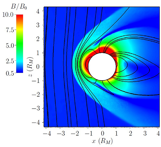
For the evaluation of Capon's estimator in comparison with the LSF estimator simulated magnetic field data are analyzed. The data are simulated with the hybrid code AIKEF [15], that has successfully been applied to several problems in Mercury's plasma interaction [16]. The internal Gauss coefficients $g_1^0=-190\mathrm{\text{nT}}$ and $g_2^0=-78\mathrm{\text{nT}}$ [17], defining the non-vanishing components of the ideal coefficient vector g (Equation 2), are implemented in the simulation code and the magnetic field resulting from the interaction of Mercury with the solar wind is simulated. The solar wind velocity of 400km/s is orientated parallel to the x-axis and the solar wind magnetic field with B₀ = 20nT is orientated toward the z-axis. The y-axis completes the right hand system. The solar wind density was chosen to 30cm⁻³. In Figure 1, the simulated magnitude of the magnetic field B is displayed in the x-z-plane (meridional plane).

FIGURE 1

Figure 1. Simulated magnitude of the magnetic field B in multiples of the solar wind magnetic field B₀ = 20nT in the x-z-plane. The black lines describe the magnetic field lines. The white circle of radius 1R_M symbolizes Mercury. The implemented internal Gauss coefficients are $g_1^0=-190\mathrm{\text{nT}}$ and $g_2^0=-78\mathrm{\text{nT}}$ [17].

4. Application and Discussion

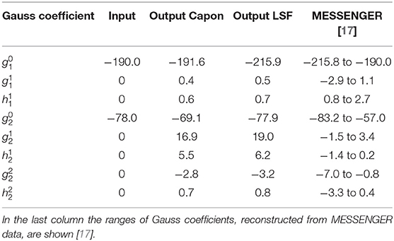
Now Capon's method is applied to the simulated data for reconstructing the ideal Gauss coefficients implemented in the simulation. The comparison of Capon's estimator g_C with the ideal coefficient vector g enables the judgement of the method. To classify the role of Capon's method in terms of the diversity of existing inversion methods, Capon's estimator furthermore is compared with the LSF estimator g_L. The data are evaluated at an ensemble of data points with distance 0.2R_M from the surface on the night side of Mercury (x < 0). The reconstructed Gauss coefficients are presented in Table 1.

TABLE 1

Table 1. Capon's and LSF estimators for the internal Gauss coefficients in nT.

The underlying model only describes the internal magnetic field $\underset{\_}{\underset{\_}{H}}\underset{\_}{g}$. The external parts of the field $b:=\underset{\_}{B}-\underset{\_}{\underset{\_}{H}}\underset{\_}{g}$ are not parameterized. Thus, the deviation of the LSF estimator and the ideal coefficient vector is given by

$\begin{array}{ll}|{\underset{\_}{g}}_L-\underset{\_}{g}|=\left|{\left[{\underset{\_}{\underset{\_}{H}}}^{†}\underset{\_}{\underset{\_}{H}}\right]}^{-1}{\underset{\_}{\underset{\_}{H}}}^{†}\underset{\_}{b}\right|\approx 32.9\text{nT},& (10)\end{array}$

whereas the difference between Capon's estimator and the ideal coefficient vector results in

$\begin{array}{ll}|{\underset{\_}{g}}_C-\underset{\_}{g}|=|{\left[{\underset{\_}{\underset{\_}{H}}}^{†}{\underset{\_}{\underset{\_}{M}}}^{-1}\underset{\_}{\underset{\_}{H}}\right]}^{-1}{\underset{\_}{\underset{\_}{H}}}^{†}{\underset{\_}{\underset{\_}{M}}}^{-1}\underset{\_}{b}|\approx 20.1\text{nT}.& (11)\end{array}$

To judge the quality of Capon's estimator the comparison of individual coefficients presented in Table 1 is not a vital metric. For example, the Gauss coefficient $g_2^0$ reconstructed by the LSF method is in better agreement with the ideal coefficient than the coefficient estimated by Capon's method. But for all coefficients together g_C−g<g_L−g holds.

Therefore, Capon's estimator is in better agreement with the ideal coefficient vector than the LSF estimator.

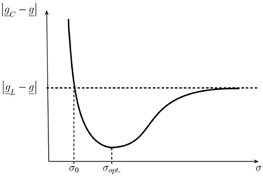
The choice of the diagonal loading parameter ${\sigma }_d^2$ is essential for the difference g_C−g. The diagonal loaded covariance matrix results from the additional quadratic constraint $\text{tr}\left({\underset{\_}{\underset{\_}{w}}}^{†}\underset{\_}{\underset{\_}{w}}\right)=T_0$, where T₀ = const. and ${\sigma }_d^2$ is the corresponding Lagrange multiplier [14]. The choice of T₀ controls the diagonal loading parameter ${\sigma }_d^2$ and defines how the data will be weighted by the filter matrix $\underset{\_}{\underset{\_}{w}}$. It depends on the underlying model and the evaluated data. Figure 2 illustrates how σ in principle controls the difference g_C−g. For σ → 0 Capon's estimator shows a large deviation to g. If σ → ∞, Capon's estimator approaches the LSF estimator. But if the data are not completely described by the model (b≠0) there exists a parameter $\sigma =\sqrt{{\sigma }_n^2+{\sigma }_d^2}={\sigma }_0$, so that for all σ≥σ₀

$\begin{array}{ll}|{\underset{\_}{g}}_C-\underset{\_}{g}|\le |{\underset{\_}{g}}_L-\underset{\_}{g}|.& (12)\end{array}$

Furthermore it even exists an optimal parameter σ_opt., that realizes the best agreement between Capon's estimator and g. For the results presented in Table 1 this optimal parameter is σ_opt.≈276nT.

FIGURE 2

Figure 2. Sketch of the deviation g_C−g between Capon's estimator g_C and the ideal coefficient vector g subject to σ. For large σ → ∞ the deviation converges to the deviation of the least-square-fit estimator g_L and the implemented coefficient vector g. There exists σ₀ so that g_C−g ≤g_L−g, for all σ≥σ₀, and an optimal parameter σ_opt., that realizes the best agreement between Capon's estimator an the ideal coefficient vector.

Since the choice of σ controls $\text{tr}\left({\underset{\_}{\underset{\_}{w}}}^{†}\underset{\_}{\underset{\_}{w}}\right)$, the value of the optimal diagonal loading parameter is not directly related with an error of the magnetic measurements. More likely σ_opt. can be understood as a parameter that measures the model mismatches.

When Capon's method is applied to real spacecraft data, the ideal coefficient vector g is not available anymore and therefore the deviation g_C−g cannot be used as metric for calculating the optimal diagonal loading parameter. In this case, there exist other methods for estimating σ_opt., e.g. the L-curve method, that solely depend on the underlying model and the data [18].

5. Summary and Outlook

In this work Capon's method has been applied to simulated magnetic field data to analyze Mercury's internal magnetic field. The internal field, parameterized by the internal Gauss coefficients, was implemented in the simulation code AIKEF and the magnetic field resulting from the plasma interaction of Mercury and the solar wind was simulated. The comparison of Capon's method and the commonly used least square fit method showed that Capon's estimator is in better agreement with the implemented Gauss coefficients than the least square fit estimator. A helpful procedure is the diagonal loading of the data covariance matrix, that improves the robustness of Capon's estimator. It turns out that there exists an optimal diagonal loading parameter where Capon's estimator is nearest to the ideal coefficient vector.

Since only the internal magnetic field was parameterized, Capon's estimator shows some deviation to the implemented coefficients. Additional parameterizing of the external contributions of the magnetic field, for example by using the paraboloid model for Mercury's magnetosphere [10], may still improve Capon's estimator, especially when data points are collected in some distance above the planetary surface. Moreover, this enables us to reconstruct higher-order terms such as octupole terms. Furthermore, as the Gauss representation is restricted to curl-free regions, the Mie representation (poloidal-toroidal decomposition) would extend the data collection to regions where electrical currents flow.

Data Availability Statement

The raw data supporting the conclusions of this article will be made available by the authors, without undue reservation.

Author Contributions

All authors contributed conception and design of the study. DH organized the database. ST, YN, and UM performed the statistical analysis and wrote the first draft of the manuscript. All authors contributed to manuscript revision, read, and approved the submitted version.

Funding

We acknowledge support by the German Research Foundation and the Open Access Publication Funds of the Technische Universität Braunschweig. This work by YN was supported by the Austrian Space Applications Programme at the Austrian Research Promotion Agency under contract 865967. DH was supported by the German Ministerium für Wirtschaft und Energie and the German Zentrum für Luft- und Raumfahrt under contract 50 QW1501.

Conflict of Interest

The authors declare that the research was conducted in the absence of any commercial or financial relationships that could be construed as a potential conflict of interest.

Acknowledgments

The authors are grateful for stimulating discussions and helpful suggestions by Karl-Heinz Glassmeier, Patrick Kolhey, and Alexander Schwenke.

References

1. Connerney JEP. The magnetic field of Jupiter: a generalized inverse approach. J Geophys Res. (1981) 86:7679–93. doi: 10.1029/JA086iA09p07679

CrossRef Full Text | Google Scholar

2. Moore KM, Bloxham J, Connerney JEP, Jørgensen JL, Merayo JMG. The analysis of initial Juno magnetometer data using a sparse magnetic field representation. Geophys Res Lett. (2017) 44:4687–93. doi: 10.1002/2017GL073133

CrossRef Full Text | Google Scholar

3. Davis L, Smith EJ. New models of Saturn's magnetic field using Pioneer 11 vector helium magnetometer data. J Geophys Res. (1986) 91:1373–80. doi: 10.1029/JA091iA02p01373

CrossRef Full Text | Google Scholar

4. Cao H, Russell CT, Christensen UR, Dougherty MK, Burton ME. Saturn's very axisymmetric magnetic field: no detectable secular variation or tilt. Earth Planet Sci. (2011) 304:22–8. doi: 10.1016/j.epsl.2011.02.035

CrossRef Full Text | Google Scholar

5. Jackson A. Intense equatorial flux spots on the surface of the Earth's core. Nature. (2003) 424:760–3. doi: 10.1038/nature01879

PubMed Abstract | CrossRef Full Text | Google Scholar

6. Capon J. High resolution frequency-wavenumber spectrum analysis. Proc IEEE. (1969) 57:1408–18. doi: 10.1109/PROC.1969.7278

CrossRef Full Text | Google Scholar

7. Haykin S. Adaptive Filter Theory. 2nd Edn. Prentice Hall Information and System Science Series. New Jersey: Prentice-Hall Inc. (1991).

Google Scholar

8. Motschmann U, Woodward TI, Glassmeier KH, Southwood DJ, Pinçon JL. Wavelength and direction filtering by magnetic measurements at satellite arrays: generalized minimum variance analysis. J Geophys Res. (1996) 101:4961–6. doi: 10.1029/95JA03471

CrossRef Full Text | Google Scholar

9. Narita Y. A note on Capon's minimum variance projection for multi-spacecraft data analysis, Front Phys. (2019) 7:8. doi: 10.3398/fphy.2019.00008

CrossRef Full Text | Google Scholar

10. Alexeev II, Belenkaya ES, Bobrovnikov S, Slavin Yu, Sarantos JA. Paraboloid model of Mercury's magnetosphere. JGR. (2008) 113: doi: 10.1029/2008JA013368

CrossRef Full Text | Google Scholar

11. Alexeev II, Belenkaya ES, Slavin JA, Korth H, Anderson BJ, Baker DN, et al. Mercury's magnetospheric magnetic field after the first two MESSENGER flybys. Icarus. (2010) 209:23–39. doi: 10.1016/j.icarus.2010.01.024

CrossRef Full Text | Google Scholar

12. Johnson CL, Purucker ME, Korth H, Anderson BJ, Winslow RM, Al Asad MMH, et al. MESSENGER observations of Mercury's magnetic field structure. JGR. (2012) 117:E00L14. doi: 10.1029/2012JE004217

CrossRef Full Text | Google Scholar

13. Gauß CF. Allgemeine Theorie des Erdmagnetismus: Resultate aus den Beobachtungen des Magnetischen Vereins im Jahre 1838. (1839).

Google Scholar

14. Van Trees HL. Detection, Estimation, and Modulation Theory, Optimum Array Processing. New York, NY: Wiley (2002).

Google Scholar

15. Mueller J, Simon S, Motschmann U, Schuele J, Glassmeier K-H, Pringle GJ. A.I.K.E.F.: adaptive hybrid model for space plasma simulations. Comput Phys Commun. (2011) 182:946–66. doi: 10.1016/j.cpc.2010.12.033

CrossRef Full Text | Google Scholar

16. Exner W, Heyner D, Liuzzo L, Motschmann U, Shiota D, Kusano K, et al. Coronal mass ejection hits mercury: AIKEF hybrid-code results compared to MESSENGER data. Planet Space Sci. (2018) 153:89–99. doi: 10.1016/j.pss.2017.12.016

CrossRef Full Text | Google Scholar

17. Wardinski I, Langlais B, Thébault E. Correlated time-varying magnetic field and the core size of mercury. J Geophys Res. (2019) 124:2178–97. doi: 10.1029/2018JE005835

CrossRef Full Text | Google Scholar

18. Hiemstra JH, Wippert MW, Goldstein JS, Pratt T. Application of the L-curve technique to loading level determination in adaptive beamforming. In: Conference Record of the Thirty-Sixth Asilomar Conference on Signals, Systems and Computers. Pacific Grove, CA (2002).

Google Scholar