
95% of researchers rate our articles as excellent or good
Learn more about the work of our research integrity team to safeguard the quality of each article we publish.
Find out more
BRIEF RESEARCH REPORT article
Front. Phys. , 28 July 2020
Sec. Statistical and Computational Physics
Volume 8 - 2020 | https://doi.org/10.3389/fphy.2020.00211
This article is part of the Research Topic Mathematical Treatment of Nanomaterials and Neural Networks View all 28 articles
 Hassan Raza
 Ying Ji*
Let Γ = (V, E) be a connected graph. A vertex i ∈ V recognizes two elements (vertices or edges) j, k ∈ E ∩ V, if dΓ(i, j) ≠ dΓ(i, k). A set S of vertices in a connected graph Γ is a mixed metric generator for Γ if every two distinct elements (vertices or edges) of Γ are recognized by some vertex of S. The smallest cardinality of a mixed metric generator for Γ is called the mixed metric dimension and is denoted by βm. In this paper, the mixed metric dimension of a generalized Petersen graph P(n, 2) is calculated. We established that a generalized Petersen graph P(n, 2) has a mixed metric dimension equivalent to 4 for n ≡ 0, 2(mod4), and, for n ≡ 1, 3(mod4), the mixed metric dimension is 5. We thus determine that each graph of the family of a generalized Petersen graph P(n, 2) has a constant mixed metric dimension.
2010 Mathematics Subject Classification: 05C12, 05C90
The aim of robot navigation functionality is to attain the coveted position promptly whenever it is desired. Let us imagine that robot navigation in a sensor network that can obtain the distances to a collection of landmarks. A robot's position is solely resolved by determining the subset of nodes in the sensor network. It can be achieved by the concept of landmarks in the graphs introduced in Khuller et al. [1]; this idea was later named the metric dimension. All the graphs considered here have no loops and are simple, measurable, and undirected.
Let Γ = (V, E) be the graph of the distance dΓ(a, b) (or d(a, b)) among the vertices a, b ∈ V(Γ) the minimum length of paths between them. For a vertex a ∈ V, distinguish two vertices in a graph, say b and c, if the condition dΓ(a, b) ≠ dΓ(a, c) holds. A set R ⊂ V(Γ) is the metric generator if some chosen vertices of the set R recognizes a pair of distinguished vertices. The metric basis with the least number of elements is called the metric generator, and the cardinality of its metric basis is termed the metric dimension. The notation employed here is β(Γ). The fundamental concept of the metric dimension was instated by Slater [2], and the notation of the metric dimension was initiated by Haray and Melter [3]. This concept was later studied by many researchers with unique modifications; for reference, see [4–8]. Some of the recent results on metric dimension and its further variations are studied in Shao et al. [9] and Raza et al. [10–13].
Lemma 1. Suppose R is the distinguishing set of Γ and the vertices a, b ∈ V(Γ). If dΓ(a, c) ≠ dΓ(a, c), for all vertices c ∈ V(Γ)\{a, b}, then {a, b}⋂R ≠ ∅.
Analogous to this definition, Kelenc et al. [14] introduced the concept of edge metric dimension, and this was further studied in Zubrilina [15], Peterin and Yero [16], and Zhu et al. [17]. This distance between an edge e = ab and a vertex c is given as follows
A vertex c ∈ V(Γ) distinguishes two edges of a graph e1, e2 ∈ E(Γ) if dΓ(e1, u) ≠ dΓ(e2, u). The set Re ⊂ V is termed as the edge metric generator if some distinct edges of Γ are distinguished by the vertex set Re. The cardinality of an edge metric generator is called an edge metric dimension, and it is depicted as βe(Γ). Having defined the notion of an edge metric generator, which distinctly recognizes every edge in a graph, a common assumption would be that any edge metric generator Re would be a metric dimension as well. This assumption is far from reality, as indicated in Kelenc et al. [14], but there are several families of graphs where this occurs, that is, β(Γ) = βe(Γ). Some other distance related parameters are studied in Liu et al. [18–22].
In this paper, our focus is on mixed metric dimension, which is a mixed version of metric and edge metric dimension. A set Rm of vertices of a graph Γ is known as a mixed metric generator if any two distinct elements (vertices or edges) of a graph are recognized by some the vertex set of Rm. The least cardinality of a mixed metric generator for a graph is termed as a mixed metric dimension, denoted as βm(Γ). The idea is recently brought forward by Kelenc et al. [23].
Lemma 2. Let for some vertex a ∈ V(Γ), and let Rm = V(Γ)\a, and if there is an element b ∈ N(a), also for some c ∈ Rm, dΓ(ab, c) ≠ dΓ(b, c), then Rm is the mixed metric generator for the graph Γ.
The notion of a mixed metric dimension clearly indicates that a mixed metric generator is also a standard metric generator and an edge metric generator, The following relationship is given in [23],
The following remark shows the structure of mixed metric dimension:
Remark 1: [23] Suppose for some graph Γ we have 2 ≤ βm ≤ n. Recently, this concept has attracted some attention, and it has been studied by Raza et al. [24]. The authors discussed the mixed metric dimension among the prism graphs, which are commonly known as generalizes Petersen graphs P(n, 1), and two families of convex polytopes An, Rn, further presenting the problem of finding βm(P(n, 2)).
Some of the results regarding metric and edge metric dimension are given:
Remark 2: [14] For n ≥ 2, the metric and edge metric dimension are, ; for cycle graph, ; for complete graph, ; and for any complete bipartite graph different from , .
Next, we present some already known results for βm,
Proposition 1: [23] For a path graph order n ≥ 4, we have .
Proposition 2: [23] Let us consider any two positive integers: e, f
Proposition 3: [23] For a grid graphs, Pm□Pn, with m ≥ n ≥ 2, βm = 3.
Proposition 4: [23] Let us assume cycle graph of order n ≥ 4, then βm(Cn) = 3.
Lemma 3. [24]The mixed metric generator Rm must contain vertices from both the outer and inner cycle for the prism graph Dn.
Proof: For P(n, 1), this holds, and, by the same intuition, this must be true for P(n, 2). The mixed metric resolving set comprises of vertices from both the cycles, which contain vertices of outer and inner cycle, respectively. □
The generalized Petersen graphs is introduced by Watkins [25]. The P(n, ℓ), where n ≥ 3 and (see Figure 2), which is the cubic graph consists of vertices and edges, is shown below.
Example: We used the graph of P(n, 8), as can be seen in Figure 1. The mixed metric generator for P(n, 8) is βm = {q0, q1, p4, p5}, and it can been seen from Table 1 that all the representation of vertices and edges are distinct.
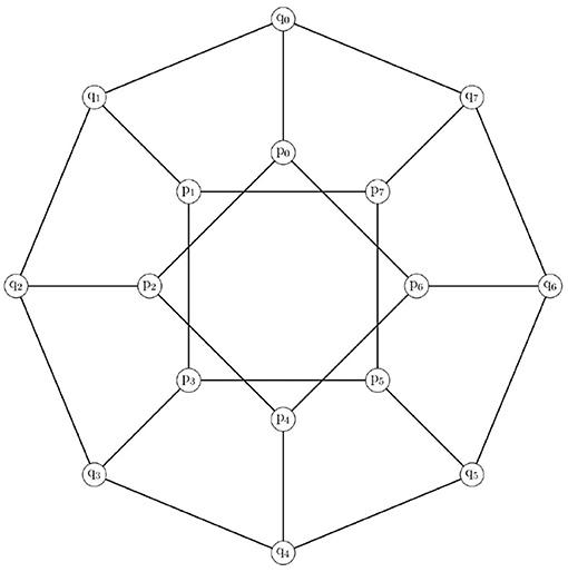
Figure 1. The generalized Petersen graph P(8, 2).
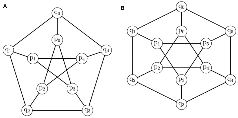
Figure 2. (A) The generalized Petersen graph P(5, 2), (B) The generalized Petersen graph P(6, 2).
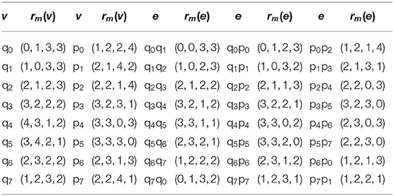
Table 1. Codes for P(n, 8).
The graph of the generalized Petersen graph comprises of three types of edges, external edges, internal edges, and spokes between qi and qi+1, pi and pi+m, and qi and pi, respectively. The vertices qi and pi (0 ≤ i ≤ n − 1) are termed as external and internal vertices, respectively.
The prism graph Dn is known as P(n, 1) for m = 1. Some of the already known results are given as
Theorem 1. [26] The metric dimension of , for n ≥ 4:
Theorem 2. [27] When, n ≥ 4, .
Theorem 3. [24] For n ≥ 5,
The known results for P(n, 2) concerning metric and an edge metric dimension are
Theorem 4. [28] For n ≥ 5, the metric dimension is β(P(n, 2)) = 3.
Theorem 5. [27] For n ≥ 5, βe(P(n, 2)) = 3.
It is quite natural to investigate the mixed metric dimension of P(n, 2). Now, we will find mixed the metric dimension of (P(n, 2)), and for this the following lemmas are presented.
Lemma 4. Case 1: If n ≡ 0(mod)4, then βm(P(n, 2)) ≤ 4.
Proof: The proof is n = 4r, r ≥ 4, where r ∈ ℤ+. The distinguishing vertices that will distinguish the whole vertices and edges of the graph are Rm = {q0, q1, p2r, p2r+1}. The following representations are presented with respect to Rm.
Representation of external vertices:
and,
Representation of internal vertices:
and,
Representation of external edges:
and,
Representation of external and internal edges:
and,
Representation of internal edges:
and,
□
Case 2: For n ≡ 2(mod)4, we have βm(P(n, 2) ≤ 4
Proof: Now we can see n = 4r + 2, r ≥ 4, where r ∈ ℤ+. The set of vertices that will distinguish the whole vertices and edges of the graph are Rm = {q0, q1, p2r+1, p2r+2}. The following representations are presented with respect to Rm.
Representation of external vertices:
and,
Representation of internal vertices:
and,
Representation of external edges:
and,
Representation of external and internal edges:
and,
Representation of internal edges:
and,
□
Now from lemma3, the resolving set Rm contains vertices from external and internal cycles; that is, the resolving set cannot comprise either external or internal vertices.
Lemma 5. When n ≡ 0, 2(mod4), then βm(P(n, 2)) ≥ 4.
Proof: Suppose that βm(P(n, 2)) = 3, the following contradictions arises:
Case 1: This is when the two fixed vertices are in the external cycle, {q0, q1}, and the other vertex lie in internal cycle pℓ, that is, Rm = {q0, q1, pℓ}.
(i) If 0 ≤ ℓ ≤ 1 then, rm{q0|q0, q1, pℓ} = rm{q0qn−1|q0, q1, pℓ} = (0, 1, ℓ + 1).
(ii) If ℓ = 2, 4, …, 2r, then rm{q0|q0, q1, pℓ} = rm{q0qn−1|q0, q1, pℓ}.
(iii) If ℓ = 3, 5, …, 2r−1, then rm{q0|q0, q1, pℓ} = rm{q0qn−1|q0, q1, pℓ}.
Case 2: When internal cycle contains two fixed vertices that is {p0, p1}, and the other vertex lie in external cycle qℓ. That is Rm = {p0, p1, qℓ}.
(i) If 0 ≤ ℓ ≤ 3, then rm{q0|p0, p1, qℓ} = rm{q0qn−1|p0, p1, qℓ} = (1, 2, ℓ).
(ii) If ℓ = 4, 6, …, 2r, then rm{q0|p0, p1, qℓ} = rm{q0qn−1|p0, p1, qℓ}.
(iii)If ℓ = 5, then rm{q0|p0, p1, qℓ} = rm{q0qn−1|p0, p1, qℓ} = (1, 2, ℓ).
(iv) If ℓ = 7, 9, …, 4r − 1, then rm{q1|p0, p1, qℓ} = rm{q1q2|p0, p1, qℓ}.
Similarly, other contradictions can be assumed; all the cases mentioned above suggest that βm(P(n, 2)) ≥ 4, which clearly indicates that βm(P(n, 2)) = 4 for n ≡ 0(mod4). Similar kind of contradictions can be proved for n ≡ 2(mod4). □
Remark 3: From the above cases, it can be deduced that if the mixed metric generator Rm for P(n, 2) contains two vertices of one cycle, then Rm contain at least two vertices of another cycle.
Lemma 6. βm(P(n, 2) ≤ 5, for n ≡ 1(mod)4
Proof: Case 1: Now we can write, if n = 4r + 1, r ≥ 4, where r ∈ ℤ+. The set of vertices that will distinguish the whole vertices and the edges of the graph are Rm = {q0, q1, p1, p2r+1, p2r+2}. The following representations are presented with respect to Rm.
Representation of external vertices:
and,
Representation of internal vertices:
and,
Representation of external edges:
and,
Representation of external and internal edges:
and,
Representation of internal edges:
and,
□
Proof: Case 2: Now we can write, if n = 4r + 3, r ≥ 4, where r ∈ ℤ+. The set of vertices which will distinguish the whole vertices, and edges of graph are Rm = {q0, q1, p1, p2r+3, p2r+4}. The following representations are presented with respect to Rm.
Representation of external vertices:
and,
Representation of internal vertices:
and,
Representation of external edges:
and,
Representation of external and internal edges:
and,
Representation of internal edges:
and,
□
Now, from lemma3, the resolving set Rm must contain vertices from both the external and internal cycles of graph.
Lemma 7. Suppose n ≡ 1, 3(mod4), then βm ≥ 5.
Proof: Suppose that βm = 4. If so, the following contradictions are assumed.
Case 1: When the external cycle contain three fixed vertices, {q0, q1, q2}, and other vertex lie in the internal cycle pℓ.
(i) If ℓ = 0, 2, 4, …, 2r, then rm{q0|q0, q1, q2, pℓ} = rm{q0qn−1|q0, q1, q2, pℓ} = (0, 1, 2, ℓ + 1).
(ii) If ℓ = 1, 3, 5, …, 4r − 1, then rm{q0|q0, q1, q2, pℓ} = rm{q0qn−1|q0, q1, q2, pℓ}.
Case 2: When {p0, p1, p2} lie in the internal cycle and the other vertex lie in the external cycle qℓ.
(i) If ℓ = 0, 2, 4, …, 2r, then rm{q0|p0, p1, p2, qℓ} = rm{q0qn−1|p0, p1, p2, qℓ}.
(ii) If ℓ = 1, 3, 5, …, 2r + 3, then rm{q0|p0, p1, p2, qℓ} = rm{q0qn−1|p0, p1, p2, qℓ}.
We already proved that for n ≡ 1, 3(mod4), and the mixed metric dimension is βm ≤ 5. From Remark2, we consider the following cases where the external and internal cycles comprise two vertices each.
Case 3: When two external vertices are fixed {q0, q1}, and the internal vertices are {p0, pℓ}.
(i) If ℓ = 0, 2, 4, …, 2r, then rm{q0|q0, q1, p0, pℓ} = rm{q0qn−1|q0, q1, p0, pℓ}.
(ii) If ℓ = 1, 3, 5, …, 4r − 1, then rm{q0|q0, q1, p0, pℓ} = rm{q0qn−1|q0, q1, p0, pℓ}.
Because of the symmetry, other possible cases can also be derived. From all the above cases, therefore, it is proven that, for n ≡ 1, 3(mod4), the mixed metric dimension is βm ≥ 5. We can therefore say βm = 5 when n ≡ 1, 3(mod4). □
Theorem 6. For n ≥ 7, we have a mixed metric dimension
Proof:Case 1: When n ≡ 0, 2(mod4).
From lemma 4,5, we have βmP(n, 2) = 4.
Case 1: When n ≡ 1, 3(mod4).
From lemma 6,7, we have βmP(n, 2) = 5. □
For the remainder of the cases, when n ≤ 15, the mixed metric dimension βm(P(n, 2)) is calculated through the total enumeration method, shown in Table 2, along with the mixed metric basis.
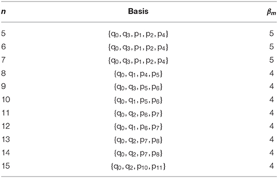
Table 2. Mixed Metric generator βm for P(n, 2).
The recently introduced mixed metric dimension is calculated for P(n, 2). It has been shown that P(n, 2) has mixed metric dimension equal to 4 for n ≡ 0, 2(mod4), and, for n ≡ 1, 3(mod4), the mixed metric dimension is 5. This shows that each graph of the family of generalized Petersen P(n, 2) has constant mixed metric dimension.
Theorem 7. [29] For the graph of P(n, 3),
and,
Theorem 8. [30] For n ≥ 17, we have,
Theorem 9. [31] The metric dimension of graph of P(2n, n) is
The standard metric dimension is examined for these as well as other known classes of generalized Petersen graphs; the mixed metric dimension for these as well as other graphs would therefore be intriguing to investigate. If the other variants of dimension are identified, a comparative study can be carried out; this could evaluate the relationship between β(Γ), βe(Γ), and βm(Γ) in the different families of graphs.
The original contributions presented in the study are included in the article/supplementary materials, further inquiries can be directed to the corresponding author/s.
The main idea was presented by HR. YJ read and approved the final manuscript.
The work of HR was supported by Post-Doctoral fund of University of Shanghai for Science and Technology under the grant no. 5B19303001. The work of YJ was supported by the National Science Foundation of China under grant no. 71571055.
The authors declare that the research was conducted in the absence of any commercial or financial relationships that could be construed as a potential conflict of interest.
We would like to express our sincere gratitude to the referees for a very careful reading of this paper and for all their insightful comments/criticism, which have led to a number of significant improvements to this paper.
1. Khuller S, Raghavachari B, Rosenfeld A. Landmarks in graphs. Discrete Appl Math. (1996) 70:217–29. doi: 10.1016/0166-218X(95)00106-2
4. Chartrand G, Saenpholphat V, Zhang P. The independent resolving number of a graph. Math Bohem. (2003) 128:379–93. Available online at: http://dml.cz/dmlcz/134003
5. Okamoto F, Phinezy B, Zhang P. The local metric dimension of a graph. Math Bohem. (2010) 135:239–55. Available online at: http://dml.cz/dmlcz/140702
6. Sebǒ A, Tannier E. On metric generators of graph. Math Oper Res. (2004) 29:383–93. doi: 10.1287/moor.1030.0070
7. Oellermann OR, Peters-Fransen J. The strong metric dimension of graphs and digraphs. Discrete Appl Math. (2007) 155:356–64. doi: 10.1016/j.dam.2006.06.009
8. Trujillo-Rasua R, Yero IG. k-Metric antidimension: a privacy measure for social graphs. Inform Sci. (2016) 328:403–17. doi: 10.1016/j.ins.2015.08.048
9. Shao Z, Wu P, Zhu E, Chen L. On metric dimension in some hex derived networks. Sensors. (2019) 19:94. doi: 10.3390/s19010094
10. Raza H, Hayat S, Imran M, Pan XF. Fault-tolerant resolvability and extremal structures of graphs. Mathematics. (2019) 7:78. doi: 10.3390/math7010078
11. Raza H, Hayat S, Pan XF. Binary locating-dominating sets in rotationally-symmetric convex polytopes. Symmetry. (2018) 10:727. doi: 10.3390/sym10120727
12. Raza H, Hayat S, Pan XF. On the fault-tolerant metric dimension of certain interconnection networks. J Appl Math Comput. (2019) 60:517–35. doi: 10.1007/s12190-018-01225-y
13. Raza H, Hayat S, Pan XF. On the fault-tolerant metric dimension of convex polytopes. Appl Math Comput. (2018) 339:172–85. doi: 10.1016/j.amc.2018.07.010
14. Kelenc A, Tratnik N, Yero IG. Uniquely identifying the edges of a graph: the edge metric dimension. Discrete Appl Math. (2018) 251:204–20. doi: 10.1016/j.dam.2018.05.052
15. Zubrilina N. On the edge dimension of a graph. Discrete Math. (2018) 341:2083–8. doi: 10.1016/j.disc.2018.04.010
16. Peterin I, Yero IG. Edge metric dimension of some graph operations. Bull Malay Math Sci Soc. (2019) 43:2465–77. doi: 10.1007/s40840-019-00816-7
17. Zhu E, Taranenko A, Shao Z, Xu J. On graphs with the maximum edge metric dimension. Discrete Appl Math. (2019) 257:317–24. doi: 10.1016/j.dam.2018.08.031
18. Liu JB, Wang C, Wang S, Wei B. Zagreb indices and multiplicative Zagreb indices of Eulerian graphs. Bull Malay Math Sci Soc. (2019) 42:67–78. doi: 10.1007/s40840-017-0463-2
19. Liu JB, Zhao J, Zhu Z. On the number of spanning trees and normalized Laplacian of linear octagonal quadrilateral networks. Int J Quantum Chem. (2019) 119:e25971. doi: 10.1002/qua.25971
20. Liu JB, Zhao J, Min J, Cao J. The hosoya index of graphs formed by a fractal graph. Fractals. (2019) 27:1950135–875. doi: 10.1142/S0218348X19501354
21. Liu JB, Zhao J, Cai ZQ. On the generalized adjacency, Laplacian and signless Laplacian spectra of the weighted edge corona networks. Phys A Stat Mech Appl. (2020) 540:123073. doi: 10.1016/j.physa.2019.123073
22. Liu JB, Shi ZY, Pan YH, Cao J, Abdel-Aty M, Al-Juboori U. Computing the Laplacian spectrum of linear octagonal-quadrilateral networks and its applications. Polycycl Aromat Compd. (2020). doi: 10.1080/10406638.2020.1748666. [Epub ahead of print].
23. Kelenc A, Kuziak D, Taranenko A, Yero IG. Mixed metric dimension of graphs. Appl Math Comput. (2017) 314:429–38. doi: 10.1016/j.amc.2017.07.027
24. Raza H, Liu JB, Qu S. On mixed metric dimension of rotationally symmetric graphs. IEEE Access. (2019) 8:11560–9. doi: 10.1109/ACCESS.2019.2961191
25. Watkins ME. A theorem on Tait colorings with an application to the generalized Petersen graphs. J Combinat Theory. (1969) 6:152–64. doi: 10.1016/S0021-9800(69)80116-X
26. Cáceres J, Hernando C, Mora M, Pelayo IM, Puertas ML, Seara C, Wood DR. On the metric dimension of cartesian products of graphs. SIAM J Discrete Math. (2007) 21:423–41. doi: 10.1137/050641867
27. Filipović V, Kartelj A, Kratica J. Edge metric dimension of some generalized petersen graphs. Results Math. (2019) 74:182. doi: 10.1007/s00025-019-1105-9
28. Javaid I, Rahim MT, Ali K. Families of regular graphs with constant metric dimension. Utilitas Math. (2008) 75:21–34.
29. Imran M, Baig AQ, Shafiq MK, Tomescu I. On metric dimension of generalized petersen graphs P (n, 3). Ars Comb. (2014) 117:113–30.
30. Naz S, Salman M, Ali U, Javaid I, Bokhary SA. On the constant metric dimension of generalized Petersen graphs P (n, 4). Acta Math Sin. (2014) 30:1145–60. doi: 10.1007/s10114-014-2372-8
Keywords: mixed metric dimension, metric dimension, edge metric dimension, generalized Petersen graph, exact values
Citation: Raza H and Ji Y (2020) Computing the Mixed Metric Dimension of a Generalized Petersen Graph P(n, 2). Front. Phys. 8:211. doi: 10.3389/fphy.2020.00211
Received: 09 April 2020; Accepted: 18 May 2020;
Published: 28 July 2020.
Edited by:
Shaohui Wang, Louisiana College, United StatesReviewed by:
Muhammad Kamran Siddiqui, COMSATS University Islamabad, Lahore Campus, PakistanCopyright © 2020 Raza and Ji. This is an open-access article distributed under the terms of the Creative Commons Attribution License (CC BY). The use, distribution or reproduction in other forums is permitted, provided the original author(s) and the copyright owner(s) are credited and that the original publication in this journal is cited, in accordance with accepted academic practice. No use, distribution or reproduction is permitted which does not comply with these terms.
*Correspondence: Ying Ji, aml5aW5nQHVzc3QuZWR1LmNu
Disclaimer: All claims expressed in this article are solely those of the authors and do not necessarily represent those of their affiliated organizations, or those of the publisher, the editors and the reviewers. Any product that may be evaluated in this article or claim that may be made by its manufacturer is not guaranteed or endorsed by the publisher.
Research integrity at Frontiers
Learn more about the work of our research integrity team to safeguard the quality of each article we publish.