 William Scott Raburn
 Greg Gbur
- Department of Physics and Optical Science, University of North Carolina at Charlotte, Charlotte, NC, United States
Singularities in the polarization state of non-uniform electromagnetic beams have been a topic of both theoretical and practical interest for many years, as have singularities in the correlation functions of random scalar wavefields. However, there has been relatively little work done to explore the intersection of these phenomena, namely singularities in the polarization state of partially coherent wavefields. In this paper, we use a simple model of a partially coherent electromagnetic vortex beam to highlight three different ways that one can define polarization singularities in scalar wavefields, one of which has been previously undiscussed.
1. Introduction
The study and application of singularities in wavefields has grown in recent years into a vibrant and significant subfield of optics, known as singular optics [1–3]. The most commonly discussed types of such singularities are phase singularities in scalar waves, which typically manifest as lines of zero intensity in three-dimensional space. Around these singularities the phase has a circulating or helical structure, which has led to them being called optical vortices, here referred to as scalar optical vortices. Such singularities have been applied to fields, such as free-space optical communication [4, 5], optical tweezing [6, 7], and image processing [8, 9].
To use a scalar wave description of light, the state of polarization is assumed to be uniform. Research over the past 20 years has demonstrated, however, that novel effects arise for optical beams that have spatially-varying polarization, known as vector beams. For vector beams, singularities of phase are no longer typical, and instead the most common singularities are singularities of the state of polarization. These come in two generic types: C-points (points of circular polarization where the orientation of the polarization ellipse is undefined) and L-lines (lines of linear polarization where the helicity of the polarization ellipse is undefined). Much work has been done to elucidate the properties of polarization singularities, and beams with such singularities have been shown to be useful in a number of applications, including focusing [10, 11] and atmospheric propagation [12, 13].
But no light wave is truly monochromatic, and in recent years researchers have delved into the behavior of wavefield singularities when the field is partially coherent. For the scalar case, it has been shown that phase singularities evolve into singularities of the two-point correlation function when the spatial coherence of a wavefield is decreased [14–16]. There has now been a significant amount of research on partially coherent scalar vortex beams [17–20].
In contrast, there has been relatively little work done to investigate the nature of polarization singularities in partially coherent vector vortex beams, and how they are related to their fully coherent counterparts; exceptions include the papers of Felde et al. [21], and Soskin and Polyanskii [22]. The vectorial nature of such beams, however, presents more than one way to define singularities related to the state of polarization In this paper, we highlight three ways of characterizing the singularities of a partially coherent electromagnetic wavefield, one of which has previously gone unmentioned. We introduce a simple model of a partially coherent electromagnetic beam possessing a polarization singularity, and examine how that polarization singularity manifests through the different ways of characterizing it.
We begin by reviewing needed definitions related to polarization singularities and coherence, and then discuss the different ways of classifying singularities in partially coherent electromagnetic waves. We then use our model to examine the relationships between the different classifications, and their significance.
2. Polarization Singularities
In a coherent paraxial electromagnetic wave, the state of polarization is generally elliptical, with the polarization ellipse described by its handedness, angle of orientation Ψ, and ellipticity (ratio of minor to major axis). The most commonly occurring, or generic, singularities in the cross-section of such a beam are C-points and L-lines, which correspond to points of circular polarization and lines of linear polarization, respectively. C-points are singularities in the orientation of the polarization ellipse, and L-lines are singularities in the handedness of the ellipse. We focus on C-points and their non-generic cousins here, which are the most topologically interesting.
C-points may be readily found using the Jones vector of the electric field in a circular polarization basis, which we write as |E〉LR. Here “LR” refers to the left-hand circular EL and right-hand circular ER complex components of the electric field, with vector dependencies and , respectively. A point of pure circular polarization will manifest anywhere that one of the complex components vanishes, e.g., EL = 0. The phase θL of the component at this point is consequently undefined, making, for example, a right-handed C-point a phase singularity of the scalar component EL of the field.
C-points are characterized by the behavior of the orientation angle Ψ as one traverses a closed loop around the singular point. This angle must vary continuously with position, except at the C-point itself, and therefore can only change by multiples of 180° around any closed loop. This change is referred to as the topological index n, and may be formally defined by the following integral,
The topological index of different polarization singularities is additive: a loop taken around multiple singularities will give an index equal to the sum of the indices of the individual singularities. C-points in particular come in three generic types: lemons with index n = +1/2, stars with index n = −1/2, and monstars with index n = +1/2. The monstar is a less common transition singularity formed in creation and annihilation events between singularities, so we focus on lemons and stars, which are illustrated in Figure 1. In this figure, we illustrate the orientation of the major axis with line segments as well as colors representing the angles.
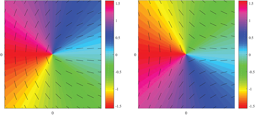
Figure 1. Orientation of the major axis of the polarization ellipse for (left) a lemon (n = 1/2) and (right) a star (n = −1/2), in the plane perpendicular to the optical axis. The major axis is depicted two ways: with lines indicating the major axis direction for selected positions and with a colormap to indicate the value of Ψ.
It is to be noted that the topological index can be readily found from the values of the topological charges of the two components EL and ER of the electric field, as we now show. The topological charge t is the net number of 2π changes the phase of the component undergoes in a closed path around the singularity or singularities, and is formally defined as
where θ is the phase of the particular component.
To determine the relation between the charges of the components and the index of the singularity, we apply some intuition about the properties of the polarization ellipse. In the LR basis, the two vector components rotate in opposite directions with angles that we label as ϕL(r, t), ϕR(r, t). The total field will point along the major axis of the ellipse at a time t0 when these two angles correspond with the ellipse orientation angle, or
But these two rotation angles may be related to the complex phases θL,R(r) by the relations
where ω is the angular frequency of light. We may eliminate the time dependence t0 from these equations by summing ϕL(r, t) and ϕR(r, t); by further using Equation (3), we get the relation
If we substitute this expression into Equation (1), we readily find that
Using the definition of topological charge, we have
In short, the topological index can be determined directly from the difference of the enclosed topological charges of the left- and right-handed components; this result was first determined by Angelsky et al. [23].
It is to be noted that this result indicates that polarization singularities of topological index n = ±1/2 can come in generic and non-generic forms. In the generic form, one component has topological charge unity and the other has topological charge zero, resulting in a point of circular polarization, and the C-points are the types one expects to see form naturally in random wavefields. However, any case where the topological charges differ by an integer will result in a half-integer topological index, and will have the form of a star or lemon. However, the intensity of the field will be zero at the singularity, and not a point of circular polarization. We refer to these non-generic lemons and stars as polarization vortices to distinguish them from C-points.
3. Partial Coherence in Scalar and Vector Fields
The discussion so far has focused on monochromatic fields. When studying fields that are fluctuating in space and time, one must turn to a statistical description of their behavior. For scalar fields, the preferred quantity of study is the cross-spectral density; for vector fields, the preferred quantity is the cross-spectral density matrix. In this section we briefly review relevant definitions related to these functions.
For a statistically stationary scalar field, the cross-spectral density W(r1, r2, ω) of the field at two points r1 and r2 may be defined as
where we use a tilde to represent the complex conjugate and 〈⋯ 〉ω represents an average over an ensemble of monochromatic fields {U(r, ω)}; as first demonstrated by Wolf [24], this ensemble can be created for any partially coherent field. The cross-spectral density is in general frequency dependent, but for quasi-monochromatic fields of central frequency ω0 the overall behavior of the field can be well-represented by the cross-spectral density evaluated at ω0; we will consider such cases for simplicity and suppress the frequency dependence in later expressions.
The cross spectral density can be used to directly calculate two important observables of the field: the spectral density S(r) = W(r, r) and the spectral degree of coherence μ(r1, r2), a normalized quantity that is equal to the visibility of interference fringes observed when measured with Young's two-pinhole experiment,
As also shown by Wolf [24], the cross-spectral density can always be written in a modal representation called the coherent mode representation, of the form
Here, λs ≥ 0 is an eigenvalue and ϕs(r) is an orthonormal eigenfunction of the cross-spectral density, as determined from the relation
The domain of integration depends on the geometry of the problem, but is typically taken to be the source plane of a paraxial beam. The summation may be over one or more indices, and may be finite or infinite; for a two-dimensional domain, it is typically a double sum.
The coherent mode representation is a convenient way to illustrate that singularities of phase—associated with zeros of intensity—are not typical features of partially coherent waves. As first noted in reference [14], in order for a zero of intensity to appear at a given point, the real and imaginary parts of each mode must simultaneously vanish at that point. If there are N modes, this involves satisfying 2N equations with 2 degrees of freedom in a cross-section of the partially coherent beam. This is an overspecified problem unless N = 1, which is the fully coherent case. So phase singularities associated with zeros of intensity are not commonly encountered in partially coherent fields.
Phase singularities of two point correlation functions, such as the cross-spectral density, however, are common. The cross-spectral density satisfies a pair of Helmholtz equations, and by fixing one point, say , the cross-spectral density is equivalent to a monochromatic wave in the other variable, satisfying the Helmholtz equation,
where k = ω/c and is the Laplacian with respect to variable r2. Just as monochromatic fields will typically possess optical vortices, the cross-spectral density will typically possess coherence vortices. It is to be noted, however, that by fixing one point of observation, we are only seeing a projection of the singularity, which exists in a higher-dimensional r1, r2 space; studies of the structure of the complete singularity have been done in both the source plane [16] and on propagation [25].
For convenience, we note that the cross-spectral density may be written using bra-ket notation from quantum theory,
where 〈r|s〉ω = ϕs(r, ω) and λ is equivalent to the usual quantum density operator.
When studying paraxial electromagnetic beams, it is most efficient to decompose them into two orthogonal polarization components and . Therefore, there are four different field correlations to consider, between 4 different scalar modes Ea(r1), Ea(r2), Eb(r1), and Eb(r2). In order to deal with this increased complexity, the cross spectral density matrix is introduced,
A number of observables of the field may be calculated from this matrix, such as the polarization matrix and the electromagnetic degree of coherence [26], defined as
where Tr represents the trace of the matrix. In analogy with the scalar cross-spectral density, can be written in a coherent mode representation.
or in terms of the density operator
where now 〈s|r1 〉 = Es(r1) represents a vector coherent mode of the field.
4. Singularities in Partially Coherent Vector Beams
In making a change from scalar beams to vector beams, the singularities of interest change from optical vortices to polarization singularities. In making a change from coherent scalar beams to partially coherent scalar beams, the singularities of interest change from optical vortices to correlation vortices. We now come to the key observation of this article: in going from coherent vector beams to partially coherent vector beams, we end up with more than one way of defining and characterizing the singularities. In this section, we first discuss two known ways of characterizing them and then introduce a third.
The first approach is perhaps the most straightforward: at any given point, i.e., r1 = r2 ≡ r, we may always uniquely decompose the cross-spectral density into a fully polarized part and a completely unpolarized part, as first illustrated by Stokes [27] and derived in modern form in reference [28]. The polarized part by itself will be a continuous vector field, and will therefore possess C-points that can be characterized as for a fully coherent field, which we refer to as coherent polarization singularities. The decomposition may be written in the form
The polarized and unpolarized parts may be written as
where
We may view this characterization of the singularities of the field as looking purely at their vector nature, by focusing on the “diagonal” (r1 = r2) elements of the cross-spectral density. This decomposition was originally formulated in the xy polarization basis, but has the same form in the LR basis.
Working in the LR basis has a particular advantage in studying singularities, however. Because a C-point is defined as a point where the field is circularly polarized, JLR = 0 at every C-point. Furthermore, the coherent part of the field can be written as the direct product of a Jones vector with itself in the LR basis, with components , , such that . Since Equation (5) shows that the orientation angle Ψ(r) is directly related to the phases of the LR field components through 2Ψ(r) = θR(r) − θL(r), the orientation angle of the ellipse for the coherent part of the field can be derived directly from the phase of JLR(r).
It is to be noted that this decomposition cannot be applied globally to the whole beam. As was shown by Wolf [29], it is not in general possible to separate a paraxial vector beam into a polarized beam and unpolarized beam, each of which individually satisfies the wave equation.
An alternative approach for studying the singularities of a vector cross-spectral density is to focus on the analogy with the scalar case, and look for coherence singularities in the directly observable part of the vector field. When performing Young's two-pinhole experiment with partially coherent electromagnetic waves, the visibility of interference fringes is given by η(r1, r2), defined in Equation (15). In analogy with the scalar case, we may find eta singularities by fixing one observation point and looking for singularities with respect to the second point r2, i.e., points where . As noted by Raghunathan et al. [30, 31], these singularities behave like scalar coherence vortices, with a discrete topological charge. Eta singularities have been relatively unexplored compared to other classes of singularities, though they have been observed in Mie scattering [32] and in the propagation of partially coherent radially polarized beams [33]. Whereas, the coherent polarization singularities focused on the diagonal elements of the cross-spectral density matrix in space (r1 = r2), this representation looks at the diagonal elements with respect to polarization, in the form of the trace.
There is a third option, however, that may in a sense be considered a hybrid of the two, or even a generalization. As in the scalar case, we look at the projection of the cross-spectral density on a fixed reference point . Doing that here leaves us with a quantity that depends on a single spatial variable r2, but is still a 2 × 2 matrix. We now further contract the cross-spectral density matrix with a polarization state as well.
The resultant quantity is a non-uniform complex vector field, which we expect to possess polarization singularities; we refer to these as partially coherent polarization singularities. Whereas, the two previous classes of singularities essentially simplified the cross-spectral density matrix by diagonalizing in either space or polarization and projecting with respect to the other quantity, here we perform a projection with respect to both space and polarization.
It is to be noted that the cross-spectral density matrix, and consequently the vector , are measured in the LR circular polarization basis. The resulting vector can be written in terms of L and R components as
Several questions arise upon seeing the variety of distinct types of singularities that can appear in partially coherent vector beams. The first of these is: how are such singularities related to the singularities of the field in the coherent limit, if at all? The second question is: what is the significance of these different types of singularities? In the next section, we introduce a simple model of a partially coherent vector beam with controllable spatial coherence to answer these questions.
5. Construction of Model PC Beams
To construct a model of a partially coherent beam with a built-in polarization singularity, we will utilize the relationship (7) between topological index and topological charge in the LR polarization basis to first construct a coherent field possessing polarization singularities. This field will then be used in a beam wander model to produce the cross-spectral density matrix of a partially coherent non-uniformly polarized beam. The behavior of the beam's singularities can then be analyzed as a function of the spatial coherence.
To model the R and L components of the coherent beam, we will use Laguerre-Gauss beams of radial order 0 and azimuthal order m; we write these modes as |m〉. We write the particular orders of each component as m = tR and m = tL.
Written in coordinates natural for vortex beams, r± = x ± iy, and using t = αm where α = ±1, the field of a scalar component with singularity centered at c = (c+, c−) is, in bra-ket notation,
The complex scalar constant ; from this we can determine the beam width w2(z) = 2|σ2(z)|/cos(Φ(z)) and the Gouy phase, Φ = arg(σ2). The fields are taken to be normalized; the normalization factors are included in
Equation (27) describes the behavior of a scalar field at any propagation distance z. An electromagnetic field built from the scalar modes |c, t〉 may then be written as
To summarize the notation: here ti represents the topological charge of the ith component, where αi is its sign and mi is its magnitude.
Using this model, a coherent beam of n = 1/2, for example, could be constructed with (tR, tL) = (m + 1, m) for any integer m. The λi in the model are complex coefficients whose relative phase affects the orientation of the polarization singularity, and whose magnitudes define how far from the polarization singularity an L-line will manifest. However, the location of singularities in the cross spectral density matrix will be affected by the particular choice made, so they will be taken to both be unity for the remainder of this article.
The beam wander model is a construction of a partially coherent beam through an ensemble of coherent beams with shifted central axes. This model was first used in 2004 [14] to model a partially coherent scalar vortex beam, and may now be considered a special case of a technique for designing genuine correlation functions [34]. The transverse position of the central axis is defined by the central point c and the probability density of the ensemble is given by ρ(c). For a scalar beam Φ(r − c), the cross-spectral density has the form
The probability density is usually taken to be of Gaussian form, which allows the entire integral to be evaluated analytically.
To create a polarization vortex beam with a prescribed topological index, it is convenient to use separate phase vortex solutions for the R and L components and take advantage of the relationship of their topological charges to index n described in Equation (7). A scalar model of partially coherent Gaussian beams of arbitrary topological charge was introduced by Stahl and Gbur [20], and can be used to apply the beam wander model to the R and L components. To make partially coherent beams carrying lemons and stars, we will expand that model to the electromagnetic case and then choose the azimuthal modes of the L and R components so that .
The result is the following expression for the cross-spectral density matrix,
with probability density
Here δ represents the amount of wander the beam undergoes; δ = 0 represents the coherent limit.
The diagonal terms for this have already been solved in Stahl and Gbur [20], giving
In this expression, Wg is a Gaussian term dependent on the widths of the mode and the probability density function, Qij is a coefficient dependent on the topological charges ti = αimi,
and Hi is a complex function that depends on the two coordinates r and rP of the cross-spectral density,
Furthermore, Δ is a length parameter of the form,
It is to be noted that the function Wg possesses no zeros and therefore does not affect the number of singularities or their positions for any of the singularity types considered.
The off-diagonal components of the cross spectral density matrix may be solved in a similar manner, by evaluating the integral,
Following a procedure analogous to that of reference [20], we employ the substitution , together with binomial expansions of the vortex terms to get the following expression for the off-diagonal elements of ,
The integral over ϕ is equal to 2πδαjl − αik, applying this and a straightforward Gaussian integral compresses our result to the form,
where Pij is a polynomial factorable into r+ and r− terms and mmin is the minimum of {mi, mj}. Using this formula, we can write the cross-spectral vectors, defined in Equation (25), and electromagnetic degree of coherence, defined in Equation (15), in terms of the non-zero Wg and the polynomials Pij in the form
Because our expression for the cross-spectral density matrix is analytic, we can directly determine the number of phase singularities each component must possess. Referring to Equation (39) for Pij, we see that the largest powers of the polynomial are of the forms and , resulting in mi and mj distinct roots, respectively. We may therefore expect that there will be mi first-order singularities of charge −αi, and mj first-order singularities of charge +αj.
We may use this observation to determine the singular behavior of the beam for each type of singularity discussed. For coherent polarization singularities, the net topological index, given by Equation (7), will be determined by the zeros of WLR, or
The topological index of the coherent part of the beam will therefore remain constant, regardless of the state of coherence.
For eta singularities, we combine Wii and Wjj. The first term will be a polynomial of order mi in both +αi and −αi, and the second term will be a polynomial of order mj in both +αj and −αj. Let us consider the case where both αi > 0 and αj > 0, for simplicity. Because the order of a sum of polynomials is the maximum of the orders of the individual polynomials, we find that the number of positive singularities and negative singularities is given by
The net topological charge will always be zero, though the number of positive and negative charges will depend on the order of the components. For example, a lemon made from tR = 3 and tL = 2 would have 3 pairs of t = 1 and t = −1 phase vortices.
A similar calculation may be done to determine the number and type of singularities in . We again restrict ourselves to the case where αi > 0 and αj > 0. In this case, the left component of the vector will have max(mR, mL) negative charges and mL positive charges in general, while the right component of the vector will have mR positive charges and max(mR, mL) negative charges. The total number of lemons and stars may then be calculated by:
This assumes that none of the zeros coincide, which is the typical scenario. It is to be noted that the number may change in the special case when the projection vector is taken to be a pure circular polarization state. By making an appropriate selection of , not only the positions of the polarization singularities but their total number may therefore be manipulated.
6. Singularities in Model Beams
We may now apply our model to investigate and confirm the behavior of the three classes of singularities for partially coherent electromagnetic beams and their relationships to the underlying singularity of the coherent beam. In all examples, we take w0 = 0.5cm.
We first consider the case of coherent polarization singularities, characterized by points where JLR(r) = 0, where we take tR = 1, tL = 0, resulting in a generic lemon. Figure 2 shows the behavior of the polarization singularity as the spatial coherence is decreased.
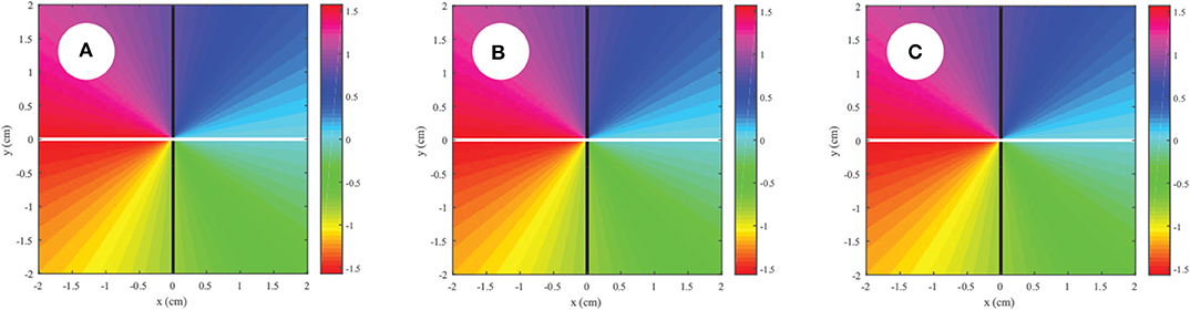
Figure 2. Behavior of a coherent polarization singularity as the spatial coherence is decreased, with (A) δ = 0.1cm, (B) δ = 0.5cm, (C) δ = 3cm.
It can be seen that the singularity is unchanged in position or even in phase structure as δ is varied. This result is also true for a non-generic lemon, with tR = 3 and tL = 2 (not shown). We may explain this result as arising from the rotational symmetry of all constituent parts of the field: the left and right components of the field, as well as the probability distribution ρ(c), are all symmetric about their central axes. Therefore, there is nothing in the model that provides a direction to break symmetry and allow the position of the polarization singularity to change. This result is noteworthy as it suggests that the coherent polarization singularities maintain their original structure when a beam is randomized under quite general circumstances, and indicates that the topological index will remain unchanged on randomization, as predicted by Equation (42).
The situation for eta singularities, where η(rP, r) = 0, is significantly different. In Figure 3, there is no eta singularity at the origin in the coherent limit, whereas there is a polarization singularity at that position. This discrepancy arises because eta singularities are associated with a zero of , which typically evolves into a zero of intensity in the coherent limit. A generic C-point has a non-zero intensity, so this polarization singularity is not directly reflected in the behavior of the eta singularities.
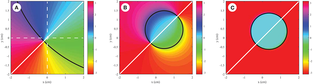
Figure 3. Behavior of an eta singularity as the spatial coherence is decreased, with (A) δ = 0.1cm, (B) δ = 0.5cm, (C) δ = 3cm. Here tR = 1, tL = 0 and the observation point is taken at r1 = (0.35, 0.35)cm. Dashed lines have been included to show the position of the coordinate system origin.
It can be seen that, as the spatial coherence is decreased, a second eta singularity of opposite charge approaches from the point at infinity along the line of r1, resulting in a field with a net topological charge of zero near the origin. This is the same behavior seen for correlation singularities in scalar fields [14].
For a non-generic polarization vortex, the eta singularity behavior connects more closely to the underlying polarization singularity, as seen in Figure 4. In the coherent limit, the polarization singularity is also a point of zero intensity due to the overlap of zeros of the L and R components of the field. Therefore, this corresponds to an eta singularity at the origin, and that eta singularity is preserved as the spatial coherence is decreased.
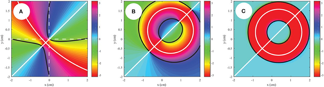
Figure 4. Behavior of an eta singularity as the spatial coherence is decreased, with (A) δ = 0.1cm, (B) δ = 0.5cm, (C) δ = 3cm. Here tR = 2, tL = 1 and the observation point is taken at . Dashed lines have been included to show the position of the coordinate system origin.
In Figure 3, we end up with a single plus-minus pair as coherence is decreased, whereas in Figure 4 we end up with three pairs. These results are consistent with the predictions of Equation (43).
We finally consider the behavior of partially coherent polarization singularities where , where the behavior of such singularities strongly depend on the choice of projection . We may naturally decompose the behavior into the case where is parallel to the polarized part of the field at the observation point rP and the case where is perpendicular to this polarized part. Figure 5 shows the parallel case; we can see that, in the coherent limit, this projection accurately reproduces the lemon behavior at the origin.
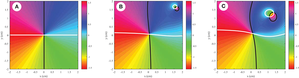
Figure 5. Behavior of a partially coherent polarization singularity as the spatial coherence is decreased, with (A) δ = 0.1cm, (B) δ = 0.5cm, (C) δ = 3cm. Here tR = 1, tL = 0 and the observation point is taken at . The unit vector is taken parallel to the polarized part of the field at .
The situation is different for the perpendicular case, as shown in Figure 6. The net topological index stays equal to that of the coherent limit, but there are additional singularities present for this case, even as we approach full coherence.
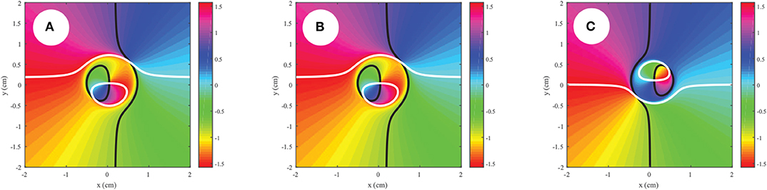
Figure 6. Behavior of a partially coherent polarization singularity as the spatial coherence is decreased, with (A) δ = 0.1cm, (B) δ = 0.5cm, (C) δ = 3cm. Here tR = 1, tL = 0 and the observation point is taken at r1 = (0.35, 0.35)cm. The unit vector is taken perpendicular to the polarized part of the field at .
According to Equation (45), we expect to see two lemons and one star in general in the projection as the coherence is decreased, and this is true in both Figures 5, 6. To further confirm that our calculation in Equation (45) is correct, we consider the higher-order polarization vortex case with tR = 2, tL = 1 in Figure 7. Now we predict 4 lemons and 3 stars, which can be seen in Figures 7C,D. It is to be recalled, however, that the number of zeros depends on the projection vector ; in our case, we find that annihilation events happen in Figure 7E, resulting in fewer singularities in the low coherence limit.
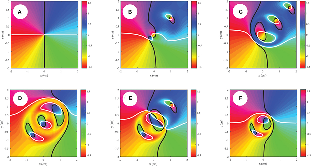
Figure 7. Behavior of a partially coherent polarization singularity as the spatial coherence is decreased, with (A,D) δ = 0.1cm, (B,E) δ = 0.5cm, (C,F) δ = 3cm. Here tR = 2, tL = 1 and the observation point is taken at r1 = (0.35, 0.35)cm. The unit vector is taken parallel to the polarized part of the field at in (A–C) and perpendicular in (D–F).
7. Conclusion
Although there is a simple relationship between coherent optical vortices and correlation singularities when looking at scalar wavefields, there are multiple ways to define singularities of a partially coherent vector field. In this article we have discussed three different methods for defining partially coherent vector singularities, and introduced a simple model of a partially coherent vector field to compare them.
Our model demonstrates that, in each case, the singularities that exist in a coherent vector field do evolve into singularities of the cross-spectral density matrix, though each of the partially coherent projections have different relationships to their coherent counterparts. It is to be noted that each of these projections will have their own relevance to experimental observations. The coherent polarization singularities will be reflected in the Stokes parameters of the partially coherent field, whereas the eta singularities and partially coherent polarization singularities will appear in Young's two-pinhole interference experiments, where the fields from two different spatial points are interfered. Furthermore, because the first two methods involve a diagonalized projection of the cross-spectral density matrix in space or polarization, partially coherent polarization singularities cannot be derived from measurements of either of these, and vice-versa. They represent distinct manifestations of singularities in the partially coherent vector case.
It is of interest to note that there is an analogy here to a discussion that arose several years ago, relating to the proper definition of the degree of coherence when dealing with electromagnetic fields. In addition to the aforementioned definition using eta [26], which is determined by the visibility of interference fringes, Tervo et al. [35] simultaneously introduced a definition that stresses the statistical correlations between field components. A third definition was introduced by Réfrégier and Goudail [36] that stresses invariant properties of the field. It appears that the appropriate choice of degree of coherence depends on the interests of the experimenter, and we expect the same is true for the multiple possible definitions of singularities in partially coherent electromagnetic fields.
This article focuses on several definitions of electromagnetic singularities. Like the scalar case [16], however, all these definitions are projections of the true partially coherent electromagnetic singularities which exist in a higher-dimensional space, and which is not easily visualized. Future work will involve trying to determine the nature of such singularities, and it is hoped that the recognition of the various projections will aid in this investigation.
From a practical perspective, we note that there has been much attention paid in recent years to the use of optical vortices in free-space optical communication, which potentially have several advantages over traditional communication schemes [4, 5]. With this in mind, it would seem that beams possessing vector singularities will be a natural next step in research, especially considering that vector beams possess some advantages over scalar beams on propagating in atmospheric turbulence [12]. An understanding of how polarization singularities evolve when the spatial coherence of beams is reduced will be essential for such research, and we hope that this paper is a step in that direction.
Data Availability Statement
The datasets generated for this study are available on request to the corresponding author.
Author Contributions
Both authors contributed equally to the work presented here. WR did theoretical calculations and derived the examples given, while GG did theoretical calculations and provided analysis of the results.
Funding
This work was funded by the Air Force Office of Scientific Research (AFOSR) (FA9550-16-1-0240).
Conflict of Interest
The authors declare that the research was conducted in the absence of any commercial or financial relationships that could be construed as a potential conflict of interest.
References
2. Dennis MR, O'Holleran K, Padgett MJ. Singular optics: optical vortices and polarization singularities. In: Wolf E, editor. Progress in Optics. Vol. 53. Amsterdam: Elsevier (2009). p. 293. doi: 10.1016/S0079-6638(08)00205-9
3. Soskin MS, Vasnetsov MV. Singular optics. In: Wolf E, editor. Progress in Optics. Vol. 42. Amsterdam: Elsevier (2001). p. 219. doi: 10.1016/S0079-6638(01)80018-4
4. Gibson G, Courtial J, Padgett MJ, Vasnetsov M, Pas'ko V, Barnett SM, et al. Free-space information transfer using light beams carrying orbital angular momentum. Opt Exp. (2004) 12:5448–56. doi: 10.1364/OPEX.12.005448
5. Wang J, Yang JY, Fazal IM, Ahmed N, Yan Y, Huang H, et al. Terabit free-space data transmission employing orbital angular momentum multiplexing. Nat Photon. (2012) 6:488–96. doi: 10.1038/nphoton.2012.138
6. Gahagan KT, Swartzlander GA. Optical vortex trapping of particles. Opt Lett. (1996) 21:827–9. doi: 10.1364/OL.21.000827
7. Simpson NB, Dholakia K, Allen L, Padgett MJ. Mechanical equivalence of spin and orbital angular momentum of light: an optical spanner. Opt Lett. (1997) 22:52–54. doi: 10.1364/OL.22.000052
8. Davis JA, McNamara DE, Cottrell DM, Campos J. Image processing with the radial Hilbert transform: theory and experiments. Opt Lett. (2000) 25:99–101. doi: 10.1364/OL.25.000099
9. Fürhapter S, Jesacher A, Bernet S, Ritsch-Marte M. Spiral phase contrast imaging in microscopy. Opt Exp. (2005) 13:689–94. doi: 10.1364/OPEX.13.000689
10. Youngworth KS, Brown TG. Focusing of high numerical aperture cylindrical vector beams. Opt Exp. (2000) 7:77–87. doi: 10.1364/OE.7.000077
11. Dorn R, Quabis S, Leuchs G. Sharper focus for a radially polarized light beam. Phys Rev Lett. (2003) 91:233901. doi: 10.1103/PhysRevLett.91.233901
12. Gu Y, Korotkova O, Gbur G. Scintillation of nonuniformly polarized beams in atmospheric turbulence. Opt Lett. (2009) 34:2261–3. doi: 10.1364/OL.34.002261
13. Wang F, Liu X, Liu L, Yuan Y, Cai Y. Experimental study of the scintillation index of a radially polarized beam with controllable spatial coherence. Appl Phys Lett. (2013) 103:091102. doi: 10.1063/1.4819202
14. Gbur G, Visser TD, Wolf E. ‘Hidden’ singularities in partially coherent fields. J Opt A. (2004) 6:S239–42. doi: 10.1088/1464-4258/6/5/017
15. Gbur G, Visser TD. Phase singularities and coherence vortices in linear optical systems. Opt Commun. (2006) 259:428–35. doi: 10.1016/j.optcom.2005.08.074
16. Gbur G, GA, Swartzlander J. Complete transverse representation of a correlation singularity of a partially coherent field. J Opt Soc Am B. (2008) 25:1422–9. doi: 10.1364/JOSAB.25.001422
17. Maleev ID, Palacios DM, Marathay AS, Swartzlander, Jr GA. Spatial correlation vortices in partially coherent light: theory. J Opt Soc Am B. (2004) 21:1895–900. doi: 10.1364/JOSAB.21.001895
18. Wang W, Duan Z, Hanson SG, Miyamoto Y, Takeda M. Experimental study of coherence vortices: local properties of phase singularities in a spatial coherence function. Phys Rev Lett. (2006) 96:073902. doi: 10.1103/PhysRevLett.96.073902
19. Yang Y, Chen M, Mazilu M, Mourka A, Liu YD, Dholakia K. Effect of the radial and azimuthal mode indices of a partially coherent vortex field upon a spatial correlation singularity. New J Phys. (2013) 15:113053. doi: 10.1088/1367-2630/15/11/113053
20. Stahl CSD, Gbur G. Partially coherent vortex beams of arbitrary order. J Opt Soc Am A. (2017) 34:1793–9. doi: 10.1364/JOSAA.34.001793
21. Felde CV, Chernyshov AA, Bogatyryova GV, Polyanskii PV, Soskin MS. Polarization singularities in partially coherent combined beams. JETP Lett. (2008) 88:418. doi: 10.1134/S002136400819003X
22. Soskin MS, Polyanskii PV. New polarization singularities of partially coherent light beams. Proc SPIE. (2010) 7613:76130G. doi: 10.1117/12.840197
23. Angelsky O, Mokhun A, Mokhun I, Soskin M. The relationship between topological characteristics of component vortices and polarization singularities. Opt Commun. (2002) 207:57–65. doi: 10.1016/S0030-4018(02)01479-7
24. Wolf E. New theory of partial coherence in the space-frequency domain. Part 1: spectra and cross-spectra of steady-state sources. J Opt Soc Am. (1982) 72:343–51. doi: 10.1364/JOSA.72.000343
25. Stahl CSD, Gbur G. Complete representation of a correlation singularity in a partially coherent beam. Opt Lett. (2014) 39:5985–8. doi: 10.1364/OL.39.005985
26. Wolf E. Unified theory of coherence and polarization of random electromagnetic beams. Phys Lett A. (2003) 312:263–7. doi: 10.1016/S0375-9601(03)00684-4
27. Stokes GG. On the composition and resolution of streams of polarized light from different sources. Trans Camb Phil Soc. (1852) 9:399–416.
28. Wolf E. Introduction to the Theory of Coherence and Polarization of Light. Cambridge: Cambridge University Press (2007).
29. Wolf E. Can a light beam be considered to be the sum of a completely polarized and a completely unpolarized beam? Opt Lett. (2008) 33:642–4. doi: 10.1364/OL.33.000642
30. Raghunathan SB, Schouten HF, Visser TD. Correlation singularities in partially coherent electromagnetic beams. Opt Lett. (2012) 37:4179–81. doi: 10.1364/OL.37.004179
31. Raghunathan SB, Schouten HF, Visser TD. Topological reactions of correlation functions in partially coherent electromagnetic beams. J Opt Soc Am A. (2013) 30:582–8. doi: 10.1364/JOSAA.30.000582
32. Marasinghe ML, Premaratne M, Paganin DM, Alonso MA. Coherence vortices in Mie scattered nonparaxial partially coherent beams. Opt Exp. (2012) 20:2858–75. doi: 10.1364/OE.20.002858
33. Zhang Y, Cui Y, Wang F, Cai Y. Correlation singularities in a partially coherent electromagnetic beam with initially radial polarization. Opt Exp. (2015) 23:11483–92. doi: 10.1364/OE.23.011483
34. Gori F, Santarsiero M. Devising genuine spatial correlation functions. Opt Lett. (2007) 32:3531–3. doi: 10.1364/OL.32.003531
35. Tervo J, Setälä T, Friberg AT. Degree of coherence for electromagnetic fields. Opt Exp. (2003) 11:1137–43. doi: 10.1364/OE.11.001137
Keywords: polarization singularities, singular optics, vortices, coherence theory, partial coherence
Citation: Raburn WS and Gbur G (2020) Singularities of Partially Polarized Vortex Beams. Front. Phys. 8:168. doi: 10.3389/fphy.2020.00168
Received: 03 March 2020; Accepted: 22 April 2020;
Published: 15 May 2020.
Edited by:
Mikhail V. Vasnetsov, National Academy of Sciences of Ukraine, UkraineReviewed by:
Weiqiang Ding, Harbin Institute of Technology, ChinaJianming Wen, Kennesaw State University, United States
Copyright © 2020 Raburn and Gbur. This is an open-access article distributed under the terms of the Creative Commons Attribution License (CC BY). The use, distribution or reproduction in other forums is permitted, provided the original author(s) and the copyright owner(s) are credited and that the original publication in this journal is cited, in accordance with accepted academic practice. No use, distribution or reproduction is permitted which does not comply with these terms.
*Correspondence: Greg Gbur, Z2pnYnVyQHVuY2MuZWR1