 Subhadeep Roy
 Santanu Sinha
 Alex Hansen
- 1PoreLab, Department of Physics, Norwegian University of Science and Technology, Trondheim, Norway
- 2Beijing Computational Science Research Center, Beijing, China
We present a theoretical framework for immiscible incompressible two-phase flow in homogeneous porous media that connects the distribution of local fluid velocities to the average seepage velocities. By dividing the pore area along a cut transversal to the average flow direction up into differential areas associated with the local flow velocities, we construct a distribution function that allows us to not only re-establish existing relationships of between the seepage velocities of the immiscible fluids, but also to find new relations between their higher moments. We support and demonstrate the formalism through numerical simulations using a dynamic pore-network model for immiscible two-phase flow with two- and three-dimensional pore networks. Our numerical results are in agreement with the theoretical considerations.
1. Introduction
When two immiscible fluids compete for the same pore space, we are dealing with immiscible two-phase flow in porous media [1]. A holy grail in porous media research is to find a proper description of immiscible two-phase flow at the continuum level, i.e., at scales where the porous medium may be treated as a continuum. Our understanding of immiscible two-phase flow at the pore level is increasing at a very high rate due to advances in experimental techniques combined with an explosive growth in computer power [2]. Still, the gap in scales between the physics at the pore level and a continuum description remains huge and the bridges that have been built so far across this gap are either complex to cross or rather rickety. To the latter class, we find the still dominating theory, first proposed by Wyckoff and Botset [3] and with an essential amendment by Leverett [4], namely relative permeability theory. The basic idea behind this theory is the following: Put yourself in the place of one of the two immiscible fluids. What does this fluid see? It sees a space in which it can flow limited by the solid matrix of the porous medium, but also by the other fluid. This reduces its mobility in the porous medium by a factor known as the relative permeability, which is a function of the how much space there is left for it. And here is the rickety part: this reduction of available space—expressed through the saturation—is the only parameter affecting the reduction factor or relative permeability. This is a very strong statement and clearly does not take into account that the distribution of immiscible fluid clusters will depend on how fast the fluids are flowing. Still, in the range of flow rates relevant for many industrial applications, this assumption works pretty well. It therefore, remains the essential work horse for practical applications.
Thermodynamically Constrained Averaging Theory (TCAT) [5–9] is built on the framework of relative permeability. However, it is based on a full analysis based on mechanical conservation laws, constitutive laws, e.g., for the motion of interfaces and contact lines, and on thermodynamics at the pore level. These are then scaled up using averaging theorems, which, loosely explained, consist of replacing derivatives of averages by averages of derivatives. In principle, this approach solves the up-scaling problem. However, as Gray and Miller point out in their book [9], each component of TCAT involves significant mathematical manipulations. The internal energy has contributions from the bulk liquids, the fluid-fluid and fluid-matrix interfaces at the pore level. The averaging process redefines the variables describing these contributions, but does not reduce their number. This accounts for a high level of complexity.
A further development somewhat along the same lines, based on non-equilibrium thermodynamics uses Euler homogeneity, more about this later, to define the up-scaled pressure. From this, Kjelstrup et al. derive constitutive equations for the flow [10, 11].
Another class of theories is based on detailed and specific assumptions concerning the physics involved. An example is Local Porosity Theory [12–17]. Another is DeProf theory which is a mechanical model combined with non-equilibrium statistical mechanics based on a classification scheme of fluid configurations at the pore level [18–20].
A recent work [21] has explored a new approach to immiscible two-phase flow in porous media based on elements borrowed from thermodynamics. That is, it is using the framework of thermodynamics, but without connecting it to processes involving heat. The spirit behind this approach is like that taken in Edwards and Oakshot's pseudo-thermodynamic theory of powders [22]. The approach consists in looking for general relations that transcends details of the physical processes involved. An example of such an approach in the field if immiscible two-phase flow in porous media is found in the Buckley-Leverett theory of invasion fronts [23]. The Buckley-Leverett equation is based solely on the principle of mass conservation and on the fractional flow rate being a function of the saturation. In the approach of Hansen et al.[21], equations are derived that originate from Euler homogeneity as in ordinary thermodynamics. These equations transcend the details of the physics involved in the same way that the equations of thermodynamics are universally applicable if a set of simple underlying conditions are met.
Thermodynamics is a theory that is valid on scales large enough so that the system it refers to may be regarded as a continuum. Statistical mechanics is then the theory that makes the connection between thermodynamics and the underlying atomistic picture.
It is the aim of this paper to formulate a description of immiscible two-phase flow in porous media that may form a link between the continuum-level approach of Hansen et al.[21] and the pore-level description of the problem—a sort of “statistical mechanics” from which the pseudo-thermodynamics may be derived, but which also describes the flow problem at the pore level.
After defining the system and the variables involved in section 2, we will in section 3 review the pseudo-thermodynamic approach [21]. The next section 4 we introduce the central object in the paper, the differential transversal area distribution which corresponds to the Boltzmann distribution in ordinary statistical mechanics, and relate it to the pseudo-thermodynamics relations. Then follows section 5 which then moves beyond the results of the pseudo-thermodynamics by focusing on fluctuations. In section 6 we use the dynamic network simulator [24] first introduced by Aker et al.[25] and then later refined [26–28] to verify the relations derived in the earlier sections. There is also a second goal behind this numerical work: the dynamic network model is a model at pore level and by its use, we show how the formalism developed here connect to the flow patterns at the pore level. Finally, we draw our conclusions in section 7.
2. System Definition
In two-phase flow, the steady state [29–31] is characterized by potentially strong fluctuations at the pore scale, but steady averages at the REV (Representative Elementary Volume) scale. As such they differ fundamentally from stationary states that are static at the pore scale as well. Steady states have much in common with ensembles in equilibrium statistical mechanics. They are also by implication assumed in the conventional descriptions of porous media flows that take the existence of an REV for granted.
Our REV is a block of homogeneous porous material of length L and area A. We prevent flow through the surfaces that are parallel to the L-direction which is the flow direction. The two remaining surfaces, each having an area A, act as inlet and outlet for the incompressible fluids that are injected and extracted from the REV. The porosity of the material is defined as
where Vp is the pore volume and V = AL is the volume of the REV. Due to the homogeneity of the porous medium, any cross section orthogonal to the axis along the L-direction will have a pore area that fluctuates around the value
There is also a solid matrix area fluctuating around
The homogeneity assumption consists in the fluctuations being so small that they can be ignored.
There is a time averaged volumetric flow rate Q through the REV. The volumetric flow rate consists of two components, Qw and Qn, which are the volumetric flow rates of the more wetting (w for “wetting”) and the less wetting (n for “non-wetting”) fluids with respect to the porous medium. They are related through
In the porous medium, there is a volume Vw of the wetting fluid and a volume Vn of the non-wetting fluid so that Vp = Vw + Vn. We define the wetting and non-wetting saturations Sw = Vw/Vp and Sn = Vn/Vp, so that Sw + Sn = 1.
We define the wetting and non-wetting transversal pore areas Aw and An as the parts of the transversal pore area Ap which occupied by the wetting or the non-wetting fluids, respectively. We have that
As the porous medium is homogeneous, we will find the same averages Aw and An in any cross section through the porous medium orthogonal to the flow direction. We have therefore Aw/Ap = (AwL)/(ApL) = Vw/Vp = Sw, so that
Likewise,
We define the seepage velocities, i.e., the average flow velocities in the pores, for the two immiscible fluids, vw and vn as
and
The seepage velocity associated with the total flow rate Q is defined as
We may express Equation (4) in terms of the seepage velocities,
3. Pseudo-Thermodynamic Relations
Hansen et al.[21] derived a number of relations between the seepage velocities defined in (8)–(10) based on the volumetric flow rate being an Euler homogeneous function of order one with respect to the wetting and non-wetting transversal pore areas Aw and An. We present here a short review of the main results in that paper for completeness. The meaning of the statement that the volumetric flow rate is an Euler homogeneous function of order one is that it obeys the scaling relation
where λ is a scale factor. By taking the derivative of this equation with respect to λ and then setting λ = 1, we find
By dividing this expression by the transversal pore area Ap and using Equations (5)–(7), we may write this equation as
The two partial derivatives have the units of velocity, and Hansen et al.[21] name these velocity functions the thermodynamic velocities,
and
We use Equations (6) and (7) and the chain rule to derive
Likewise, we find
We now combine these two equations with the definitions (15) and (16), and use that Q = Apvp, i.e., Equation (10), to find
and
Combining the definitions (15) and (16) with Equation (14) gives
which should be compared to Equation (11). We see that
The seepage and thermodynamic velocities are related through a transformation defining the co-moving velocity vm,
and
We now calculate
Using Equations (6) and (7) together with Equations (19) and (20), we transform this equation into
where we have used that vp = Q/Ap, i.e., Equation (10). We now use Equation (21) to calculate
Compare this equation to Equation (26) and we get an analog to the Gibbs-Duhem equation,
Using Equations (23) and (24), we find that the seepage velocities obey
and
where we have combined Equations (23) and (24) with Equation (28).
By combining Equations (15), (16), (23), and (24), one finds
and
These two equations, (31) and (32), may be seen as a transformation (vp, vm) → (vw, vn). The inverse of this transformation, i.e., (vw, vn) → (vp, vm) are given by Equations (11) and (29), i.e.,
where and .
But, what is the co-moving velocity vm physically? We first need to understand the thermodynamic velocities and . These are the velocities the two fluids would have had if they were miscible. Equation (26) then tells us that a change in the saturation Sw leads to a change in the average seepage velocity vp which is the difference in seepage velocities of the two fluids. However, the two fluids are not miscible and they do get in each other's way. How much is dictated by the co-moving velocity through Equation (29).
From Equation (26) onwards to the end of this sections, none of the equations contain the size of the REV. If we now imagine a REV associated with each point in the porous medium, we have a continuum description. We may then add equations that transport the fluids between these points. Assuming that the fluids are incompressible, these equations are [1]
where t is the time coordinate and x is the spatial coordinate, and
We add the two equations and get
The generalization to three dimensions is straight forward.
In order to connect the equations that now have been derived to a given porous medium, constitutive equations for vp and vm need to be supplied, linking the flow to the driving forces. These may in the simplest case be pressure gradient and saturation gradient.
4. Differential Transversal Area Distributions
In this section, we connect the pseudo-thermodynamic results of section 3 to the properties of an underlying ensemble distribution. This concept in the context of immiscible two-phase flow was first considered by Savani et al.[32]. Here we generalize this concept. In some sense, we introduce here a statistical mechanics from which the pseudo-thermodynamics ensue.
We define a differential transversal pore area ap = ap(Sw, v) where v is a velocity such that apdv is the pore area covered by fluid, wetting or non-wetting, that has a velocity in the range [v, v + dv]. Hence, ap—and the other differential transversal pore areas that we will proceed to construct—are statistical distributions of the pore level velocities. The new idea we are introducing is that the velocity distribution is measured in terms of transversal pore areas. This makes it possible to make the connection between the flow at the pore level and the pseudo-thermodynamic theory reviewed in the previous section.
We must have that
where the integral runs over the entire range of negative and positive velocities since there may be local areas where the flow direction is opposite to the global flow. The total flow rate Q is given by
and the see page velocity defined in Equation (10) is then given by
Likewise, we define a wetting differential pore area aw and a non-wetting differential pore area an. They have the same properties except that they are restricted to the wetting or the non-wetting fluids only. That is, we have
and
They relate to the wetting and non-wetting seepage velocities defined in Equations (8) and (9) as
and
We have that
We now combine this equation with Equation (39) to find
which is Equation (11). We have here used Equations (6) and (7).
We may associate a differential area am to the co-moving velocity vm defined in Equation (29). By using Equations (39), (42), and (43) in combination with Equation (29), we find
so that
where we have used Equation (44). Equation (47) may be rewritten as
Averaging this equation over v and using Equations (42), (43), and (46) recovers Equation (30). Hence, we note that Equations (47) and (48) are the generalizations of Equations (29) and (30) to the differential transversal areas.
It follows that
where Am is the pore area associated with co-moving velocity vm. This is to expected as the areas Aw, An, Ap and Am are ways to partition the transversal pore area Ap; and we have that Aw + An = Ap + 0. This implies that there is no volumetric flow rate associated with the co-moving velocity since
Lastly, we may associate differential transversal areas to the thermodynamic velocities defined in Equations (19) and (20). We use Equations (23) and (24) to find
and
where am is given in Equation (48). The thermodynamic velocities are then given by
and
We find as expected that
and
Summing the two differential transversal areas for the thermodynamic areas gives
This leads us to an important remark. The differential transversal areas are statistical velocity distributions at the pore level. We see that the differential transversal areas that are associated with the thermodynamic velocities are different from those associated with the seepage velocities. However, Equation (57) shows that the combined differential transversal area based upon the thermodynamic velocity distributions is the same as that based upon the distributions giving the seepage velocities. Hence, the two types of differential transversal areas represent a redistribution of the pore level velocities, but in such a way that Aw and An are preserved. We see the same from Equation (49) showing that Am is zero and combining this Equations (51) and (52).
We see from Equation (47) that am is only zero if aw and an are linear in Sw and Sn, respectively, i.e., aw = Swbw where bw is independent of Sw and an = Snbn where bn is independent of Sn. Hence, this is the condition for the thermodynamic velocities to be equal to the seepage velocities.
5. Moments and Fluctuations
We define the qth moment of the seepage velocity distribution as
By using Equation (44) we find immediately
where we have defined
and
We may work out the moments of the co-moving velocity are given by
where we have used (47).
The thermodynamic velocity moments may be defined as in a similar manner as the moments of the seepage velocities, (60) and (61),
and
and we find
where we have used Equations (52) and (55).
We may Fourier transform ap, aw, and an,
and
From Equation (44) we find
and
We write 〈exp(ivω)〉p as a cumulant expansion,
where is the kth cumulant. We define the wetting and non-wetting velocity cumulants and in the same way. We also write 〈exp(ivω)〉p as a moment expansion
By expanding the cumulant expression in Equation (71) and equating each power in iω with the corresponding one in Equation (72), then repeating this for the wetting and non-wetting cumulants, and lastly combining them through Equation (70), we find for the term proportional to (iω)2,
Noting that , , and and using that , , and , we find from this equation
We may follow this procedure for any of the cumulants.
The corresponding equation between the second cumulants of the thermodynamic velocities is
6. Numerical Observations
The relations presented in sections 4, 5 provide the bridge between the velocity distributions at the pore level and the pseudo-thermodynamic theory outlined in section 3. In order to test these relations, and to show how they may be used, we use a dynamic pore network simulator [24].
In pore network modeling, the porous medium is represented by a network of pores which transport two immiscible fluids. The pore-network model we consider here can be applied to regular networks such as a regular lattice with an artificial disorder as well as to irregular networks such as a reconstructed network from real samples. The flow of the two immiscible fluids is described in this model by keeping the track of all interface positions with time. This approach of pore network modeling was first introduced by Aker et al.[25] for drainage displacements in a regular network. Over the last two decades, new mechanisms have been developed to extend the model for the steady-state flow as well as for irregular networks. A detailed description of this model in its most recent form can be found in Gjennestad et al. [26, 27] and Sinha et al. [28] and we therefore describe it here only briefly.
The porous medium is represented by a network of links that are connected at nodes. All the pore space in this model is assigned to the links and, hence, the nodes do not contain any volume, they only represent the positions where the links meet. The flow rate qj inside any link j of the network at any instant of time for fully developed viscous flow is obtained by [33, 34],
where Δpj is the pressure drop across link, lj is the link length and gj is the link mobility which depends on the cross section of the link. The viscosity term μj is the saturation-weighted viscosity of the fluids inside the link given by μj = sj,wμw + sj,nμn where μw and μn are the wetting and non-wetting viscosities and sj,w and sj,n are the wetting and non-wetting fluid saturations inside the link, respectively. The term ∑pc,j corresponds to the sum of all the interfacial pressures inside the jth link. A pore typically consists of two wider pore bodies connected by a narrow pore throat. We model this by using hour-glass shaped links. The variation of the interfacial pressure with the interface position for such a link is modeled by [34],
where rj is the average radius of the link and x ∈ [0, lj] is the position of the interface inside the link. Here γ is the surface tension between the fluids and θ is the contact angle between the interface and the pore wall. These two Equations (77) and (76), together with the Kirchhoff relations, that is, the sum of the net volume flux at every node at each time step will be zero, provide a set of linear equations. We solve these equations with conjugate gradient solver [35] to calculate the local flow rates. All the interfaces are then advanced accordingly with small time steps. In order to achieve steady-state flow, we apply periodic boundary conditions in the direction of flow.
We construct a diamond lattice with 64 × 64 links in two dimensions (2D) with link lengths lj = 1 mm for each link. Disorder is introduced by choosing the link radii rj randomly from a uniform distribution in the range 0.1 mm and 0.4 mm. We use 10 different realizations of such network for our simulations in 2D. In three dimensions (3D), we use a network reconstructed from a 1.8 × 1.8 × 1.8 mm3 sample of Berea sandstone that contains 2, 274 links and 1, 163 nodes [36]. Simulations are performed under constant pressure drop ΔP across the network. For 2D, we have considered 3 different values for pressure drop such that, ΔP/L = 0.5, 1.0, and 1.5 MPa/m. For the 3D network, values of ΔP/L are chosen as, 10, 20, 40, and 80 MPa/m. The values for surface tension γ are chosen to be 0.02, 0.03, and 0.04N/m for both 2D and 3D. Three different values of viscosity ratios M(= μn/μw) = 0.5, 1.0, and 2.0 are considered. These values are chosen in such a way that the capillary number, defined as
falls in a range of around 10−3 to 10−1. Here μe is the saturation weighted effective viscosity of the system given by μe = Swμw + Snμn. Specifically, we find Ca in the range of 0.004–0.074 for 2D and 0.001–0.271 for 3D in the steady state. As the simulations are performed under constant pressure drop, the capillary number fluctuates. Ca is therefore calculated as functions of time by measuring the total flow rate Q along any cross section of the network perpendicular to the applied pressure drop. For any set of parameters, saturations are varied in the steps of 0.05 from 0 to 1 which correspond to 21 saturation values.
The simulations are continued to the steady state which is defined by the global measurable quantities, such as the fractional flow or the total flow rate Q fluctuate around a steady average. In the steady state, we calculate the seepage velocities averaged over time. First we use direct measurements, where we measure the global flow rates (Q, Qw, and Qn) and the pore areas (Ap, Aw, and An) through any cross section orthogonal to the applied pressure drop and then use Equations (8)–(10) to calculate the seepage velocities. Next, we perform the measurements using the differential pore areas (ap, aw, and an) and calculate the seepage velocities using description given in section 4. We then compare the results from the two measurements and calculate the co-moving velocities. We then verify the relation between the seepage velocities and their higher moments.
For the direct measurements, imagine a cross section at any place of the network orthogonal to the overall direction of flow. For the regular diamond lattice in 2D, all the links have the same length. Different moments of the seepage velocities can therefore be calculated by
and
where aj is the projection of the pore area of the jth link on the cross sectional plane. Here, all links have the same angle α = 45° with the direction of the overall flow. However, in case of the irregular network in 3D, Equations (79)–(81) need to be modified as the links have different lengths and orientations. In such case, the one can calculate the seepage velocities by [28],
and
where lx,j = lj cos αj is the projection of the link length (lj) to the direction of the overall flow.
If we consider every link having the same length lj = l and same orientations αj = α in these equations, we retrieve the Equations (79)–(81). For the first moment (q = 1), the velocities , and are equivalent to Q/Ap, Q/Aw, and Q/An, respectively, in both 2D and 3D.
For the second approach, we construct the distribution of differential transversal pore areas ap, aw, and an such that apdv, awdv, and andv express the transversal pore areas for the total, wetting and non-wetting fluids within the velocity range from v to v + dv, so that they satisfy Equations (38), (40), and (41). We therefore have,
where j runs over all the sites satisfying the condition: v < vj < v + dv, vj being the local velocity of link j. In case of the 2D lattice, lx,js are same for any j and given by . With these, different moments of the seepage velocities are then calculated using Equations (58), (60), and (61), respectively.
For any saturation, the seepage velocities and their higher moments should follow the relations (11), (45), and (59). We plot our numerical measurements in Figures 1, 2 for 2D and 3D, respectively. The upper row in each figure corresponds to the direct measurements and the lower row correspond to the measurements from the differential area distribution. A good agreement with the relations can be observed for first as well as for the higher moments for both the networks.
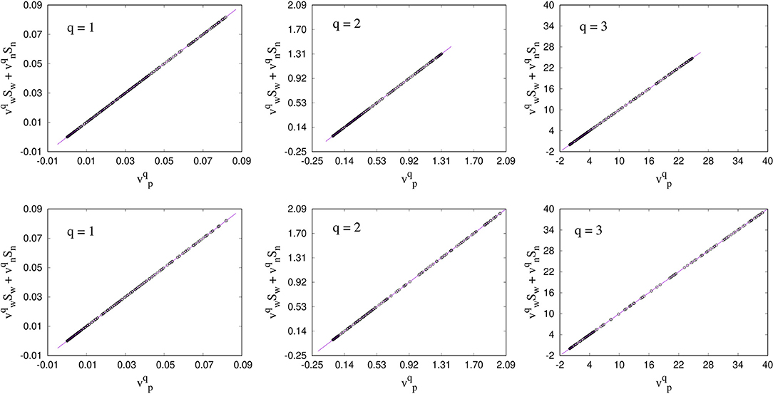
Figure 1. Verification of the relations (11), (45), and (59) between the steady-state seepage velocities vp, vw, and vn, and their higher moments for the 2D regular network. The top row represents the direct approach of measurements using Equations (79), (80), and (81). The bottom row corresponds to the velocities measured from the differential area distributions defined in Equations (58), (60), and (61). vp has a unit mm/s. Subsequently, for q = 2 and 3, the units for will be mm2/s and mm3/s, respectively.
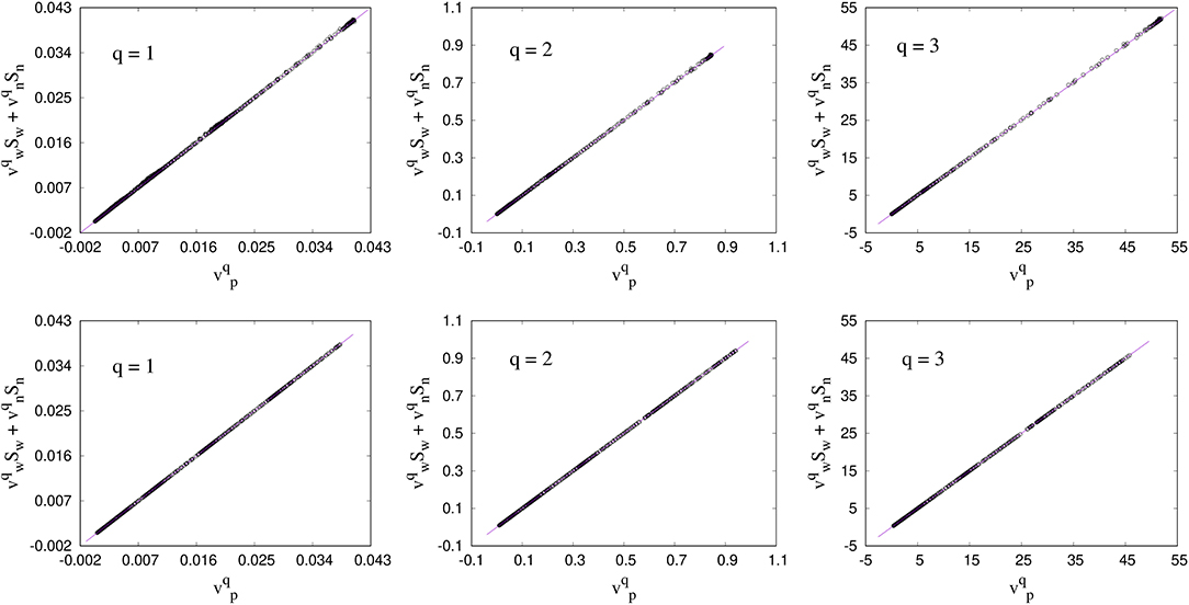
Figure 2. Verification of the relations (11), (45), and (59) between the steady-state seepage velocities vp, vw, and vn, and their higher moments for the 3D Berea network. The direct approach of measurements using Equations (82)–(84) are presented in the top row. The measurements using the differential area distributions defined in Equations (58), (60), and (61) are presented in the bottom row. vp has a unit mm/s. Subsequently, for q = 2 and 3, the units for will be mm2/s and mm3/s, respectively.
Next we measure the fluctuations in the seepage velocities which obey Equation (74). Numerically, , , and are calculated from the knowledge of the 1st and 2nd moments by,
In Figure 3, we plot these fluctuations for the two networks to compare with Equation (74) and good agreements is observed. There are some deviations in the results for the Berea network, since the results in 3D is based on only one network configuration whereas the results for 2D are averaged over 10 different configurations.
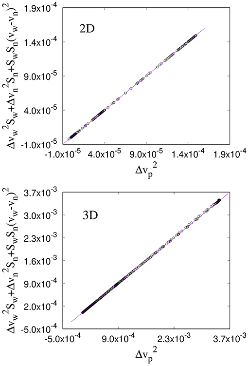
Figure 3. Numerical verification of Equation (74) between the fluctuations in the seepage velocities. has a unit mm2/s.
Finally, we verify the relations between seepage velocities and their higher moments while varying the fluid saturation as given by the Equations (29), (30), and (62). For this, we first calculated the co-moving velocity (vm) and its higher moments from Equations (29) and (30) where we used the values of the seepage velocities measured with the direct approach. This is shown in the top rows of Figures 4, 5 for 2D and 3D, respectively, which show good agreements with Equations (29) and (30). We then compare these values of with the measurements from the differential transversal areas using Equation (46). For this, we first constructed the histogram for the differential pore area am corresponding to the co-moving velocity from Equation (47) where we have used the variations of ap, aw, and an with the saturation Sw. For this purpose, we have considered 21 different values of saturations within 0 and 1 with an interval of 0.05. We then integrate am from −∞ to ∞, weighted by the velocity and normalized by the total pore area to obtain the desired co-moving velocity with Equation (46). These results are plotted in the bottom row of Figures 4, 5 where they are compared with the results from direct measurements. The data points roughly follow the diagonal straight line showing satisfactory agreement with the theoretical formulations. However, we observe deviations in the results that is higher compared to the direct measurements. We believe this is due to the numerical errors that added up from several steps in the calculation such as the binning techniques while measuring the distributions, taking the derivatives and calculating the integrals. Moreover, the fluctuations for 3D are much higher compared to 2D, which is due to the lack of averaging over different samples as we have already mentioned earlier.
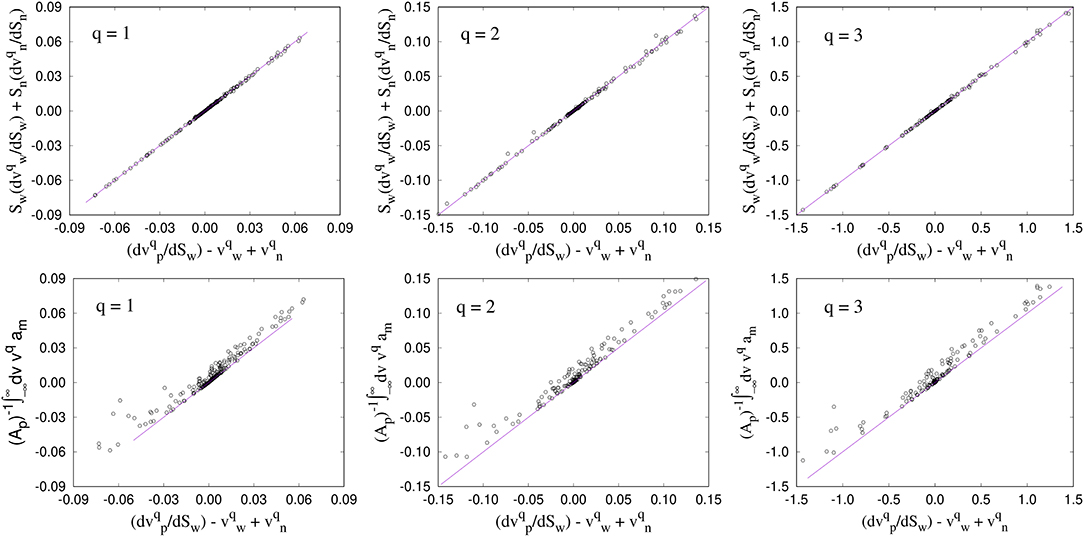
Figure 4. Measurement of the co-moving velocity (vm) and its higher moments for the 2D network. The top row corresponds to the calculations using Equations (29) and (30) with the direct measurements. The bottom row shows the measurements of using the differential area distributions with Equation (46) and compared with the direct measurements where higher fluctuations are observed. vm has a unit mm/s. Subsequently, for q = 2 and 3, the units for will be mm2/s and mm3/s, respectively.
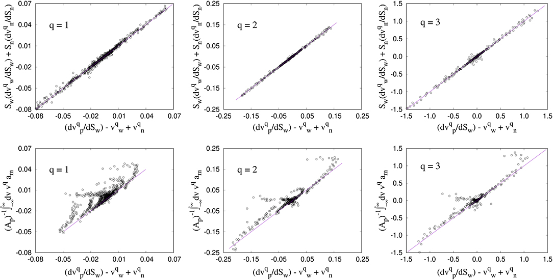
Figure 5. Measurements of for the 3D Berea network where the top row corresponds to the direct measurements using Equations (29) and (30), and the bottom row corresponds to the measurement from the differential area distributions using Equation (46). Here, larger fluctuations in the results calculated with the differential pore area are observed compared to the 2D network. vm has a unit mm/s. Subsequently, for q = 2 and 3, the units for will be mm2/s and mm3/s, respectively.
7. Summary
The aim of this paper is to provide the link between the pseudo-thermodynamic theory at the continuum level developed in Hansen et al. [21] (see section 3) and the velocities occurring at the pore level during immiscible two-phase flow in porous media. This link is provided by defining the differential transversal pore areas defined in section 4, which essentially correspond to the statistical distributions of velocities at the pore level. The central quantities are the velocity differential transversal pore area ap, the wetting fluid differential velocity transversal pore area aw, the non-wetting fluid velocity differential transversal pore area an, and the co-moving velocity differential transversal pore area am. We also consider the thermodynamic velocity differential transversal pore areas âw and ân. The relations found by Hansen et al.[21] for the average seepage velocities, the co-moving velocity and the thermodynamic velocities are generalized to the differential transversal areas here. In the following section 5, the relations are generalized to higher moments of the velocity distributions.
The theoretical derivations are then in section 6 validated by numerical simulations. We used dynamic pore-network modeling where an interface-tracking model is used to simulate steady-state two-phase flow. We used both regular pore networks and an irregular pore network reconstructed from a Berea sandstone for our simulations. By measuring the seepage velocities from the differential area distributions and comparing them with the direct measurements, we validated the essential predictions from the earlier theoretical sections.
Both Hansen et al.[21] and the present paper are to be seen as installments toward a theory for immiscible flow in porous media at the continuum scale. The structure of this theory reflects that found in thermodynamics: A set of general relations between the macroscopic variables based on energy conservation (i.e., the Gibbs relation) and Euler homogeneity. These general equations then have to be complemented by an equation of state which introduces the specifics of the system at hand. In the immiscible two-phase flow theory we are presenting here, Euler homogeneity and mass conservation provide the general equations that transcend the specifics of the porous medium. These general equations then have to be complemented by the constitutive equations for vp and vm, which provide the specifics of the porous medium.
The resulting set of equations may then be solved for structured porous media where the structure are associated with length scales larger than that set by the REV. This is e.g., seen in the explicit appearance of the porosity ϕ in Equations (34)–(36).
An open question, though, is what happens when there is non-trivial structure in the porous medium all the way from the pore scale to the continuum scale, see [37] and [38]—or when the saturation of the system is at a critical value, see [36]. The fundamental Euler scaling assumption (12) would then need to be modified, and with it, all the ensuing equations.
Data Availability Statement
The datasets generated for this study are available on request to the corresponding author.
Author Contributions
SR did the numerical simulations and analysis. SS developed the codes and performed the 3D simulations. AH developed the theory.
Funding
SS was supported by the National Natural Science Foundation of China under grant number 11750110430. This work was partly supported by the Research Council of Norway through its Center of Excellence funding scheme, project number 262644.
Conflict of Interest
The authors declare that the research was conducted in the absence of any commercial or financial relationships that could be construed as a potential conflict of interest.
Acknowledgments
The authors thank Carl Fredrik Berg, M. Aa. Gjennestad, Knut Jørgen Måløy, Per Arne Slotte, Ole Torsæter, Morten Vassvik, and Mathias Winkler for interesting discussions. AH thanks the Beijing Computational Science Research Center CSRC for the hospitality and financial support.
References
3. Wyckoff RD, Botset HG. The flow of gas-liquid mixtures through unconsolidated sands. Physics. (1936) 7:325–45. doi: 10.1063/1.1745402
5. Hassanizadeh SM, Gray WG. Mechanics and thermodynamics of multiphase flow in porous media including interphase boundaries. Adv Water Res. (1990) 13:169–86.
6. Hassanizadeh SM, Gray WG. Towards an improved description of the physics of two-phase flow. Adv Water Res. (1993) 16:53–67.
7. Hassanizadeh SM, Gray WG. Thermodynamic basis of capillary pressure in porous media. Water Resour Res. (1993) 29:3389–405.
8. Niessner J, Berg S, Hassanizadeh SM. Comparison of two-phase Darcy's law with a thermodynamically consistent approach. Transp Por Med. (2011) 88:133–48. doi: 10.1007/s11242-011-9730-0
9. Gray WG, Miller CT. Introduction to the Thermodynamically Constrained Averaging Theory for Porous Medium Systems. Berlin: Springer Verlag (2014).
10. Kjelstrup S, Bedeaux D, Hansen A, Hafskjold B, Galteland O. Non-isothermal transport of multi-phase fluids in porous media. The entropy production. Front Phys. (2018) 6:126. doi: 10.3389/fphy.2018.00126
11. Kjelstrup S, Bedeaux D, Hansen A, Hafskjold B, Galteland O. Non-isothermal transport of multi-phase fluids in porous media. Constitutive equations. Front Phys. (2019) 6:150. doi: 10.3389/fphy.2018.00150
12. Hilfer R, Besserer H. Macroscopic two-phase flow in porous media. Phys B. (2000) 279:125–9. doi: 10.1016/S0921-4526(99)00694-8
13. Hilfer R. Capillary pressure, hysteresis and residual saturation in porous media. Phys A. (2006) 359:119–28. doi: 10.1016/j.physa.2005.05.086
14. Hilfer R. Macroscopic capillarity and hysteresis for flow in porous media. Phys Rev E. (2006) 73:016307. doi: 10.1103/PhysRevE.73.016307
15. Hilfer R. Macroscopic capillarity without a constitutive capillary pressure function. Phys A. (2006) 371:209–25. doi: 10.1016/j.physa.2006.04.051
16. Hilfer R, Döster F. Percolation as a basic concept for capillarity. Transp Por Med. (2010) 82:507–19. doi: 10.1007/s11242-009-9395-0
17. Döster F, Hönig O, Hilfer R. Horizontal flow and capillarity-driven redistribution in porous media. Phys Rev E. (2012) 86:016317. doi: 10.1103/PhysRevE.86.016317
18. Valavanides MS, Constantinides GN, Payatakes AC. Mechanistic model of steady-state two-phase flow in porous media based on Ganglion dynamics. Transp Porous Media. (1998) 30:267–99. doi: 10.1023/A:1006558121674
19. Valavanides MS. Steady-state two-phase flow in porous media: review of progress in the development of the DeProF theory bridging pore-to statistical thermodynamics-scales. Oil Gas Sci Technol. (2012) 67:787–804. doi: 10.2516/ogst/2012056
20. Valavanides MS. Review of steady-state two-phase flow in porous media: independent variables, universal energy efficiency map, critical flow conditions, effective characterization of flow and pore network. Transp Porous Media. (2018) 123:45–99. doi: 10.1007/s11242-018-1026-1
21. Hansen A, Sinha S, Bedeaux D, Kjelstrup S, Gjennestad MA, Vassvik M. Relations between seepage velocities in immiscible, incompressible two-phase flow in porous media. Transp Porous Media. (2018) 125:565–87. doi: 10.1007/s11242-018-1139-6
23. Buckley SE, Leverett MC. Mechanism of fluid displacements in sands. Trans AIME. (1942) 146:107–17.
24. Joekar-Niasar V, Hassanizadeh SM. Analysis of fundamentals of two-phase flow in porous media using dynamic pore-network models: a review. Crit Rev Environ Sci Technol. (2012) 42: 1895–76. doi: 10.1080/10643389.2011.574101
25. Aker E, Måløy KJ, Hansen A, Batrouni GG. A two-dimensional network simulator for two-phase flow in porous media. Transp Porous Media. (1998) 32:163–86. doi: 10.1023/A:1006510106194
26. Gjennestad MA, Vassvik M, Kjelstrup S, Hansen A. Stable and efficient time integration of a dynamic pore network model for two-phase flow in porous media. Front Phys. (2018) 6:56. doi: 10.3389/fphy.2018.00056
27. Gjennestad MA, Winkler M, Hansen A. Pore network modeling of the effects of viscosity ratio and pressure gradient on steady-state incompressible two-phase flow in porous media. arXiv:1911.07490 (2019).
28. Sinha S, Gjennestad MA, Vassvik M, Hansen A. A dynamic network simulator for immiscible two-phase flow in porous media. arXiv:1907.12842 (2019).
29. Tallakstad KT, Knudsen HA, Ramstad T, Løvoll G, Måløy KJ, Toussaint R, et al. Steady-state two-phase flow in porous media: statistics and transport properties. Phys Rev Lett. (2009) 102:074502. doi: 10.1103/PhysRevLett.102.074502
30. Tallakstad KT, Løvoll G, Knudsen HA, Ramstad T, Flekkøy EG, Måløy KJ. Steady-state simultaneous two-phase flow in porous media: an experimental study. Phys Rev E. (2009) 80:036308. doi: 10.1103/PhysRevE.80.036308
31. Aursjø O, Erpelding M, Tallakstad KT, Flekkøy EG, Hansen A, Måløy KJ. Film flow dominated simultaneous flow of two viscous incompressible fluids through a porous medium. Front Phys. (2014) 2:63. doi: 10.3389/fphy.2014.00063
32. Savani I, Bedeaux D, Kjelstrup S, Sinha S, Vassvik M, Hansen A. Ensemble distribution for immiscible two-phase flow in porous media. Phys Rev E. (2017) 95:023116. doi: 10.1103/PhysRevE.95.023116
33. Washburn EW. The dynamics of capillary flow. Phys Rev. (1921) 17:273. doi: 10.1103/PhysRev.17.273
34. Sinha S, Hansen A, Bedeaux D, Kjelstrup S. Effective rheology of bubbles moving in a capillary tube. Phys Rev E.(2013) 87:025001. doi: 10.1103/PhysRevE.87.025001
35. Batrouni GG, Hansen A. Fourier acceleration of iterative processes in disordered systems. J Stat Phys. (1988) 52:747–73. doi: 10.1007/BF01019728
36. Ramstad T, Hansen A, Øren PE. Flux-dependent percolation transition in immiscible two-phase flow in porous media. Phys Rev E. (2009) 79:036310. doi: 10.1103/PhysRevE.79.036310
37. Parteli EJR, da Silva LR, Andrade JS Jr. Self-organized percolation in multi-layered structures. J Stat Mech. (2010) 2010:P03026. doi: 10.1088/1742-5468/2010/03/P03026
Keywords: porous media, thermodynamic relations, seepage velocity, steady state flow, two phase flow
Citation: Roy S, Sinha S and Hansen A (2020) Flow-Area Relations in Immiscible Two-Phase Flow in Porous Media. Front. Phys. 8:4. doi: 10.3389/fphy.2020.00004
Received: 27 November 2019; Accepted: 06 January 2020;
Published: 24 January 2020.
Edited by:
Daniel Bonamy, Commissariat à l'Energie Atomique et aux Energies Alternatives (CEA), FranceReviewed by:
Wenzheng Yue, China University of Petroleum, ChinaEric Josef Ribeiro Parteli, University of Cologne, Germany
Copyright © 2020 Roy, Sinha and Hansen. This is an open-access article distributed under the terms of the Creative Commons Attribution License (CC BY). The use, distribution or reproduction in other forums is permitted, provided the original author(s) and the copyright owner(s) are credited and that the original publication in this journal is cited, in accordance with accepted academic practice. No use, distribution or reproduction is permitted which does not comply with these terms.
*Correspondence: Subhadeep Roy, c3ViaGFkZWVwcm95MDMmI3gwMDA0MDtnbWFpbC5jb20=