 Eirik G. Flekkøy
 Marcel Moura
 Knut Jørgen Måløy
- PoreLab, The Njord Centre, Department of Physics, University of Oslo, Oslo, Norway
A chain which is made to flow from a container, forms a striking arch that rises well above the container top. This phenomenon is caused by the well known Mould effect and is explained by a supply of momentum from the container, causing an upwards kick. Here we introduce a theory that allows for dynamic fluctuations of the chain and compare with corresponding simulations and experiments. The predictions for the chain velocity and fountain height agree well with experiments. We also explore the underlying mechanism for this momentum transfer for different chain models and find that it depends subtly on the nature of the chain as well as on the container.
1. Introduction
The dynamics of ropes and chains have attracted scientific attention for centuries. They are found in biological systems, many different technologies, as well as in everyday life. Examples include our tenants, the DNA molecule, the tail of a cat, the line of a fly-caster, a whip, or the chain of a falling anchor. Hanging chains were studied by Galileo in the 1600's [1] and later these were shown to be catenaries by Huygens, Leibniz and John Bernoulli. The equations governing hanging and moving chains have been around for almost 400 years [1–3]. This fact, however, does not rule out the possibility that even the simplest systems may still exhibit surprising behavior [4–6].
When the end of a chain is dropped from a pile contained at some height above the floor, gravity will set it in motion, and eventually the whole chain will have flowed over the edge of the container. As this happens the chain rises far above the rim of the container. The first to communicate this striking effect was Mould [7] in a video that has caused more than 3 million views on YouTube. A chain that forms a rising, self-supporting arch which extends a significant height above its container is illustrated in the experiment of Figure 1.
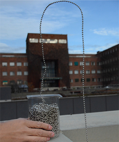
Figure 1. The flying chain resulting from a 5 m drop of the chain, photographed outside the physics building at the University of Oslo.
An analysis of the process was first carried out by Biggins [4] and Biggins and Warner [5]who demonstrated that the formation of a fountain depends on the existence of an upwards acting force that pushes the chain upwards and out of the container. This force has also been taken as the underlying mechanism for the fountain by other authors [8, 9].
In a recent paper Flekkøy et al. [10] we showed how simulations of a bead chain with realistic flexibility moving over a smooth and flat container bottom fail to produce a chain fountain. Only when an upwards acting force from a bumpy underlying packing is included, do the simulations produce a fountain, and this fountain survives when the rigidity of the links is removed in favor of a completely flexible bead chain. The difference between these two chains is the existence of a maximum bending angle between the links that connect the beads.
In this follow-up article, we proceed with a closer quantitative comparison between theory, simulations and experiments where the parameter space of the simulations is explored in some detail. Part of this exploration is a study of an experiment that may serve to distinguish between the different mechanisms that are responsible for the container force. This experiment measures the fountain height as a function of container width, and it is shown that different chain structures cause different dependencies between these quantities.
Even though strong spatial fluctuations are clearly visible in experiments, theoretical treatments of the chain generally assume a time-independent trajectory, that is, a steady state. In the present paper we develop a theory that goes beyond that simplification by allowing fluctuations, assuming only a statistical steady state where quantities such as momentum, are assumed steady only when averaged over sufficiently long times, or when ensemble averages are taken. We compare the predictions of the theory with measurements of the chain velocities. This is an interesting quantity in this context because it is sensitive to fluctuations around the steady state that is often assumed when analysing the chain dynamics. We find that the inclusion of dynamical fluctuations indeed improves the agreement with such measurements.
2. Momentum Conservation for a Dynamic Chain
Descriptions of the momentum balance of the chain exists in several text books, such as that on chain dynamics and shape [11] and the necessary equations of motion have been worked out in great detail [12, 13], at least for the steady state situations. We shall, however, take a general hydrodynamic description [14] of the momentum balance as the starting point, using the concept of continuum fields for mass and momentum densities to arrive at the averaged conservation laws for the chain with its fluctuating geometry.
Our Eulerian formulation of the chain dynamics uses the lab-frame of reference, since then it is easy to express the mechanical steady states.
2.1. Governing Equations From Conservation Laws
We start with the hydrodynamic style of expressing mass conservation
where the mass density ρ = λ/A vanishes outside the chain of cross-section A, u is the local velocity of the chain. In Figure 2A a piece of the chain is illustrated. The key observation is that a chain in motion may define a statistical steady state in which the chain might fluctuate but where the mass inside a given volume does not change when averaged over some time interval. We will assume ergodicity and replace the time-average by an ensemble average. As is commonly the case in statistical mechanics, such averages are simpler to deal with as they commute with both time-differentiation and volume averaging. Using that fact we may average and integrate (Equation 1) to get i.e.,
where the brackets denote an ensemble average. Equation (1) then gives
Integrating this equation over a suitable volumes containing piece of the chain we may apply Gauss' theorem.
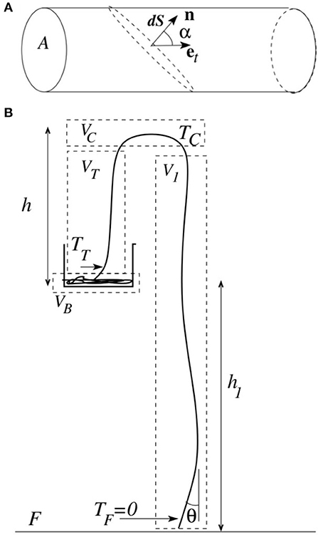
Figure 2. (A) The cross-section of a homogeneous chain. (B) The lengths defining the average chain configuration as well as the integration volumes and local tensions. The tensions are measured where the chain intersects the integration volumes. The floor at z = 0 is indicated by the horizontal line in the bottom of the figure.
Figure 2B illustrates such integration volumes. However, care must be taken to include only those areas of intersection where the ρ and u-fields are nonzero. When the surface elements are at an angle to the chain tangent et, integration gives the effective replacement dS → A/|n·et|. These are the areas of intersections with the chain. Carrying out such an integration of Equation (3) yields
where the unit vectors are defined in Figure 2A and i labels the intersections.
Just like in the case of the mass we may assume that the momentum inside a given volume remains constant in the sense that the average ∂t〈ρu〉 = 0. Now, the hydrodynamic equation for momentum conservation is
where f is an external force, g gravity and the stress tensor for a flexible chain with tension T, is
The steady state assumption leaves us with the averaged force-balance condition
Carrying out a volume integration of Equation (7) yields
where we have used the fact that dS·et/n·et = dS, and introduced . Equation (8) is our basic expression for momentum conservation. It expresses the momentum flux as a sum of an advective term and a tension term, and the sum of these terms balances the external forces on the right hand side. Note that Equation (8) may only be used to determine the sum of the advective- and tension terms and cannot itself be used to separate these terms. Only when either the tension or the advection term is known independently may solutions for the other term be obtained. We take this to happen where the chain hits the floor, setting TF = 0 there.
When the chain shape is stationary, on the other hand, u = etu with a constant u, and there is no ambiguity. In this case, if we define our integrations volumes so that n ∥ et everywhere, Equation (8) reduces to
with u constant. If u = 0 = F this equation could be used to obtain the well known catenary solutions for hanging chains. This may be achieved by making L infinitesimal, L → δs, a length element along the chain, so that the equation takes the form
Taking the tangential and normal components of this equation allows the integration of both T and et along the chain. Once such a solution is found with a tension T0(s), it also gives the u ≠ 0 solution with the tension . That is, the shape does not change, only the tension.
2.2. Asymptotic Velocity
In the following we will work out the fountain height h and the asymptotic mean square velocity , which we shall take as the basis for comparison. For this purpose we apply Equation (8) to the integration volumes of Figure 2B We will take the volumes VC and VB to be small enough to neglect gravity and only in VB will f ≠ 0. Here, the chain will pick up an upwards force from the coiled chain over which it moves. The collisions associated with this movement, will cause a momentum input that we associate with f and when integrated over VB gives a force .
Taking the z-component of Equation (8), and assuming that for symmetry reasons T is the same on either side of VC we get1
where the subscript C signals that the value in the parenthesis is to be evaluated at the intersection with the boundary of VC, and the + sign corresponds to the intersection of the upwards moving chain where etz > 0. We have used that the unit normal n = −ez.
In Equation (11) both the etz-factors will contribute to increase 〈TC〉 since they are smaller than one. The first factor exists because the tension acts along a variable direction and the second because momentum is advected over an intersection surface that depends on α as is illustrated in Figure 2A.
Now, we may integrate over V1, which gives
where 〈L1〉 is the average chain length contained in V1. We will take the tension TF at the bottom of the volume to vanish.
It has been observed- at least for some types of chains- that the interaction between the falling chain and the floor may produce an added downwards force, causing freely falling chains to accelerate slightly faster than gravity [13]. However, for the sake of simplicity, we shall in the following neglect this interesting, but small effect and assume that TF = 0. Then the TF-term above vanishes, and the first and third terms cancel due to Equation (11). This leaves the velocity equation
This equation shows that the velocity is governed by the weight of the downwards moving part of the chain, λ〈L1〉g. This means that buckling of the chain, which will increase 〈L1〉, will increase the velocity with which it falls.
In order to simplify (Equation 13) we note that |etz| = cos Θ where Θ is the local chain-angle to the vertical. As the tension goes to zero toward the floor, it may be reasonable to assume a de-correlation between Θ and uz. Also, for small angles we may Taylor expand to get
with an error that enters only at 4. order in Θ. We may then write
This is the prediction that will be compared with the simulations and experiments.
2.3. Fountain Height
In order to get a prediction for h, we must integrate over VT and VB. For beads at rest in the container gravity is balanced by the force from below that keep them from falling. We therefore introduce
the net force on the beads in VB. This force is non-zero only for moving beads. Furthermore, the momentum advection is non-zero only at the top of the VB-surface, so the z-component of Equation (8) then takes the form
Doing the same for volume VT gives
where LT is the length of chain contained in VT. Here the first two terms on the left hand side cancels due to Equation (11) and the last two terms may be replaced by −〈ΔFz〉 due to Equation (19). This leaves the fountain equation
This shows that LT = 0 and thus h = 0 unless there is a vertical force from the container. However, an additional relation between LT and h is needed. We will show numerically that this relation is indeed linear, so that
In order to get a theoretical relationship between h and h1 we need a model for the force ΔFz. The simplest possible model for the container force relies on the notion that it is caused by collisions between the beads that are accelerated along the bottom, and the beads that are still stationary. Each impact will happen at a rate ∝u and contribute a momentum ∝u and thus on the average. Then, if we assume that , Equation (17) implies that
The last equality follows since, if h∝h + h1, then h ∝ h1. By postulating, or measuring, constants of proportionality between ΔF and , between 〈L1〉 and h1, and between 〈h〉 and 〈LT〉, it is straightforward- though not very enlightening- to produce the constant of proportionality between h and h1.
2.4. Biggins Equations for the Fountain Evolution
However, for the purpose quantifying the effect of fluctuations it is useful to compare the above theory with one that ignores them. It is therefore instructive to point to an elegant analytical formulation of the chain evolution, which is given by Biggins in Equations (11) and (12) in Biggins [4]. This theory disregards fluctuations but includes the evolution of the fountain. It uses a model where and the fitting parameter α = 0.12. With this value of α good agreement in terms of the predicted and measured values is observed. The theory implies that the only relevant time scale for the relaxation of h(t) is .
3. Experiments
We have performed experiments using a 50 m long chain of metallic beads having diameters of 4.5 mm. We believe this to be the same kind of chain used by Biggins [4] and other authors. We have noticed that the way the chain is stacked in the container is crucial in order to avoid entanglement. We start by piling up the chain at a given location by the wall in the container, and then, after the pile has grown large enough that its base is reaching the middle of the container, we move to the opposite side of the container and repeat the procedure. The third location is at the wall midway between the two first ones, and the fourth and final location opposite to the third one. After that, we move again to the first location and go on like this until the whole chain fits inside the container. Earlier a circular spiral packing was attempted but that turned out to lead to more clumping and knot-like structures which would always bring disturbances to the chain.
Images were acquired with three cameras operating on different modes. A high resolution Nikon D7200 DSLR camera is used to obtain images of the whole chain and is placed on a high tripod about 3 m away from the system. A Photron SA5 high speed camera was used to image the descending segment of the chain. The images were captured close to the ground at a framerate of 4000 fps. An additional set of high speed images was captured by a Nikon J4 camera at 1000 fps to capture the details of how the beads take off inside the container.
The Photron high speed images were used to measure the vertical speed component uz. This was done by tracking the motion of individual beads in the chain. Figure 3 shows an example of the action of the bead tracking algorithm. The bead marked with a filled green circle is tracked in the following frames and its position on each future frame is shown by an open red circle. The tracking happens for 50 frames during 12.5 ms. Notice that the motion of a single bead does not necessarily follow the path of the chain, i.e., there can be a component of the bead velocity perpendicular to the chain's tangent vector (as noted in the previous section, the vectors u and et are not necessarily parallel).
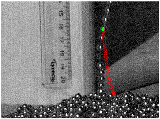
Figure 3. Example of bead tracking using a series of high speed images. The filled green circle corresponds to the current position of one particular bead being tracked and the red open circles correspond to later positions of the same bead. The tracking lasts for 50 frames here corresponding to a time span of 12.5 ms.
In order to determine how the momentum transfer takes place, we have performed an additional experiment where high speed footage inside the container was acquired, to image the chain take-off process. Typical images are shown in Figure 4, where we have colored a segment of beads to follow its motion. The chain extends horizontally over a significant part of the container, thus accumulating momentum over a series of collisions with the underlying chain as it is dragged along before taking off. We did not observe a frequent occurrence of large bending angles, but often a formation of a stationary spiral hitting the underlying packing at its bottom could be observed. In the time frames between the first and last images in the figure, we see that the chain was dragged by about 2 bead diameters in 7.5 ms. This observation corroborates the idea that the necessary momentum transfer happens more in the way of a bumpy take-off than by the kick-off mechanism, as previously noted in Flekkøy et al. [10].
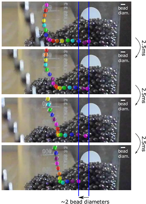
Figure 4. A time sequence of 7.5 ms using a 50 m chain of 4.5 mm beads. Individual chain beads are traced by different colors. Adapted from Flekkøy et al. [10] with permission from the authors.
4. Simulations
The simulations are based on a particle representation of the individual beads of the chain and integrate the equations of motion that derive from Newtons second law in 3 dimensions. The algorithm resembles that used by Vrbik [15] who studied the motion of a chain falling off the edge of a table. The chain is initially at rest and is hanging from the container to the table.
4.1. The Particle Forces
The beads in the chain are taken to interact through a harmonic potential with an equilibrium separation a0, i.e., if the separation between two neighboring particles is Δr = r1 − r2 then
Also, an interparticle dissipative force −βΔv, where Δv is the relative velocity between neighboring particles. This force dampens longitudinal fluctuations, which is certainly realistic. However, no corresponding angular friction is included, which means that transverse waves will tend to die out more slowly than in the experiments. The container is implemented both by conservative and dissipative forces: The side walls and top rim of the container are implemented by a conservative potential like that of Equation (24), but with a force that always pushes the particle away from the walls and top rim. At the bottom, however a horizontal dissipative force, or sliding friction, −βcv∥, where v∥ is the horizontal velocity component, is included. This force dampens the motion inside the container that would remain for a long while if there were only the inter-particle dissipation.
4.2. Geometric Boundaries
Since the beads have only nearest neighbor interactions, the interaction between a bead and the underlying chain packing cannot be done by bead interactions. In stead we introduce a rough container bottom. Attempting to make this roughness correspond to the packing we use the bottom height function
where x and y are the horizontal coordinates. The resulting bottom profile is illustrated in Figure 5A. The choice a = 0.25a0 comes close to mimicking the geometry of the chain itself.
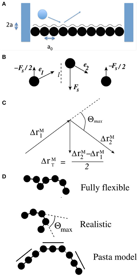
Figure 5. (A) Model of the bead packing in terms of a rough bottom. (B) The stiffness force is distributed so that the total force vanishes. (C) The transverse displacement vector when Θ = Θmax. (D) The various simulated chains with differing internal stiffness interactions. Adapted from Flekkøy et al. [10] with permission from the authors.
The floor, which is located at z = 0 is implemented by a adding a strong vertical damping in the form of another frictional force −βFvz. Newtons second law is then integrated using a Velocity Verlet scheme of 4'th order accuracy in time.
The distance b between the bead center and the bottom at which the interaction sets in, is normally equal to half the interbead distance, i.e., b = a0/2, but may also be taken to be smaller, thus simulating smaller beads. The interaction between the particles and the boundaries (side walls and rough bottom) are derived from a harmonic potential so that the interaction force is implemented as a repulsive spring force which is linear in the overlap length.
4.3. The Stiffness Force
The internal stiffness force is introduced to keep the chain from bending. It acts on the particle that is in the middle of a stiff 3-particle segment and in order to keep it an internal force, an equal and opposite counterforce is distributed on the two nearest neighbors. It is implemented by the following force
where k is the spring constant and e2, e1 the unit vectors pointing between the neighbors, as is illustrated in Figure 5B. This force is linear in departure from straightness, i.e., the length l <between the particle and the line joining the nearest neighbors on either side. Note that when k is sufficiently large that the action of the potential in Equation (24) has brought the particle separation to a0, the a0(e2−e1) ≈ r2 − r1. To obtain a piecewise rigid chain, Fs is applied to every third bead. By choosing k sufficiently large, a sequence of rigid rods composed of three beads each, is created.
It is possible to generalize this force in a way so that it only kicks in when the angle Θ between e2 and e1 exceeds a maximum value Θmax.
For this purpose we introduce the transverse displacement vector ΔrT which is the displacement of a particle from the line that connects its two nearest neighbors. This vector is illustrated in Figure 5C for the case when Θ = Θmax. We require that the restoring stiffness force be linear in the increase in ΔrT above the Θmax value, i.e.,
Now, this force acts along with the interaction forces that produce a particle separation near a0, so we may assume that these other forces have already caused such a separation, and we approximate Δri = a0ei. Assuming also that the new displacement vector , we may write
when Θ ≥ Θmax. Using the fact that the ei's are unit vectors with internal angles Θ and Θmax, the force then takes the form
This force is applied to every bead. If Θmax is zero this would result in a long rigid chain, so we choose it in stead to the measured value Θmax = 63 degrees. When Θmax is zero, and the force is applied to every third particle, the model of Equation (26) is reproduced.
As experiments with the piecewise rigid chain may be carried out using pieces of pasta, the corresponding model used in the simulations will henceforth be termed the pasta model. The different chain models are illustrated in Figure 5D.
Initially, the chain is packed in the container in straight segments that extend between points on the container wall. As the beads are added and meet the wall, a random new direction pointing into the container, is chosen.
5. Results and Discussion
In the following we explore the mechanisms producing the force ΔF (see Equation 18) by applying the simulations with different bottom roughnesses, chain models and container widths.
Figure 6A shows the result of a simulation using a = 0.25a0 and Θmax = 63°. The fountain must acquire its asymptotic height before 〈h〉 is recorded. Figure 6B shows a direct comparison between simulations and experiments. Figure 7 shows that indeed the relationship between LT and h is linear. The slope of 1.25 is a measure of the chain buckling and also the difference between a theory that includes fluctuations and one that does not.
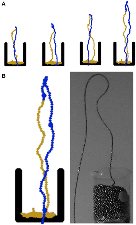
Figure 6. (A) A simulated time sequence of the fountain evolution shown at times t = 1.8, 2.0, 2.5, and 3.5 s. The beads are all of equal size and properties, the larger beads are only drawn in order to track the beads which are colored blue when they are outside the horizontal extent of the container and given a brass color when they are not. (B) Simulated and experimental fountain.
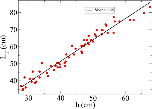
Figure 7. The length LT of the upwards moving part of the chain as a function of fountain height h as measured by simulations.
5.1. Fountain Height and How It Changes With Different Models
In order to check the effect of variations of the container bottom, we measured h as a function of the amplitude a that enters in Equation (25) (see Figure 8). It is seen that when a > 0.4 a0, there are only weak variations in h with a.
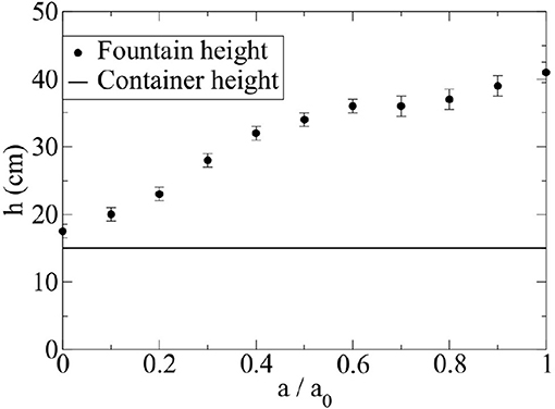
Figure 8. Fountain height h as a function of bottom roughness a when h1 = 4 m. The container height is the vertical extent of the container and thus a minimum value for h.
Observing that a bumpy packing, or container bottom, is crucial to produce a fountain both for the realistic and fully flexible chain, we may still inquire if there are any other chains that do not rely on the structure of the bottom. Indeed, Biggins [4] explored two additional chains, one that was composed of piecewise rigid segments, thus corresponding more closely to his theoretical model, and one with well separated beads, which could not support the kick-off effect. The results were that the first chain did produce a fountain, and the latter not.
However, doing the same in our simulations, using (i) a fully flexible separated bead chain having rigid segments of length 3 cm, and the bottom roughness a = 3 mm as before, and (ii) a piecewise rigid chain with a perfectly smooth container bottom, we observe a fountain in both cases. Figure 9 shows a time sequence using the flexible (Θmax = π) separated bead model with a rough bottom. Figure 10 shows a time sequence using the pasta model with a smooth bottom. Note that this is the only chain model that produces a fountain in the absence of bottom roughness. This observation is consistent with the experimental observations of Pantaleone [8] who sees an increase in h when a chain of balls was replaced by a similar chain of elongated rods.
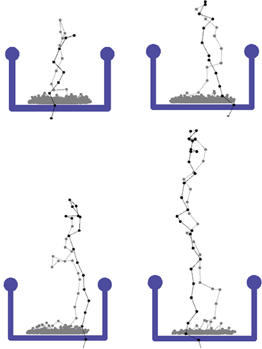
Figure 9. A simulated time sequence of the fountain evolution using the separated beads model.
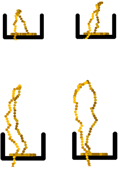
Figure 10. A simulated time sequence of the fountain evolution using the pasta model. The times are 0.5, 2.0, 2.5, and 3.0 s and h1 = 1.8 m.
In Figure 11 we collect the results of all the different chain models measuring h as a function of h1. They are carried out by simulating the different chain and container models. We have also included the original measurements of Biggins and Warner [5]. Our realistic simulations using a bottom roughness a = a0/4 agree well with these. We have truncated the measurements at h1 = 4 m as the chain lengths which have been applied, do not allow the system to reach a steady state above that container elevation. Andrew et al. [16] report a non-linear relationship between h and h1 using a chain of length 41.5 m and elevation heights up to 18 m. For such elevations one would need a chain more than 200 m long to reach the asymptotic h-value. So, in this case the non-linear relationship would appear to exist only between h1 and some transient value of h.
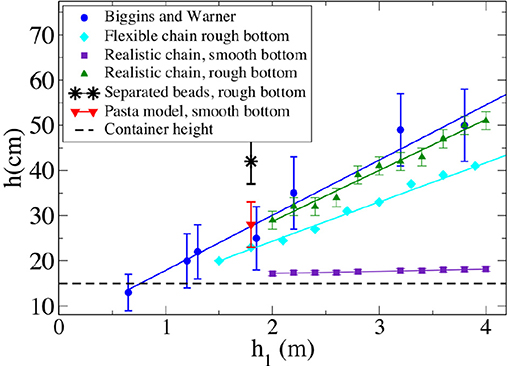
Figure 11. The fountain height as a function of elevation h1 for the different models. Reproduced from Flekkøy et al. [10] with permission from the authors.
5.2. Fountain Height and Container Width
It is seen that the combination of a realistic chain and a smooth bottom produces no fountain, thus ruling out the kick-off mechanism as a complete explanation for the phenomenon. The kick-off mechanism by itself only works to explain the chain fountain of the pasta model. However, it is seen that while both the realistic and flexible chains rely on a rough bottom to produce a fountain, the existence of a realistic rigidity enhances the fountain.
Is there a crucial experiment that may serve to distinguish between the different mechanisms? The fountain produced by the pasta-model on a smooth container bottom (a = 0) can only be explained by the kick-off mechanism, while the fountain of the flexible (Θmax = π) model can only be explained by the bumpy take-off mechanism. Figure 12 shows how h varies with the container width for these models. The container is kept at fixed proportions so that its height is equal to its width. It is seen that the pasta model and the flexible chain exhibit opposite trends with increasing w. The most realistic model, the realistic chain on a rough bottom, however has less of a pronounced trend, although it tends to behave more like the pasta model. The realistic chain on a smooth bottom, on the other hand, has no fountain as h ≈ w (the w = 5 cm point is also likely to be a result of chain-container rim interactions). Note that the pasta model too seems to lose its fountain as the container width is increased.
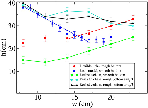
Figure 12. Fountain height as a function of container width w h1 = 2.5 m.
5.3. Velocity Measurements
The predictions for the velocity of the chain given by Equation (17) involves the mean square velocity
This is indeed what is measured in the simulations and experiments. A comparison between measurements and the prediction of Equation (17) is shown in Figure 13. First, it is clear that Equation (17) agrees well with the simulations using the realistic model of the chain and container, but not so well with the experiments.
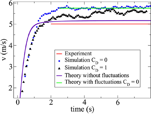
Figure 13. Velocities measured 20 cm above the floor. The red line shows the experimental average where uz is the vertical component of the velocity. The blue circles show simulation measurements taken at the same location but as a function of time. The indigo line shows a semi-analytic prediction derived from Equations (11) and (12) in Biggins [4], which is based on a fluctuation-less model. The green horizontal line shows the analytic prediction of Equation (17) and should be compared with the simulation of the velocity at the floor. The triangles show simulations with air-drag included.
This is most likely due to a combination of two factors: (1) lack of hydrodynamic drag from the air, and (2) lack of bending friction in the simulations. The hydrodynamic drag may be added to the simulations by including a force per bead where ρair is the mass density of the air, A is the cross-sectional area of a sphere, and CD is the drag coefficient of a bead, in the force calculations. For single sphere CD ≈ 0.5, but our spheres are equipped with pins connecting to their neighbors and also move together in a direction that is often not parallel to the chain itself. These factors may cause CD to increase, and we have tentatively set CD = 1. The result, which is shown in Figure 13, is seen to bring the simulations closer to the experiments, but not to a full agreement. The other factor, the lack of bending friction, is likely to cause more chain buckling, and hence a larger L1-value than in the experiments. This is consistent with visual observations of the real and simulated chains, see Figure 6B. From the experiments we estimated that the increase in length of the downward section of the chain due to buckling is only of 1.5%, which is much less than the order 25% buckling that we see in the simulations. Since larger fluctuations should, according to our theory, lead to a larger chain velocity, it makes perfect sense that the experimental velocity falls below the one of theory/simulations.
Mass conservation then implies that . Also, simulations lack any dissipation associated with beads colliding with the rim of the container and therefore produces a slightly larger velocity than the experiments.
The analytic, fluctuation free prediction of Biggins is seen to lie below the present simulations, at least asymptotically. Biggins asymptotic v- value does not depend on α, and would in fact agree with Equation (17) if the replacement 〈L1〉 〈cos Θ〉 → h + h1 was done. This means that the disagreement is most likely due to the added mass in the downwards moving chain due to the fluctuations.
It should be noted that the prediction of Equation (17) for the average velocity 〈uz〉 itself reflects both the geometric effect of the fluctuating chain and the effect of velocity fluctuations δuz around the average as . Naturally, in the stationary limit these effects both go away.
There is a fine point linked to the measurement of uz and the fact that our continuum theory of Equation (8) is compared to a discrete particle model. Indeed, the velocity varies discontinuously from particle to particle, and only when their velocities are averaged into a group does it make sense to represent them by a differentiable field as we do. The velocities, and by implication the cos Θ-values, shown in Figure 13 are averaged over groups of 10 particles. Reassuringly, the result changed by less than 1% when the group was enlarged to 20 particles.
Figure 14 shows measurements that follow a single particle as it approaches the location where it stops. The vertical component of velocity is recorded, and the distance to the floor packing is exactly the distance to the future stopping location. The rightmost vertical line shows where forces from the floor are observed to slow the chain down. The leftmost line is drawn at a distance a0, above which there can be no direct interaction between the bead and the underlying packing. The fact that the beads start slowing down above the distance a0 means that there must be an upwards acting force that is transmitted through the chain to the particle when it is located between the two lines. This can be more clearly seen by visually comparing a group of three consecutive beads close to the packing (green square in Figure 14) to a similar group of beads a bit further up (purple square). We see that the beads close to the packing seem to be compressed together, indicating the presence of an upwards force from the floor.
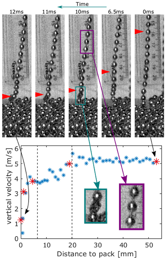
Figure 14. Velocities measured at different heights above the floor. The graph shows how the upwards forces, coming from the interaction with the floor, slow down the beads. The rectangular frames illustrate how a group of three beads is compressed as it hits the packing. The rightmost vertical line shows where forces from the floor are observed to slow the chain down. The leftmost line denotes the distance a0, above which there can be no direct interaction with the underlying packing.
This observation runs contrary to the observation by Grewal et al. [13] who found that the interaction with the floor might cause a falling speed slightly faster than free fall.
6. Conclusions
In summary, we have developed a theory of the flying chain motion that includes fluctuations, and we have proceeded to demonstrate, mainly via simulations, that these fluctuations play a quantitative role that is necessary for the theory to agree with measurements. The simplest observation of this is the fact that chain buckling creates an increased effective mass in the chain by about 25%.
The existence of a fountain relies entirely on the upwards acting force from the container on the chain. But the mechanisms acting to produce this force varies depending on the construction of the chain. While a chain made of rigid segments may create a fountain even when it takes off from a smooth container bottom, this is not the case for a chain with flexible links between spherical beads. In this case the required momentum must be picked up from the container via collisions with beads in it or a rough container bottom. Yet, the introduction of a maximum bending angle between links in the chain, will enhance the effect of these collisions.
We have studied an experiment that may serve to distinguish the mechanisms at play, that is, the measurement of fountain height vs. container width. While the rigid segment tend to reduce its fountain height with increasing width, the opposite is true for the flexible chain without a maximum bending angle between links in the chain.
Data Availability Statement
The datasets generated for this study are available on request to the corresponding author.
Author Contributions
EF did the theory and simulations as well as the main part of the writing. MM did the experiments as well as the written description of those, while KM having developed the labs that made the experiments possible supervised these. All authors contributed to the discussions defining the work.
Conflict of Interest
The authors declare that the research was conducted in the absence of any commercial or financial relationships that could be construed as a potential conflict of interest.
Acknowledgments
We wish to thank Ellen Karoline Henriksen and Carl Anghell who first introduced us to the flying chain, Dragos-Victor Anghel for his valuable theoretical input and Frédéric Lindboe for his practical tips on how to pack the beads. We also thank the Research Council of Norway through its Centres of Excellence funding scheme, project number 262644.
Footnotes
1. ^This result may also be proven by integrating over only half the VC volume and assuming 〈uzux〉 = 0 on the vertical surface of this volume.
References
1. Drake S. Two New Sciences. Madison, WI: University of Wisconsin Press (1974). (Original work by Galilei G. published in 1638).
4. Biggins JS. Growth and shape of a chain fountain. Europhys Lett. (2014) 106:44001. doi: 10.1209/0295-5075/106/44001
5. Biggins JS, Warner M. Understanding the chain fountain. Proc R Soc A. (2014) 470:20130689. doi: 10.1098/rspa.2013.0689
6. Hanna JA, Santangelo CD. Slack dynamics on an unfurling string. Phys Rev Lett. (2012) 109:134301. doi: 10.1103/PhysRevLett.109.134301
7. Mould S. Web Page (2013). Available online at: http://stevemould.com/siphoning-beads/
8. Pantaleone J. A quantitative analysis of the chain fountain. Am J Phys. (2017) 85:414–21. doi: 10.1119/1.4980071
9. Pfeiffer F, Mayet J. Stationary dynamics of a chain fountain. Arch Appl Mech. (2017) 87:1411–26. doi: 10.1007/s00419-017-1260-y
10. Flekkøy EG, Moura M, Måløy KJ. Mechanisms of the flying chain fountain. Front Phys. (2018) 6:84. doi: 10.3389/fphy.2018.00084
11. Routhe EJ. An Elementary Treatise on the Dynamics of a System of Rigid Bodies: With Numerous Examples. London: MacMillan (1860).
13. Grewal A, Johnson P, Ruina A. A chain that speeds up, rather than slows, due to collisions: how compression can cause tension. Amer J Phys. (2011) 79:723. doi: 10.1119/1.3583481
Keywords: flying chain, continuum mechanics, ropes and cables, strings, outreach
Citation: Flekkøy EG, Moura M and Måløy KJ (2019) Dynamics of the Fluctuating Flying Chain. Front. Phys. 7:187. doi: 10.3389/fphy.2019.00187
Received: 20 May 2019; Accepted: 29 October 2019;
Published: 19 November 2019.
Edited by:
Miguel Rubi, University of Barcelona, SpainReviewed by:
Alexandre De Castro, Brazilian Agricultural Research Corporation (EMBRAPA), BrazilRodolfo Morales, National Polytechnic Institute, Mexico
Copyright © 2019 Flekkøy, Moura and Måløy. This is an open-access article distributed under the terms of the Creative Commons Attribution License (CC BY). The use, distribution or reproduction in other forums is permitted, provided the original author(s) and the copyright owner(s) are credited and that the original publication in this journal is cited, in accordance with accepted academic practice. No use, distribution or reproduction is permitted which does not comply with these terms.
*Correspondence: Marcel Moura, bWFyY2VsbW91cmFAeWFob28uY29tLmJy