 Juan Mateos Guilarte
 Jose M. Munoz-Castaneda
 Irina Pirozhenko
 Lucia Santamaría-Sanz
95% of researchers rate our articles as excellent or good
Learn more about the work of our research integrity team to safeguard the quality of each article we publish.
Find out more
ORIGINAL RESEARCH article
Front. Phys. , 16 August 2019
Sec. Statistical and Computational Physics
Volume 7 - 2019 | https://doi.org/10.3389/fphy.2019.00109
This article is part of the Research Topic Contact Interactions in Quantum Mechanics: Theory, Mathematical Aspects and Applications View all 16 articles
We study the spectrum of the 1D Dirac Hamiltonian encompassing the bound and scattering states of a fermion distorted by a static background built from δ-function potentials. After introducing the most general Dirac-δ potential for the Dirac equation we distinguish between “mass-spike” and “electrostatic” δ-potentials. Differences in the spectra arising depending on the type of δ-potential are studied in deep detail.
The Dirac equation with various relativistic potentials mimicking string-like or vortex-like backgrounds has a long history. The best known example is the Aharonov-Bohm [1] interaction of charged fermions with a field of an infinitesimally thin solenoid. The scattering of fermions on magnetic 'tHooft-Polyakov monopoles and on Abrikosov-Nielsen-Olesen strings with consequent fractional fermion numbers and fermion number non-conservation was a hot topic in the late 70s and early 80s [2, 3]. The cosmic strings predicted by grand unified theories also appeared to interact with fermions (matter) via the Aharonov-Bohm mechanism [4]. The non-relativistic limit of the scattering problem for spin-one-half particles in the Aharonov-Bohm potential in (1+2) conical space was examined in [5, 6].
It was observed that in the case of a point magnetic vortex (Aharonov-Bohm interaction) one can either with gauge transformation reduce the problem to a Laplace equation with delta-potential or to a free Dirac equation with a special angular boundary condition [7]. A radial boundary condition specifies the self-adjoint extension. From the operator theory viewpoint the Dirac operator with relativistic point interaction (δ-function potentials) and its self-adjoint extensions were considered in [8, 9]. In the last years the low-dimensional problems of this kind were investigated topologically with the Levinson theorem, which proved to be closely related to an index theorem [10].
A renewed interest to Dirac equation with singular potentials was inspired by the appearance of the new 2D materials. Graphene in the field of a Aharonov-Bohm solenoid perpendicular to its plane was considered in [11]. The induced current and induced charge density were calculated. Another example is a magnetic Kronig-Penney model for Dirac electrons in single-layer graphene developed in [12]. The model is a series of very high and very narrow magnetic δ-function barriers alternating in sign.
In this paper we describe the distortion caused by impurities in the free propagation of fermionic fields in the 1 + 1-dimensional Minkowski spacetime by means of Dirac δ-point interactions. We elaborate on and develop further previous work on this subject in References [13, 14]. The matching conditions appropriated to define the δ-potential inserted in a Dirac Hamiltonian restricted to a line were proposed some time ago in References [15, 16].
Our aim is to generalize the study carried out in References [17–19] to fermionic fields so that we can use the results in effective QFT models of 2D materials.
Throughout the paper we shall use natural units where ℏ = c = 1 (henceforth, L = T = M−1). In addition we will fix the Minkowski spacetime metric tensor to be: ημν ≡ diag(+, −). Having done these choices, the Hamiltonian form of the Dirac equation, governing the dynamics of a free fermionic particle of mass m moving on a line, reads
or, in covariant form:
For the fermionic anti-particle the dynamics is governed by the conjugate Dirac Hamiltonian
or, in covariant form
Here, the matrices close the Clifford algebra of ℝ1, 1 that can be minimally represented by “pseudo-Hermitian”two-by-two matrices: γμ† = γ0γμγ0. Explicitly,
We shall need also the 1+1-dimensional analogue of the γ5 matrix, denoted throughout this paper as γ2:
The free Dirac Hamiltonians appearing in the formulas (1)–(2) demand thus the definition of the α and β Dirac matrices:
In order to perform explicit calculations we shall stick to the following choice of γ-matrices:
where σ1, σ2, σ3 are the Pauli matrices:
Our choice of gamma matrices enables us to identify the three discrete transformations acting on the Dirac spinors:
1. Parity transformation , where p = 0, 1, is the intrinsic parity of the particle
2. Time-reversal transformation .
3. Charge conjugation transformation .
Parity and time-reversal are symmetries of the free Dirac Hamiltoninan (1) and its conjugate (2). Charge conjugation, however, transforms the free Dirac Hamiltonian into its conjugate and viceversa. This property is the secret behind the common wisdom in Fermi field theory where negative energy fermions are traded by positive energy antifermions. More precisely: both and have a Dirac sea of negative energy states. The idea is to form a complete set of spinors from the positive energy states of , fermions, and the positive energy eigen spinors of , anti-fermions. In this spirit one checks that the solutions for the conjugate Dirac equation are related to the solutions of the Dirac equation by the charge conjugation transformation. Given the spectral problems
the eigenspinors are related through charge conjugation: . Equivalently, one finds that: .
Consider next a bunch of relativistic Fermi particle propagating in (1+1)D Minkowski spacetime under the influence of a external time-independent classical background. The most general Dirac Hamiltonian describing this situation reads:
The external potential comprises four types (see [14]):
In Ref. [14], it is shown that:
• It is possible to assume V1(x) = 0 without loss of generality since it can be absorbed by a gauge transformation.
• It is convenient to choose V3(x) = 0 to avoid interactions of the type which are only consistent if V3 is purely imaginary.
Hence, we shall focus our attention on background potentials of the form
leading to the following Dirac spectral problem
In formula (8) the ξ(x) potential clearly appears as an electrostatic potential, whereas the potential energy M(x) shows itself as a position dependent mass. Note that this last potential can be reinterpreted as an interaction of the Dirac field with a classical scalar field. Different elections for the electrostatic potential ξ(x), and the mass-like potential M(x) have been done in the last two decades: in Ref. [20] it is studied the choice of ξ(x) and M(x) as Coulomb and quadratic vetor potentials, and and in Refs. [21, 22] the possibility of ξ(x) and M(x) being quadratic, linear, and other confining potentials is considered.
We shall focus on external potentials localized in one point meaning that the propagating fermion finds an impurity at that point. Analytically we mimic the influence of the impurity on the fermion by a δ-function potential. We thus choose:
It is of note that the weight term Γ(q, λ) multiplying the δ(x)-function in formula (9) is a 2 × 2 matrix depending on two coupling constants: physically q plays the role of a dimensionless electric charge1 and λ is also non dimensional, but plays the role of a scalar or gravitational coupling because it couples to the Fermi fields like a mass. Physically all this enables to interpret the most general form of the delta potential as a point charge plus a variable mass, in parallel to that taken in [17] devoted to scalar field interactions with external δ-plates.
Early distributional definitions of δ-point interaction for Dirac fields were proposed in Refs. [15, 16]. In these references, the purely electrostatic fermionic Dirac-δ potential was defined through a matching condition of the form
Later, in Ref. [14] the matching condition (10) was extended for the general δ-potential (9), following the approach of [16], to be:
being . It is straightforward to obtain the matrix that defines the mass-spike Dirac-δ potential:
This last particular case is what is studied in detail in Ref. [14] regarding the Casimir effect induced by vacuum fermionic quantum fluctuations.
In order to comprehend the results of the calculations in the following sections it is convenient to take into account the transformation properties of the point-supported potential defined by equation (11) under parity (), time-reversal (), and charge conjugation ().
• Taking into account that the parity-transformed spinor ψP ≡ ψ satisfies
the matching condition is automatically satisfied:
Thus, (13) guarantees that Tδ(q, λ) remains invariant under parity transformation such that the general fermionic δ-potential is parity invariant, as it happens in the bosonic case.
• Denoting ψT(x, t) ≡ ψ(x, t), the matching condition (11) imposes over ψT the time-reversal transformed matching conditon
One immediately realizes that . Hence the fermionic δ-potential maintains the time-reversal invariance as in the scalar case.
• The charge conjugated spinors ψC ≡ ψ must satisfy the conjugated matching conditions:
where the charge-conjugated matching matrix is:
Thus, the fermionic δ-potential as defined in (11) is not invariant under charge conjugation changing q by −q as long as q ≠ 0. This result is what one expects implicitly considering the term with the coupling q in (11) as an electrostatic potential [14].
Therefore, we are led to solve simultaneously the spectral problems for the Dirac Hamiltonian and its conjugate together with the δ-matching condition and its conjugate:
The eigenspinors of with ω > m obeying the matching condition in (17) correspond to electron scattering states, whereas those with −m < ω < m refer to electron bound states. On the contrary, the eigenspinors with ω > m complying with the matching condition in (18) can be treated as positron scattering states, but those with −m < ω < m we attribute to positron bound states.
The main objective of the present work is the study of this spectral problem in 1D relativistic quantum mechanics in order to build a fermionic quantum field theory system where the one-particle/antiparticle states are the eigenstates of HD/. The fermionic Fock space is thus constructed from these eigen-states instead of plane waves. In the next Section we introduce the necessary notation and basic formulas to understand the behavior of fermions in a flat background without any external potential. In section 3 we consider the dynamics of a relativistic 1D Fermi particle and antiparticle in one electrostatic δ-potential V = qδ(x)𝟙 describing the effect of one impurity on the free propagation. Fermions (antifermions) are either trapped in bound states or distorted in scattering waves of HD (). The charge density of the bound states is also computed. In section 4, the same study is performed for a mass-spike delta potential V = λδ(x)σ3. A summary and outlook are offered in the last section.
We consider the one-dimensional Dirac field
and set the following Dirac action:
in the Dirac representation of the Clifford algebra taking into account our choice of γ matrices. In the natural system of units, the dimension of the Dirac field Ψ is: [Ψ] = L−1/2. The Euler-Lagrange equation derived from the action (19) is the Dirac equation
The time-energy Fourier transform
reduces the PDE Dirac equation to the ODE system
It is clear that the system (21) is no more than the spectral equation for the quantum mechanical free Dirac Hamiltonian:
acting on time-independent spinors2. We remark now that a similar strategy based on time-energy Fourier transform also works when the effect of an external static potential, like those mentioned in the Introduction, is included in the action. The only required modification is to replace H0 by HD.
The analysis of free propagation also admits a position-momentum Fourier transform:
which converts the ODE system (21) in the algebraic homogeneous system
Introducing the positive and negative energy eigenspinors which satisfy (22) with k = 0,
it is easy to derive the non-trivial solutions of (22).
They occur if the following spectral condition holds
and the eigenspinors of moving electrons split in two types:
(1) Positive energy ω+ electron spinor plane waves moving along the real axis with momentum k ∈ ℝ. The solution of (22), B(k) = k/(ω+ + m)A(k), implies that the positive energy eigenspinors are
(2) Negative energy ω− electron spinor plane waves moving along the real axis with momentum k ∈ ℝ. We choose the solution A(k) = k/(ω− − m)B(k) of (22) to find the negative energy eigenspinors
In 1D space the concept of the holes in the Dirac sea is implemented by replacing the negative energy spinors u−(k) with the positron spinors,
which are solutions of the conjugated Dirac equation:
Note that the v+(k) spinors are also orthogonal to the positive energy spinors u+(k). We thus describe the propagation of 1D fermions in terms of electron and positron plane waves:
Therefore, from now on, we will work with the bihamiltonian system given in (17-18), where the positron energy and the electron energy are always chosen as .
Consider now a relativistic 1D fermion whose free propagation is disturbed by one impurity concentrated in one point that we describe by including a δ-potential. The one-dimensional Dirac Hamiltonian with a single Dirac δ-potential of “electrostatic”type is:
Recall that q is dimensionless: [q] = 1. The spectral equation for this Hamiltonian HEδΨ(x) = ωΨ(x) is equivalent to the Dirac system of two first-order ODE's:
where the eigenspinors for the free Dirac Hamiltonian in zone I (x < 0) and those in zone II (x > 0), must be related across the singularity at x = 0 by the “electrostatic”matching conditions defined in (10):
Similarly, positron propagation disturbed by impurities that can be studied through is equivalent to the Dirac system of two first-order ODE's:
The solution of the system (30)–(31) is identical to the solution of the previous system but the “electrostatic”matching conditions must be conjugated:
Our goal is to search for, bound states, i.e., |ω| < |m|, and scattering states, i.e., |ω| > |m|, both for the case of electrons and positrons.
In order to compute bound states, exponentially decaying solutions of (27)–(28) system in zone I must be related to exponentially decaying solutions of the same system in zone II by implementing the electrostatic matching conditions (29) to identify the electron bound states and identical procedure will provide positron bound states replacing the ODE system by (30)–(31) and using the matching condition (32).
• Zone I: x < 0
Plugging this ansatz in the spectral equation system (27)–(28) one finds a linear algebraic homogeneous system in AI and BI whose solution (taking into account that the value of the energy is compatible with bound states in zone I provided that 0 < κ < |m|) is the following eigenspinor:
• Zone II: x > 0
Similarly, plugging this ansatz in the spectral equation system (27)–(28) one finds a linear algebraic homogeneous system in AII and BII whose solution (taking into account the possible value of the energy ω compatible with the existence of bound states in zone II provided that 0 < κ < |m|) is the following eigenspinor:
In order to join the eigenspinors in zone I with those in zone II at x = 0, we impose the matching conditions at the origin (29) and obtain the linear homogeneous system:
Non null solutions of the homogeneous system (35) correspond to the roots of the determinant of the previous 2 × 2 matrix. In the same way, imposing similar anstaz for the ϕ field and solving the spectral equation system (30)–(31) the possible eigenstates take the form
• Zone I: x < 0
• Zone II: x>0
Relating the spinors in both zones through the matching condition for positrons in x = 0 (32) we obtain the linear homogeneous system
that allow us to obtain the bound states of positrons.
Since the parameter q is an angle and because the δ-potential is defined by means of trigonometric functions, the signs of κ, ω change in every quadrant. The outcome is that there exists one bound state in each quadrant, two for electrons and two for positrons, distributed as shown in the Figure 1.
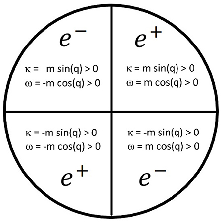
Figure 1. Bound states for electrons and positrons in an electrostatic δ-potential (λ = 0).
These bound states correspond to one positive energy electron trapped in either one positive or negative energy state and one positive energy positron trapped alternatively in positive or negative energy states. This structure is periodic in q.
Positron bound states
1. ; κb = m sin q > 0,
2. ; κb = −m sin q > 0,
Electron bound states
1. ; κb = m sin q > 0,
2. ; κb = −msin q>0,
It is worthwhile to mention that if or zero modes exist. For instance when we have κb = m, ωb = 0 whereas the eigenspinor reads:
We stress that the bound states just described are closer to the bound states in the scalar case with mixed potential of the form V(x) = −aδ(x)+bδ′(x) (see [23]). In both cases the normalizable wave functions exhibit finite discontinuities at the origin.
The charge density can be written as:
being Q a positive constant and taken into account that + will be chosen in the case of electrons and − for positrons. On the one hand, if we substitute the positron bound states (39, 40) in (43) the charge density obtained is
On the other hand, if we substitute the electron bound states (41, 42) in (43) the charge density obtained is
All the results are shown in Figure 2.
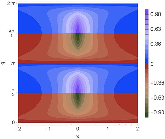
Figure 2. Charge density as a function of x when Q = m = 1 and λ = 0 (electrostatic δ-potential). For 0 < q < π/2 and π < q < 3π/2 the charge densities of a positron bound state are plotted [(44), (45), respectively]. For π/2 < q < π and 3π/2 < q < 2π the charge densities of a electron bound state are plotted [(46), (47), respectively].
We pass to study the scattering of 1D Dirac particles through a Dirac electrostatic δ-potential (V(x) = qδ(x)𝟙) in order to obtain the scattering amplitudes. On the one hand, electron scattering spinors coming from the left toward the δ-impurity (“diestro”scattering) have the form:
where u+(k) is the positive energy electron spinor that solves the free static Dirac equation for plane waves moving along the real line (23). The solutions in both zones are related at the origin through the electrostatic δ-matching conditions (10) if and only if the transmission and reflection scattering amplitudes are:
which obviously satisfy the unitarity condition: . On the other hand, electrons coming from the right toward the δ-impurity, (“zurdo”scattering), are described by spinors of the form
The δ-well matching conditions (10) for this “zurdo” scattering ansatz are satisfied if σR(k) = σL(k) and ρR(k) = ρL(k). It is worth noting that
• Since the scattering amplitudes for “diestro”and “zurdo”scattering of the electrons through an electrostatic δ-potential are identical, the processes governed by this potential are parity and time-reversal invariants.
• Purely imaginary poles k = iκ of the transmission amplitude σ are the bound states of the spectrum if κ is real and positive. In formula (49) we observe that poles of this type appear if the imaginary momentum satisfies the equation
which admits positive solutions for κb only if tan q < 0, i.e., if q lives in the second or fourth quadrant. Moreover, explicit solutions of the previous equation are: κb = ±m sin q, i.e., assuming that m > 0 the plus sign must be selected in the second quadrant and the minus sign is valid in the fourth quadrant.
• Probability is conserved even in this relativistic quantum mechanical context provided that ω2 > m2, m > 0.
For positrons, the “diestro”scattering ansatz of the spinor (that is a solution of the conjugate Dirac equation in zones I and II) is
where v+(k) is the positive energy positron spinor that represents plane waves moving along the real line (25). By imposing the matching conditions on x = 0 (18), the following scattering coefficients are obtained
Again, unitarity is preserved: .
The “zurdo”positron scattering ansatz, however, takes the form
Again, by imposing the matching conditions on x = 0 (18), we find that and . It is worth noting that
• The scattering amplitudes for “diestro” and “zurdo” scattering of positrons through an electrostatic δ-well are identical: there is no violation of parity and time reversal invariance in the scattering of positrons by δ-impurities.
• The purely imaginary k = iκ poles of are the positron bound states in the spectrum of the conjugate Dirac Hamiltonian. In formula (52) we observe that poles of this type appear if the imaginary momentum satisfies the equation
which admits positive solutions for κb only if tan q > 0, i.e., if q lives in the first or third quadrant. Between the explicit solutions of this equation, κb = ±msinq, the plus sign must be chosen in the first quadrant, and the minus sign in the third quadrant assuming that m > 0.
• The relations between diestro and zurdo scattering amplitudes for electrons and positrons are as follows:
The unitary S-matrix
encodes the phase shifts in its spectrum; . The phase shifts δ±(k) in the even and odd channels are thus
whereas the total phase shift δ(k) = δ+(k) + δ−(k) is easily derived:
Next, we consider the one-dimensional Dirac Hamiltonian with a single Dirac δ-potential disturbing the mass term:
Firstly, we will search for bound states where electrons and positrons are trapped by mass-spike δ wells. In the case of electrons, away from the singularity the positive energy spinors take the form (33, 34). The continuation to the whole real line is achieved by applying to those spinors the relativistic matching conditions at the origin x = 0 (12) as follows:
In this way, we obtain the following homogeneous algebraic system written in matrix form as:
The determinant of this 2 × 2 matrix is zero such that there is a non null solution of (56) if κb = −m tanh λ which provides a normalizable spinor only if λ < 0. The energy of the electron bound state is ωb = m sech λ. This bound state spinor is extended to the whole line by means of the condition , i.e., the spinor takes the form:
The charge density of this bound state is obtained by replacing the spinor (57) in the equation (43), arriving at the result
which is represented in Figure 3.
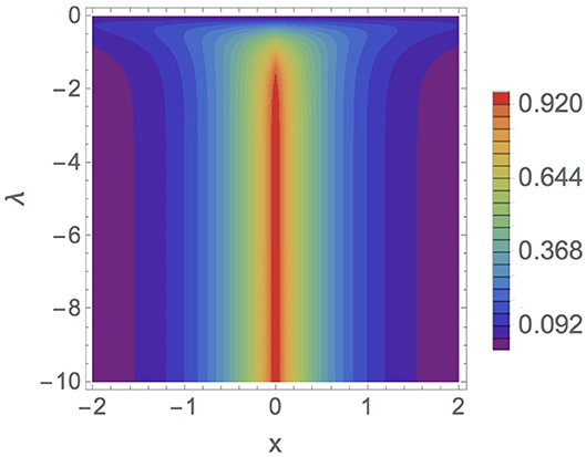
Figure 3. Charge density (58) as a function of x for electrons when Q = m = 1 and q = 0 (mass-spik δ-potential).
Investigation of positron bound states requires applying the same relativistic matching conditions (12) at the origin to the bound state positron spinors (36)–(37) in order to obtain the following homogeneous algebraic system written in matrix form as:
The determinant of this 2 × 2 matrix is zero such that there is a non null solution of (59) if κb = m tanh λ. This imaginary momentum provides a normalizable spinor only if λ>0. The energy of this positron bound state is ωb = m sech λ. The spinor bound state is extended to the whole line by means of the condition :
The charge density of this bound state is obtained by replacing the spinor (60) in the equation (43), arriving at the result
which is represented in Figure 4.
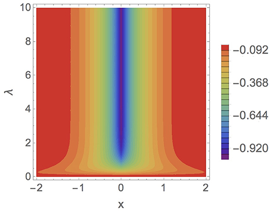
Figure 4. Charge density (61) as a function of x for positrons when Q = m = 1 and q = 0 (mass-spike δ-potential).
To obtain the scattering amplitudes for electrons coming from the left (“diestro”scattering) on mass-spike impurities the free spinors in zones I and II away from the origin (48) must be joined by using the 𝕊𝕌(1, 1) matrix appearing in (55). More explicitly, this matching sets an algebraic system whose solutions are the scattering coefficients:
which obviously respect probability conservation:
Repeating this procedure for the “zurdo”scattering spinorial ansatz (50) we conclude with the same relativistic δ-interaction scattering amplitudes as in “diestro”scattering. In sum
• The scattering amplitudes for diestro and zurdo scattering of electrons through a mass-spike δ-interaction are identical. This means that the mass-spike δ interaction respect both parity and time-reversal symmetries.
• The S-matrix is unitary and the phase shifts appear as the exponents of its eigenvalues. The total phase shift is:
• The purely imaginary poles of the transmission amplitude σ(k) with positive imaginary part are the bound states of the spectrum and occur when: kb = iκb = −im tanh λ, i.e., ωb = m sech λ. It must be fulfilled that tanh λ < 0.
Investigation of the positron “diestro”scattering amplitudes is achieved by imposing the relativistic matching conditions
on the positron spinor scattering ansatz (51). This criterion is tantamount to an algebraic system for the scattering amplitudes whose solutions are:
which also respects probability conservation:
To avoid repetitions, we skip a detailed computing of the positron scattering amplitudes for “zurdo”scattering, we merely states that are identical to the scattering amplitudes for positrons coming from the left toward the δ-obstacle. Thus, we summarize the main features of positron scattering through a mass-spike δ-imputity as follows:
• The scattering amplitudes for diestro and zurdo scattering of positrons through a mass-spike δ-interaction are identical to each other. Therefore, there is no breaking of either parity or time-reversal symmetries.
• The S-matrix is unitary and the phase shifts appears as the exponents of its eigenvalues. The total phase shifts for positrons are
• The purely imaginary poles of the transmission amplitude with positive imaginary part are the positron bound states of the spectrum and occur when kb = iκb = im tanh λ, i.e., ωb = m sech λ. It must be fulfilled that tanh λ > 0.
• The relations between diestro and zurdo scattering amplitudes for electrons and positrons in a mass-spike δ-potential are as follows:
The spectrum of the 1D Dirac Hamiltonian providing the one-particle spectrum for 1D electrons and positrons has been analyzed when there is one impurity that distorts the free propagation of fermions. We have implemented the impurity by means of Dirac δ-potentials of two types that we denote respectively as electrostatic and mass-spike according to their physical meaning.
In the electrostatic case (where the coupling is an angle) we find that:
1. There are two quadrants (π/2 < q < π and 3π/2 < q < 2π) where the coupling of the δ-interaction gives rise to one electron bound state. One positron bound state arise in the other two quadrants (0 < q < π/2 and π < q < 3π/2).
2. Regarding scattering amplitudes we found that positrons and electrons are scattered by the impurity so that the electron scattering coefficients are the conjugate of the positron ones.
For mass-spike δ-potentials our results are:
1. There is one bound state of electrons if the coupling is negative and other one of positrons if the coupling is positive.
2. The scattering amplitudes of electrons due to a mass-spike δ-impurity are the conjugate of positrons ones.
We plan to continue this investigation along the following lines of research:
• First, our purpose is to study the effect on free fermions of an impurity carrying both electrostatic and mass-spike couplings.
• Second, it is our intention to consider two, several or even infinity δ-impurities (often called as δ-comb potential), as the periodic potentials arise in various materials models.
• Third, after having managed all these tasks, we envisage to compute quantum vacuum energies and Casimir forces induced by these 1D fermions, in a parallel analysis to that performed for bosons in [17] and references quoted therein.
The raw data supporting the conclusions of this manuscript will be made available by the authors, without undue reservation, to any qualified researcher.
All authors listed have made a substantial, direct and intellectual contribution to the work, and approved it for publication.
The authors declare that the research was conducted in the absence of any commercial or financial relationships that could be construed as a potential conflict of interest.
JG, JM-C, and LS-S are grateful to the Spanish Government-MINECO (MTM2014-57129-C2-1-P) and the Junta de Castilla y León (BU229P18, VA137G18, and VA057U16) for the financial support. LS-S is grateful the Valladolid University, through the Ph.D. fellowships programme (Contratos predoctorales de la UVa). JM-C would like to thank M. Gadella, G. Fucci, M. Asorey, and L. M. Nieto for fruitful discussions. JM-C and LS-S acknowledge the technical computing support received by Diego Rogel.
1. ^We shall allow q to vary as an angle proportional to the fine structure constant, which in a 1D space is , the electron charge times the Compton particle wavelength to the square.
2. ^We shall refer as spinor fields to the Fermi fields even though in one-dimension there is no spin.
1. Aharonov Y, Bohm D. Significance of electromagnetic potentials in the quantum theory. Phys Rev. (1959) 115:485–91. doi: 10.1103/PhysRev.115.485
2. Jackiw R, Rebbi C. Solitons with fermion number 1/2. Phys Rev D. (1976) 13:3398–409. doi: 10.1103/PhysRevD.13.3398
3. Rubakov VA. Adler-Bell-Jackiw anomaly and fermion number breaking in the presence of a magnetic monopole. Nucl Phys. (1982) B203:311–48.
4. Alford MG, Wilczek F. Aharonov-Bohm interaction of cosmic strings with matter. Phys Rev Lett. (1989) 62:1071–4. doi: 10.1103/PhysRevLett.62.1071
5. Park DK, Oh JG. Self-adjoint extension approach to the spin-1/2 Aharonov-Bohm-Coulomb problem. Phys Rev D. (1994) 50:7715–20. doi: 10.1103/PhysRevD.50.7715
6. Andrade FM, Silva EO, Pereira M. Physical regularization for the spin-1/2 Aharonov-Bohm problem in conical space. Phys Rev D. (2012) 85:041701. doi: 10.1103/PhysRevD.85.041701
7. Jackiw R. Diverse Topics in Theoretical and Mathematical Physics. Singapore: World Scientific (1995).
8. Šeba P. Klein's paradox and the relativistic point interaction. Lett Math Phys. (1989) 18:77–86. doi: 10.1007/BF00397060
9. Benvegnù S, Dabrowski L. Relativistic point interaction. Lett Math Phys. (1994) 30:159–67. doi: 10.1007/BF00939703
10. Pankrashkin K, Richard S. One-dimensional Dirac operators with zero-range interactions: Spectral, scattering, and topological results. J Math Phys. (2014) 55:062305. doi: 10.1063/1.4884417
11. Jackiw R, Milstein AI, Pi SY, Terekhov IS. Induced current and Aharonov-Bohm effect in graphene. Phys Rev B. (2009) 80:033413. doi: 10.1103/PhysRevB.80.033413
12. Masir MR, Vasilopoulos P, Peeters FM. Magnetic Kronig–Penney model for Dirac electrons in single-layer graphene. New J Phys. (2009) 11:095009. doi: 10.1088/1367-2630/11/9/095009
13. Bordag M, Hennig D, Robaschik D. Vacuum energy in quantum field theory with external potentials concentrated on planes. J Phys. (1992) A25:4483–98.
14. Sundberg P, Jaffe RL. The Casimir effect for fermions in one dimension. Ann Phys. (2004) 309:442–58. doi: 10.1016/j.aop.2003.08.015
15. Lapidus IR. Relativistic one dimensional hydrogen atom. Am J Phys. (1983) 51:1036–8. doi: 10.1119/1.13445
16. Calkin MG, Kiang D, Nogami Y. Proper treatment of the delta function potential in the one dimensional Dirac equation. Am J Phys. (1987) 55:737–9.
17. Muñoz-Castañeda JM, Guilarte JM, Mosquera AM. Quantum vacuum energies and Casimir forces between partially transparent δ-function plates. Phys Rev. (2013) D87:105020. doi: 10.1103/PhysRevD.87.105020
18. Muñoz-Castañeda JM, Guilarte JM. δ-δ′ generalized Robin boundary conditions and quantum vacuum fluctuations. Phys Rev. (2015) D91:025028. doi: 10.1103/PhysRevD.91.025028
19. Bordag M, Muñoz-Castañeda JM. Quantum vacuum interaction between two sine-Gordon kinks. J Phys. (2012) A45:374012. doi: 10.1088/1751-8113/45/37/374012
20. Akcay H. Dirac equation with scalar and vector quadratic potentials and Coulomb-like tensor potential. Phys Lett A. (2009) 373:616–20. doi: 10.1016/j.physleta.2008.12.029
21. Hiller JR. Solution of the one-dimensional Dirac equation with a linear scalar potential. Am J Phys. (2002) 70:522–4. doi: 10.1119/1.1456074
22. Nogami Y, Toyama FM, van Dijk W. The Dirac equation with a confining potential. Am J Phys. (2003) 71:950–1. doi: 10.1119/1.1555891
Keywords: contact interactions, Dirac equation, Dirac delta, selfadjoint extensions, relativistic quantum mechanics
Citation: Guilarte JM, Munoz-Castaneda JM, Pirozhenko I and Santamaría-Sanz L (2019) One-Dimensional Scattering of Fermions on δ-Impurities. Front. Phys. 7:109. doi: 10.3389/fphy.2019.00109
Received: 22 March 2019; Accepted: 11 July 2019;
Published: 16 August 2019.
Edited by:
Luiz A. Manzoni, Concordia College, United StatesReviewed by:
Özlem Yeşiltaş, Gazi University, TurkeyCopyright © 2019 Guilarte, Munoz-Castaneda, Pirozhenko and Santamaría-Sanz. This is an open-access article distributed under the terms of the Creative Commons Attribution License (CC BY). The use, distribution or reproduction in other forums is permitted, provided the original author(s) and the copyright owner(s) are credited and that the original publication in this journal is cited, in accordance with accepted academic practice. No use, distribution or reproduction is permitted which does not comply with these terms.
*Correspondence: Juan Mateos Guilarte, Z3VpbGFydGVAdXNhbC5lcw==
Disclaimer: All claims expressed in this article are solely those of the authors and do not necessarily represent those of their affiliated organizations, or those of the publisher, the editors and the reviewers. Any product that may be evaluated in this article or claim that may be made by its manufacturer is not guaranteed or endorsed by the publisher.
Research integrity at Frontiers
Learn more about the work of our research integrity team to safeguard the quality of each article we publish.