Abstract
We review a controlled numerical approach to quantum impurity problems in realistic geometries, consisting of exactly mapping the complete lattice Hamiltonian onto an equivalent one dimensional system through a unitary transformation. The resulting dimensional and entanglement reduction allows one to study the quantum many-body problem on arbitrary d-dimensional lattices using the density matrix renormalization group (DMRG) method. The real-space resolution allows one to position the impurities at the boundary or bulk of the sample and to study screening effects due to edge or surface modes. We describe how to generalize this approach to multi-impurity problems, discuss applications and possible extensions.
1. Introduction
Research in engineering and fabrication of magnetic nano-structures has been, and continues to be, a fast growing field [1–5]. Their usefulness can potentially be applied to data storage, spintronics, sensors, magnetic imaging, quantum computing, and more [6]. Moreover, magnetic adatoms have been regarded as the building blocks of quantum nanostructures that can be assembled on crystal surfaces through single-atom manipulation with a scanning tunneling microscope (STM). These can serve as quantum simulators for studying magnetism with excellent real-space and energy resolution [7–9]. In the same spirit as cold-atom setups, this technique can unveil magnetic order and excitations in different geometries [10–13]. The surface not only supports the spin centers, but also plays a crucial role in stabilizing magnetic order [14–17]. Fundamental to all of these considerations is how individual spins interact with each other. Exchange interactions between impurities may have different physical origins: they can either arise from direct exchange for nearest-neighbor adsorption sites or indirect substrate-mediated coupling that asymptotically decay as a power-law with increasing separation between the impurities (Ruderman-Kittel-Kasuya-Yosida or RKKY interaction) [18–20].
The physics of a single magnetic impurity is well understood in terms of the Kondo problem: the magnetic moment is either partially or totally screened by the spin of the conduction electrons forming a collective many-body state with the Fermi sea [21]. In essence, the impurity ends up acting as a scattering center. However, in reality it is an extended object with a complex internal structure, usually referred-to as the hybridization cloud or “Kondo cloud,” which is centered at the impurity and decays with a characteristic range RK [22–24].
In order to understand how multiple impurities can realize magnetic order, it is first necessary to determine the effective interactions mediated by the conduction electrons in the substrate. A good point to start is by considering two Kondo impurities interacting locally with free fermions in the bulk via an antiferromagnetic exchange coupling JK [25]:
where Hband is the lattice Hamiltonian for non-interacting electrons, parameterized by a hopping t and represents the conduction electron's spin at the impurity's coordinate ri, for impurities i = 1, 2. The same form of the Hamiltonian can be generalized to multiple impurities.
Historically, the standard approach is to assume that the impurities see each-other via an effective RKKY interaction, or indirect-exchange. It was first introduced in 1954 by Rudderman and Kittel to explain the coupling of nuclear magnetic moments [19]. Kasuya realized the same method could be applied to localized d or f electrons in a metallic host [20] and further work was carried on by Yosida [18]. The problem can be thought of as one impurity interacting with the conduction electrons which then “carry” this interaction to the next impurity. The effective Hamiltonian in second order perturbation theory is written as:
where , is a distance dependent function and χ(R) is the Fourier transform of the non-interacting static susceptibility, or Lindhard function, which varies with distance, dimensionality and fermion density. The corresponding expression which is often cited in the literature is derived from assuming a uniform electron gas with a quadratic dispersion E(k) ~ k2 [26] and its asymptotic behavior at long distances (kFR ≫ 1) and in d dimensions is given by:
As multiple impurities are included, the problem is complicated by the fact that there are now competing energy scales. This perturbative approach ignores many important features such as the many-body physics that can lead to a Kondo ground state. Therefore, as we shall see, these arguments alone can not accurately describe multiple impurity physics at low temperatures.
As perturbative approaches fail for strongly interacting systems, numerical methods become essential for a better understanding of experimental results. In this review, we describe in detail a completely unbiased and controlled numerical approach to solve quantum impurity problems in d-dimensional lattices [27–29]. The method relies on an exact canonical transformation in which a Lanczos recursion allows one to recast the complete lattice Hamiltonian as a tri-diagonal matrix that in turn can be associated to an equivalent one dimensional tight-binding problem. This procedure can be recognized as a generalization of Wilson's numerical renormalization approach [30] and Haydock's recursion method [31–34]. After the non-interacting part of the problem has been reduced to a chain, the many-body physics is introduced in the form of a Kondo or Anderson impurity. The resulting low-dimensional problem can efficiently be solved using the density matrix renormalization group (DMRG) [35–38] method. We generalize these concepts to the multi-impurity case and discuss improvements to optimize the calculations in certain particular cases.
2. Mapping and Dimensional Reduction
2.1. Single Impurity
2.1.1. Lanczos Transformation
Solving for the ground state in an interacting lattice problem in dimensions greater than one is quite a challenging problem. Some impurity solvers include quantum Monte Carlo (QMC) [39–43] and the numerical renormalization group (NRG) [30, 44]. However, these methods have limitations, such as capturing the finite details of a lattice, or running into the well-known sign-problem (modern diagramatic QMC techniques somewhat overcome these issues). Fortunately, one-dimensional systems can be solved efficiently with the density matrix renormalization group (DMRG) technique [35–38]. This section is dedicated to transforming an d-dimensional non-interacting lattice Hamiltonian, onto an equivalent, solvable one-dimensional chain [27].
A general Hamiltonian for impurity problems will have the form
Here, Hl is a single-particle tight-binding Hamiltonian of a lattice. Himp and Vc describe the impurity and the coupling between impurity and lattice, respectively. We point out that this method is applicable regardless of the geometry or dimensionality of the lattice.
First, let one consider a single impurity problem and one orbital per site. More general cases of multiple orbitals and impurities will be discussed in the next section. We start by first considering the non-interacting band Hamiltonian without the impurity. In the presence of translational symmetry, this matrix can be readily diagonalized by transforming to a plane-wave basis. However, the impurity breaks this invariance but preserves other point group symmetries of the lattice, such as rotations and reflections. We would like to generate a single particle basis compatible with these. We get our inspiration from NRG: Wilson considered a free electron gas in the continuum and used a basis of partial waves centered at the position of the impurity. A lanczos transformation allowed him to map the problem onto an equivalent one dimensional chain that he solved by block decimation [30, 44] (NRG also introduces the idea of logarithmic discretization of energy scales and renormalization, that will not be used here). In our case, we carry out a similar procedure, but in the presence of the lattice. The intuition is as follows: consider a single electron state en real space representation corresponding to a particle at the lattice site connected to the impurity r0. By applying the non-interacting term of the Hamiltonian Hl we obtain a new state that is a superposition of single-particle states at the neighboring sites; this is the first “Lanczos orbital.” By continuing this procedure the wave-functions will expand radially outward, away from r0. However, the action of the hopping also makes these orbitals “contract” inward. In order to obtain an orthogonal basis, one needs to orthogonalize each new orbital with those obtained in prior iterations. This is precisely what the Lanczos recursion does for us. Formally, the procedure starts by choosing an appropriate single particle “seed” state as:
where creates an electron at site r0 and |0〉 is the vacuum state. This site can be chosen according to two situations. First, for a Kondo impurity, it is the site the impurity will couple to. Alternatively, for a substitutional impurity, typically described with an Anderson-type model, the seed is the impurity site (see Figure 1). As it will be made clear, the mapping does not effect the “seed” state and, therefore, does not modify Himp. In both cases, the mapping is performed in the same way.
Figure 1
Once the seed is chosen, the rest of the states are constructed with the following iterative procedure:
The equations for an and bn are obtained by requiring the states to be orthogonal. Note, however, that at this stage the states are not normalized.
After this transformation, Hl is tri-diagonal and has the form:
Equivalently, in second quantization it reads
where , are normalized creation and annihilation operators, respectively, is the particle number operator and L is the total length of the chain. The geometry of this new Hamiltonian is a chain as in Figure 1. The diagonal an terms are on-site potentials, while the bn's are the new hoppings along the chain.
While performing this recursion in practice, numerical errors are introduced for large L due to finite precision. There are two ways to reduce these errors: (1) Since 〈Ψn|Ψn〉 grows with n, normalize Ψn−1 at each iteration. (2) To prevent loss of orthogonalization, introduce re-orthogonalization. This can easily done with the following procedure:
As an example, consider a 2D square lattice of linear dimension L. Instead of L2 sites, one now has to keep only ~ O(L) sites. This is indeed an exact canonical transformation. The remaining missing orbitals correspond to different symmetry sectors of the Hamiltonian and consequently are completely decoupled from the impurity. The impurity is only coupled to the “s-wave” channel. The seed site acts as center of symmetry for the group D4h. The “s-wave” channel corresponds to the totally symmetric representation A1g and is formed by the basis function {x2 + y2}. Different symmetry channels corresponding to different representations such as those shown in Figure 2 will form their own independent chains. An example of this is the B1g representation formed by the {x2 − y2} basis function which can be thought of as a “d-wave” channel. The key point of this mapping is that it leaves Himp and Vc in Equation (3) unchanged after the transformation. The first site of the chain corresponds to a real lattice site in real space. Therefore, as mentioned, the impurity will only couple to this single site of the chain.
Figure 2
If the lattice is infinite, the recursion can be performed indefinitely. In practice, the iterations are stopped and the chain is cut after some sufficient number of iterations. This is equivalent to assuming the lattice has the same “shape and size” as the last orbital in the Lanczos iteration. Alternatively, one can consider a finite lattice of arbitrary shape. Once the boundary is reached by the orbitals, they will “bounce” or reflect back, retracing the path to the seed site. At some point, we will find that bn+1 = 0, meaning that all orbitals within that symmetry sector have been exhausted and we have a chain of finite length. If the finite lattice has no symmetry elements, the chain length will be equal to the total number of lattice sites. For instance, for the case of a square lattice, Lanczos orbitals for a single impurity have a diamond-like shape (see Figure 1). If the lattice has a boundary with a different symmetry, the different symmetry sectors will mix.
The full many body problem is recovered by connecting the impurity back to the chain. The recursion has not affected the terms Himp and Vc in Equation (3), so the impurity will now be connected to the first site of the chain (the seed orbital) by Vc without any changes. These Hamiltonian can now be solved with DMRG, or any method of choice.
2.1.2. Entanglement Reduction
As previously described, the Lanczos orbitals are defined by their symmetry properties, or channel, and their radial distance from the center of symmetry, which can be associated to the linear distance along the equivalent one-dimensional chain. These considerations provide for an intuitive understanding of the scaling of the entanglement. In the equivalent problem after the Lanczos transformation, the region enclosed by an area of “radius” L in the d-dimensional lattice maps onto ~ Ld−1 one-dimensional chains, each corresponding to a different symmetry sector. The entanglement per channel between this region and the rest of the lattice is exactly the same as the entanglement between the first L sites of each chain and their complement. In cases where the system under consideration is gapless, the chain is a critical one-dimensional system (for square and cubic lattices, for instance) and the von Neumann entanglement entropy is proportional to log(L) [45, 46]. All channels contribute to the entropy with similar factors. This yields a final result proportional to Ld−1 log(L). These simple arguments easily explain why free fermions in higher-dimensions have logarithmic corrections to the area law [47–50]. Remarkably, one only needs to solve the problem in the channel that is directly coupled to the impurity, reducing the entanglement by a factor of Ld−1!
2.1.3. Continued Fractions and Non-interacting Green's Functions
The Lanczos transformation described above can be used to obtain non-interacting Green's Functions (GF). As a matter of fact, it was originally introduced in the literature with this purpose and it is known as the continued fraction expansion, or method of the moments [31–34]. Consider the Green's Function,
Define a projection operator as P0 = |Φ0〉〈Φ0|, where |Φ0〉 is our seed state of the mapping. The projected GF is then defined as
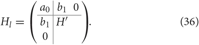
Now, it is clear that the function G0(ω) is just the 00 element of the matrix (ωÎ − Ĥ)−1, where Ĥ is the tri-diagonal Hamiltonian after the Lanczos transformation as in Equation (9). To compute this inverse, it is best to partition the matrix into blocks, then utilize properties of partitioned matrices. For example, an m × m matrix of the form:
where a is a scalar, b is an (m − 1) × 1 vector and C is an (m − 1) × (m − 1) matrix. Then the 00 entry is given by,
In the current case, bT is just (b1, 0, 0, 0, … ), so the above equation reduces to, switching back to the an and bn notation of Equation (9):
The process is then repeated for . This method can be used to find any matrix element of G(ω). After iterating, the result is a continued fraction:
Recall that |ϕ0〉 represents a site in real space of the lattice. The density of states (DOS) and local density of states (LDOS) for a system are defined, respectively as,
The LDOS of any geometry can then be computed numerically. Notice the first site of the chain has the exact DOS of the lattice. One way to terminate the expansion is just to cut the chain at some sufficient chain length n, as in Equation (17). However, this results in poor resolution of the LDOS, even for quite large n. Instead, consider a continued fraction with all an and bn constant, i.e., an = a and bn = b for all n. The continued fraction, after an equivalence transform can be written as
where and the continued fraction is carried out indefinitely. This expression converges to a finite value for all complex z with finite imaginary part. This value is given by
Using the square lattice again for an example, the hoppings bn along the Lanczos chain converge to b∞ = 2 as seen in Figure 3A. After a sufficient number of iterations, the values of an and bn are approaching their asymptotic limits. This permits the insertion of the expression Y(z) into the continued fraction yielding the desired result,
Doing so, results in the ability to take the limit δ → 0, resulting in a well resolved LDOS as seen in Figure 3B.
Figure 3
This method can be generalized to the case when bn is alternating between two or more values. This can happen if there is a gap in the band structure, such as when there are different on-site energies for opposite sublattices of a bipartite lattice. The continued fraction is then considered periodic and a similar but slightly more complicated expression can be found for Y(z).
2.2. Multiple Impurities
2.2.1. Block Lanczos
In this section, an extension of the previous method based on the block Lanczos transformation [51, 52] for multiple orbital or multi-impurity problems will be presented, following the original work in Shirakawa and Yunoki [29] and Allerdt et al. [28]. These considerations apply to different orbitals of the same atom, or impurities sitting at different lattice sites. As before, the first step is to choose the seed states. For illustrative purposes, let us consider a square lattice with two seeds at positions r1 and r2, defined as:
with the additional requirement that 〈α0|β0〉 = 0. Once the seeds are chosen, a new set of states can be obtained through the block Lanczos method [53]. The idea is the same: apply the Hamiltonian to each state and require orthogonality. The new set of states can be found through the iterative procedure as
By requiring the states |αn〉, |βn〉 to be orthogonal to all |αk<n〉, |βk<n〉, the a and b coefficients can be found by solving the following matrix equations:
A solution to these is ensured by the fact that 〈αn|αn〉 ≠ 〈αn|βn〉. The block Lanczos recursion will result in the geometry of a ladder as shown in Figure 4. Note that the states are not normalized at this stage. An important aspect of this method is that states within the same block are not generally orthogonal, i.e., 〈αn|βn〉 ≠ 0 (resulting in the vertical rung coupling in the ladder). Since we are interested in an orthonormal basis, we can use a Gram Schmidt procedure—although there are many ways—, to orthogonalize them. This is done by choosing
which will also simplify the geometry causing some hoppings in the ladder to vanish. If the seed orbitals are spatially separated such that the Lanczos orbitals have not yet met or overlapped, the hoppings connecting the legs of the ladder will remain zero and the hoppings along the chain will be equal to the single seed case.
Figure 4
Our Hamiltonian can now be written in the desired tridiagonal form:
where An and Bn are 2 × 2 matrices. These ideas can readily be generalized to an arbitrary number of impurities. For k impurities, each A and B matrix will be k × k. As long as the initial states are orthogonal, a new set of states can be found as
This matrix represents a new non-interacting tight-binding Hamiltonian where each block becomes a “unit cell” (there is no-translational invariance in this case, though).
Intuitively, we can understand this geometry as follows: if the impurities are far apart, we can imagine performing independent single-impurity mappings for each of them that yield two decoupled one-dimensional chains. At some point, when the length of the chains is about half the separation distance between impurities, the orbitals interfere and orthogonality is lost. Therefore, after re-orthogonalizing them, we end up introducing mixing that translates into a hopping term between the chains, leading to the resulting ladder.
For k impurities, it can be recognized as k coupled chains forming a k × L ladder. The new geometry is now quasi one-dimensional.
2.2.2. Symmetric and Anti-symmetric Channels
In the presence of inversion symmetry, the legs of the ladder can be decoupled into independent chains [28]. This method can be employed in two-impurity problems on simple lattices such as square, hexagonal, cubic, triangular, etc. An example of when it can not be used is for Bernal stacked graphene when the seeds are both on A-sites of opposite layers. Following Allerdt et al. [28], the first step is to choose the initial seed states. This symmetrization is similar to a folding transformation used in bosonization and NRG [54–58] and is carried out by choosing symmetric and antisymmetric (or bonding and anti-bonding) combinations of the original single particle states. For two seeds at r1 and r2, they read:
Once the initial states are constructed, the Lanczos recursion is identical to the one seed case. The procedure is carried out for each initial state yielding two completely independent and orthogonal chains. Only after the impurities are introduced are these chains coupled. The resulting geometry is shown in Figure 5 including the impurities. This transformation however, does not leave Vc unchanged. We illustrate it for the case of the two-impurity Kondo model introduced above in Equation (1). To write the many-body terms of the Hamiltonian in the new basis we use the inverse transformation,
where , are defined in Equations (31) and (32), respectively, and the fact that
one arrives at the transformed Hamiltonian:
By applying this symmetry, not only the recursion is greatly simplified, but also that the equivalent problem reduces from a ladder to a chain. Since the real space entanglement on a chain is half of that on the ladder, this results into an exponential gain that dramatically improves the efficiency of the DMRG simulations.
Figure 5
2.3. Star Geometry
In certain cases, it can be beneficial to transform from a chain to a star geometry. It was recently shown that a star geometry results in lower ground state entanglement than the chain [59], making it ideal for DMRG calculations.
The single impurity case is presented here and same considerations can easily be extended to multiple impurities. This mapping corresponds to a second unitary transformation on top of the original lattice-to-chain conversion. In order to do this mathematically and numerically, the matrix Hl is split into two blocks (similar to the partition when calculating the LDOS with the continued fractions). One contains just the seed state, which remains unaltered and the other block contains the rest. Explicitly, Equation (9) is split into
The block corresponding to the non-interacting chain H′ is then diagonalized. The couplings to the seed site are then , where are the values of the nth eigenvector of H′ on the site (or the second site of the chain). Equation (36) then becomes
where a0 corresponds seed of the Lanczos transformation and the center sites in Figures 6A,B. The new bath energies ϵn are just the eigenvalues of H′.
Figure 6
To extend this idea to two impurities is straight forward. The Hamiltonian after the Lanczos transformation is again split into blocks, where now the first block contains both seed states. Obtaining the new hoppings and bath energies is identical to the single impurity case. The new form of Equation (29) will then be
The resulting geometry is shown in Figure 7. Depending on the symmetry of the lattice and impurities, certain Vn's will vanish, as in the case where the symmetric/antisymmetric seeds are used. Here, the most general form is shown.
Figure 7
In some circumstances, the impurities entangle strongly to some states in the metallic substrate within a window of width ~ JK around the Fermi energy, while a large fraction remains disentangled. When this occurs, it is convenient to use the star geometry, which allows one to reach extremely large systems, practically in the thermodynamic limit. The advantage here is that after the transformation to the star, some bath sites (in the interacting problem) will be double occupied and some will be empty. Observing that these states play no role in the physics, they can be safely discarded. For an application we refer the reader to Allerdt et al. [60].
3. DMRG Simulations
In the block Lanczos approach, the equivalent problem consists of a ladder with k legs, where k is the number of impurities. As discussed above, by means of a folding transformation one can reduce the entanglement by a factor of 2, with the consequent reduction in the number of DMRG states needed in the calculation. Typically, for S = 1/2 impurities we take a total system size to be L = 4n (including impurities), such that each impurity can form part of a collective RKKY state or its own Kondo cloud (it has been already observed that Kondo does not develop in chains of length L = 4n + 2 [61]). For instance, L = 204 corresponds approximately to a “sphere” around the two impurities of radius ~ 100. As explained above and described in Büsser et al. [27], we assume that the lattice has the same shape/symmetry as the orbitals. When this is the case, orbitals never “bounce back” inward and the Lanczos recursion can be stopped at an arbitrary number of iterations without introducing any bias. Typically, we consider system sizes at least 4 times larger than the maximum inter-impurity distance. Notice that each impurity configuration will generate a new mapping and the shape of the lattice will be modified as a consequence, depending on the relative position of the impurities and the number of Lanczos iterations. This could potentially lead to artifacts and care must be taken to make sure that no finite size effects are introduced.
Since the energy difference between the ground-state and the first excited state can be very small (~ 10−6), we fix the truncation error at 10−9 in all simulations. This translates into a number of DMRG states of the order of 3,000 or more in most cases. Achieving this level of accuracy in a ladder geometry (without the bonding-antibonding symmetrization) would be practically impossible due to the larger entanglement. However, as previously pointed out, it is possible to work in the star geometry directly. This is particularly ideal in the strong coupling limit, since the impurity is mostly entangled to an electron at position r0. The rest of the free electrons remain disentangled and, in “momentum” (or energy) space, they practically form a product state. In this basis, the number of states required to achieve the same accuracy is reduced dramatically.
4. Energy Scales
As suggested by Doniach [62] (see also [63]), one could define a binding energy (or “Kondo temperature”) for forming a Kondo singlet , or an RKKY state, and a competition between these two energy scales will dictate which phase will win. Another consideration that plays an important role in finite systems is the energy level spacing Δ that introduces another competing energy scale which can become significant in, for example, quantum dots [64]. The Kondo effect in small or confined systems has been referred to as the “Kondo Box.” It is expected that Δ will dominate the physics when TK ~ Δ. Large amounts of work have been dedicated to studies of the competition between TK and Δ, which is a complicated problem, as well as scaling in the presence of finite bandwidth [65]. A fully developed resonance (fully screened impurity) requires a finite density of states at the Fermi level. In this regime, even/odd effects in chain length and particle number are also observed [63, 66].
In order to understand the relevance of these scales in numerical simulations we first analyze the single impurity case at zero temperature. According to renormalization group arguments, the system flows to a strong coupling fixed point characterized by a single energy scale—the Kondo temperature TK. In this regime, the impurity and the conduction electrons form a scattering state, the “Kondo cloud,” that has a characteristic extension RK [22–24, 67–70] that depends on JK (or TK). At distances of the order of RK electrons are more entangled to the impurity. In finite systems where the conduction electrons are confined to a “Kondo box” [64, 71–74] all the electrons may all be inside the Kondo cloud, without an “outside.” This regime would correspond to the “crossover” between weak coupling and strong coupling in the RG flow.
The strong coupling limit can be explicitly realized by taking JK ≫ W, where W is the bandwidth, and physically results into a tightly bound singlet formed by the impurity and a localized electron at r0. This corresponds to RK = 0. As JK is reduced, the impurity will become correlated with electrons farther and farther from it and RK will increase. If the system is finite, at some point we will find RK ~ L and the Kondo singlet will extend to the entire volume and the impurity will couple mostly to one electron at the Fermi level. According to the analysis presented in Yang and Feiguin [75], practically a single conduction electron is responsible for most of the screening: In the weak-coupling limit, this electron is precisely at the Fermi level [63], while in the strong-coupling limit, it corresponds to the localized orbital directly in contact with the impurity spin. In both cases, the remaining conduction electrons form a completely disentangled Fermi sea. As a consequence, it is important in finite systems to have a single occupied state at the Fermi energy in order to realize screening (otherwise, the impurity will behave as a local moment, decoupled from the Fermi sea). This situation, however, is far from the universal, strong coupling regime [65].
To make these observations more explicit, we study the behavior of gap Δ0 to the first (triplet) excited state as a function of system size. We focus our discussion at JK = 1, where the effects are more obvious. In the thermodynamic limit the system is gapless, Δ0 → 0 as L → ∞: it costs no energy to flip a spin infinitely far from the impurity. In addition, we introduce the “correlation gap,” defined as:
The first term is a variational energy obtained by flipping the spin of the impurity with the operator. This action will disentangle the impurity from the chain and destroy the Kondo singlet. Equivalently, one could apply the operator to transform the Kondo singlet into a “Kondo triplet.” Both quantities are equivalent in the SU(2) symmetric case. This estimate will yield what we identify as the minimum energy cost for destroying the Kondo state, which can also be related to the Kondo temperature.
For small systems the energy spacing Δ is large and the gap Δ0 is determined by the correlation gap ΔK. As we increase the size of the Fermi sea, the level spacing is reduced and, at some point, Δ will become smaller than the correlation gap. When this happens, the system gap Δ0 follows the behavior of the level spacing and shrinks as 1/L, as clearly observed in Figure 8: the system undergoes a crossover from the weak Kondo-box-like regime to the universal strong coupling regime and ΔK becomes a system-independent characteristic energy scale.
Figure 8
One way to reach this regime in finite systems is by introducing “damped boundary conditions” [76]. In this particular case, we multiply the hoppings by a factor λ−n/2, where λ is a number larger than one and n is the position along the chain, counting from Lb sites before the boundary (we pick Lb = 15 in this case). This is reminiscent of Wilson leads, which have been successfully used in a number of contexts (besides NRG calculations) and are known to alleviate finite-size effects [77, 78] by making the energy spacing smaller around the Fermi energy. To illustrate this behavior we also show Δ, Δ0 and ΔK for different system sizes and JK = 1. We find that, as long as the “bulk” level spacing is large (for λ = 1), the gap Δ does not depend on the chain length, but only on λ and Lb (which is kept constant). Therefore, now one needs to focus on the behavior of the different quantities with λ and not L. As we see, for all values of λ considered here Δ is smaller than ΔK and is practically equal to Δ0. In addition, we see that while Δ gets smaller with increasing λ, the correlation gap ΔK stays constant, indicating that this is basically a measure of the correlation energy in the thermodynamic limit.
In the multi-impurity problem the correlation gap cannot distinguish between Kondo or RKKY physics and the origin of the correlation effects. In the two-impurity case, one compares ΔK against twice the value for a single impurity. The difference indicates the energy gained by forming a correlated RKKY state vs. to the one gained by two independent Kondo singlets.
5. Applications
The single impurity mapping can be used to study Kondo physics on graphene [79] or multi-band problems such as phosphorene, for instance [80]. It was found that, in the case of graphene, edge states tend to hybridize with the impurity spin introducing a competition between bulk and edge-induced Kondo screening.
The multi-impurity version allows one to explore a broad range of interesting open problems. Although briefly suggested in Büsser et al. [27], the block Lanczos method was formally introduced in Shirakawa and Yunoki [29] to study spin-spin correlations between an impurity and conduction electrons in graphene. The folding transformation was later used to investigate the competition between Kondo and RKKY physics on different geometries with small [28] and large spin [81] and a number of surprising results were found. Notably, there are important non-perturbative effects that in some cases make Kondo more robust than an RKKY state, even at short distances [28] of the order of a few lattice sites. This is a consequence of lattice effects that make the RKKY interaction very weak when impurities are sitting at positions where single particle wave-functions interfere destructively. See for instance Figure 1, the single particle wave functions that expand away from the impurity site have very small amplitude on the opposite sublattice, hindering the possibility of mediating an RKKY exchange interaction between impurities. Moreover, due to the fast decay of the RKKY interaction, Kondo screening becomes the dominant effect at relatively short inter-impurity separation. Interestingly, in the spin-1 problem, it was found that impurities can be practically screened by the substrate, while simultaneously forming an RKKY state [81].
The method is particularly suited to study the structure of the correlations around a single impurity. In this case, one seed site is connected to the impurity and the second one is used to measure the two-point correlations between the conduction electron in the substrate and the impurity spin [29]. For instance, one could place the impurity at the edge or bulk of the material and calculate the correlations around substitutional impurities and adatoms at the edge of a topological insulator [82, 83]. Unlike previous calculations that consider the coupling of the impurity to one-dimensional effective modes [84, 85], in this formulation the helical liquid arises naturally as an edge effect of the two-dimensional bulk. Similarly, one could place the impurity on metallic (111) surfaces and study the influence of bulk states and Shockley surfaces states on the RKKY interaction [60].
Remarkably, this approach can be extended to a one-dimensional interacting “wire” connected to a substrate [86, 87]. The many-body physics in this case is contained in the wire (for instance, a Hubbard chain), while the substrate remains non-interacting. The mapping leads to Lanczos orbitals that describe cylindrical “shells” centered at the wire as their axis of symmetry. The generalization takes advantage of the translational invariance of the system along the wire direction that results into the wire being connected to an array of independent semi-infinite 1D chains, each characterized by a momentum kx. In this representation the chain Hamiltonian becomes non-local due to the interaction terms. Other mappings are possible, mixing real-space and momentum representation. It is convenient to preserve the locality of the interaction terms in the chain by using the real-space representation of it. As a price, the tunneling terms between the chain and the substrate become non-local. In the case of an insulating substrate, the length of the chains can be truncated and the system can be solved with the DMRG.
6. Conclusions
We have discussed a powerful method to study multi-impurity problems in realistic lattice geometries and configurations. This approach can readily be generalized to study generic band structures, multi-orbital problems, and magnetic molecules. It can be used in conjunction with first-principles band structure calculations, where the information about the metallic substrate is calculated using density functional theory. Quantum chemistry methods such as CASPT2 or NEVPT2 can be used to precisely calculate the hybridization terms in the structure of the seed state, paving the way toward a first principles modeling and a better understanding of correlation effects in quantum impurity problems.
We point out that any quadratic Hamiltonian can be mapped onto an equivalent one-dimensional system following this prescription, including problems with spin-orbit interaction, disorder and superconductors (at the mean field/BdG level).
Although the DMRG method was used as a solver for the effective one-dimensional impurity Hamiltonian, other methods are equally applicable, such as the embedded cluster approximation [24] or quantum Monte Carlo. One could also use these techniques to study time-dependent [88, 89] and thermodynamic properties [90], or to calculate spectral functions [91, 92].
Statements
Author contributions
All authors listed have made a substantial, direct and intellectual contribution to the work, and approved it for publication.
Acknowledgments
The work at Northeastern University was supported by the US Department of Energy (DOE), Office of Science, Basic Energy Sciences grants number DE-SC0014407.
Conflict of interest
The authors declare that the research was conducted in the absence of any commercial or financial relationships that could be construed as a potential conflict of interest.
References
1.
ObergJCCalvoMRDelgadoFMoro-LagaresMSerrateDJacobDet al. Control of single-spin magnetic anisotropy by exchange coupling. Nat Nano. (2013) 9:64–8. 10.1038/nnano.2013.264
2.
GambardellaPRusponiSVeroneseMDhesiSSGrazioliCDallmeyerAet al. Giant magnetic anisotropy of single cobalt atoms and nanoparticles. Science. (2003) 300:1130–3. 10.1126/science.1082857
3.
TaoKStepanyukVSBrunoPBazhanovDIMaslyukVVBrandbygeMet al. Manipulating magnetism and conductance of an adatom-molecule junction on a metal surface: an ab initio study. Phys Rev B. (2008) 78:014426. 10.1103/PhysRevB.78.014426
4.
SerrateDFerrianiPYoshidaYHlaSWMenzelMvon BergmannKet al. Imaging and manipulating the spin direction of individual atoms. Nat Nano. (2010) 5:350–3. 10.1038/nnano.2010.64
5.
WarnerBEl HallakFPrüserHSharpJPerssonMFisherAJet al. Tunable magnetoresistance in an asymmetrically coupled single-molecule junction. Nat Nano. (2015) 10:259–63. 10.1038/nnano.2014.326
6.
NalwaHS editor. Magnetic Nanostructures. Valencia, CA: American Scientific Publishers (2009).
7.
HeinrichAJGuptaJALutzCPEiglerDM. Single-atom spin-flip spectroscopy. Science. (2004) 306:466. 10.1126/science.1101077
8.
OtteAFTernesMLothSLutzCPHirjibehedinCFHeinrichAJ. Spin excitations of a kondo-screened atom coupled to a second magnetic atom. Phys Rev Lett. (2009) 103:107203. 10.1103/PhysRevLett.103.107203
9.
SpinelliARebergenMPOtteAF. Atomically crafted spin lattices as model systems for quantum magnetism. J Phys. (2015) 27:1–17. 10.1088/0953-8984/27/24/243203
10.
HirjibehedinCFLutzCPHeinrichAJ. Spin coupling in engineered atomic structures. Science. (2006) 312:1021. 10.1126/science.1125398
11.
KhajetooriansAAWiebeJChilianBLounisSBlügelSWiesendangerR. Atom-by-atom engineering and magnetometry of tailored nanomagnets. Nat Publishing Group. (2012) 8:497–503. 10.1038/nphys2299
12.
SpinelliABryantBDelgadoFFernández-RossierJOtteAF. Imaging of spin waves in atomically designed nanomagnets. Nat Mater. (2014) 13:782–5. 10.1038/nmat4018
13.
ToskovicRvan den BergRSpinelliAEliensISvan den ToornBBryantBet al. Atomic spin-chain realization of a model for quantum criticality. Nat Phys. (2016) 12:656–60. 10.1038/nphys3722
14.
StepanyukVSNiebergallLLongoRCHergertWBrunoP. Magnetic nanostructures stabilized by surface-state electrons. Phys Rev B. (2004) 70:075414. 10.1103/PhysRevB.70.075414
15.
ZhouLWiebeJLounisSVedmedenkoEMeierFBlugelSet al. Strength and directionality of surface Ruderman-Kittel-Kasuya-Yosida interaction mapped on the atomic scale. Nat Phys. (2010) 6:187–91. 10.1038/nphys1514
16.
IgnatievPANegulyaevNNSmirnovASNiebergallLSaletskyAMStepanyukVS. Magnetic ordering of nanocluster ensembles promoted by electronic substrate-mediated interaction: \textit{Ab initio} and kinetic Monte Carlo studies. Phys Rev B. (2009) 80:165408. 10.1103/PhysRevB.80.165408
17.
WahlPSimonPDiekhönerLStepanyukVSBrunoPSchneiderMAet al. Exchange interaction between single magnetic adatoms. Phys Rev Lett. (2007) 98:056601. 10.1103/PhysRevLett.98.056601
18.
YosidaK. Magnetic properties of Cu-Mn alloys. Phys Rev. (1957) 106:893–8. 10.1103/PhysRev.106.893
19.
RudermanMAKittelC. Indirect exchange coupling of nuclear magnetic moments by conduction electrons. Phys Rev. (1954) 96:99–102. 10.1103/PhysRev.96.99
20.
KasuyaT. A Theory of Metallic Ferro- and Antiferromagnetism on Zener's Model. Prog Theor Phys. (1956) 16:45–57. 10.1143/PTP.16.45
21.
HewsonAC. The Kondo Problem to Heavy Fermions. Cambridge: Cambridge University Press (1997).
22.
SørensenESAffleckI. Scaling theory of the Kondo screening cloud. Phys Rev B. (1996) 53:9153–67. 10.1103/PhysRevB.53.9153
23.
AffleckI. The Kondo screening cloud: what it is and how to observe it. In: Aharony A, Entin-Wohlman O, editors. Perspectives on Mesoscopic Physics: Dedicated to Professor Yoseph Imry's 70th Birthday. Singapore: World Scientific (2010). p. 1–44.
24.
BüsserCAMartinsGBRibeiroLCVernekEAndaEVDagottoE. Numerical analysis of the spatial range of the Kondo effect. Phys Rev B. (2010) 81:045111. 10.1103/PhysRevB.81.045111
25.
JayaprakashCKrishna-murthyHRWilkinsJW. Two-impurity kondo problem. Phys Rev Lett. (1981) 47:737–40. 10.1103/PhysRevLett.47.737
26.
AristovDN. Indirect RKKY interaction in any dimensionality. Phys Rev B. (1997) 55:8064–6. 10.1103/PhysRevB.55.8064
27.
BüsserCAMartinsGBFeiguinAE. Lanczos transformation for quantum impurity problems in d-dimensional lattices: application to graphene nanoribbons. Phys Rev B. (2013) 88:245113. 10.1103/PhysRevB.88.245113
28.
AllerdtABüsserCAMartinsGBFeiguinAE. Kondo versus indirect exchange: role of lattice and actual range of RKKY interactions in real materials. Phys Rev B. (2015) 91:085101. 10.1103/PhysRevB.91.085101
29.
ShirakawaTYunokiS. Block Lanczos density-matrix renormalization group method for general Anderson impurity models: application to magnetic impurity problems in graphene. Phys Rev B. (2014) 90:195109. 10.1103/PhysRevB.90.195109
30.
WilsonKG. The renormalization group: critical phenomena and the Kondo problem. Rev Mod Phys. (1975) 47:773. 10.1103/RevModPhys.47.773
31.
HaydockRHeineVKellyM. Electronic structure based on the local atomic environment for tight-binding bands. J Phys C. (1972) 5:2845. 10.1088/0022-3719/5/20/004
32.
HaydockRHeineVKellyM. Electronic structure based on the local atomic environment for tight-binding bands. II. J Phys C. (1975) 8:2591. 10.1088/0022-3719/8/16/011
33.
HaydockR. The recursive solution of the Schrödinger equation. Comput Phys Commun. (1980) 20:11–6. 10.1016/0010-4655(80)90101-0
34.
ViswanathVSMüllerG. The Recursion Method: Application to Many Body Dynamics. Berlin; Heidelberg: Springer (1994). 10.1007/978-3-540-48651-0
35.
WhiteSR. Density matrix formulation for quantum renormalization groups. Phys Rev Lett. (1992) 69:2863–6. 10.1103/PhysRevLett.69.2863
36.
WhiteSRNoackRM. Real-space quantum renormalization groups. Phys Rev Lett. (1992) 68:3487–90. 10.1103/PhysRevLett.68.3487
37.
WhiteSR. Density-matrix algorithms for quantum renormalization groups. Phys Rev B. (1993) 48:10345–56. 10.1103/PhysRevB.48.10345
38.
SchollwöckU. The density-matrix renormalization group. Rev Mod Phys. (2005) 77:259. 10.1103/RevModPhys.77.259
39.
HirschJEFyeRM. Monte Carlo method for magnetic impurities in metals. Phys Rev Lett. (1986) 56:2521–4. 10.1103/PhysRevLett.56.2521
40.
GubernatisJEHirschJEScalapinoDJ. Spin and charge correlations around an Anderson magnetic impurity. Phys Rev B. (1987) 35:8478. 10.1103/PhysRevB.35.8478
41.
WernerPComanacAdeMediciLTroyerMMillisAJ. Continuous-time solver for quantum impurity models. Phys Rev Lett. (2006) 97:076405. 10.1103/PhysRevLett.97.076405
42.
GullEWernerPParcolletOTroyerM. Continuous-time auxiliary-field Monte Carlo for quantum impurity models. Europhys Lett. (2008) 82:57003. 10.1209/0295-5075/82/57003
43.
GullEMillisAJLichtensteinAIRubtsovANTroyerMWernerP. Continuous-time Monte Carlo methods for quantum impurity models. Rev Mod Phys. (2011) 83:349. 10.1103/RevModPhys.83.349
44.
BullaRCostiTAPruschkeT. Numerical renormalization group method for quantum impurity systems. Rev Mod Phys. (2008) 80:395. 10.1103/RevModPhys.80.395
45.
CalabresePCardyJ. Entanglement entropy and quantum field theory. J Stat Mech. (2004) 2004:P06002. 10.1088/1742-5468/2004/06/P06002
46.
CalabresePCardyJ. Entanglement entropy and quantum field theory: a non-technical introduction. Int J Quantum Inf. (2006) 4:429. 10.1142/S021974990600192X
47.
WolfMM. Violation of the Entropic Area Law for Fermions. Phys Rev Lett. (2006) 96:010404. 10.1103/PhysRevLett.96.010404
48.
GioevDKlichI. Entanglement entropy of fermions in any dimension and the widom conjecture. Phys Rev Lett. (2006) 96:100503. 10.1103/PhysRevLett.96.100503
49.
LiWDingLYuRRoscildeTHaasS. Scaling behavior of entanglement in two- and three-dimensional free-fermion systems. Phys Rev B. (2006) 74:073103. 10.1103/PhysRevB.74.073103
50.
BarthelTChungMCSchollwöckU. Entanglement scaling in critical two-dimensional fermionic and bosonic systems. Phys Rev A. (2006) 74:022329. 10.1103/PhysRevA.74.022329
51.
CullumJKWilloughbyRA. Lanczos Algorithms for Large Symmetric Eigenvalue Computations: Vol. 1: Theory. vol. 41. Philadelphia, PA: SIAM (2002). 10.1137/1.9780898719192
52.
QiaoSLiuGXuW. Block Lanczos tridiagonalization of complex symmetric matrices. In: Proceedings SPIE 5910, Advanced Signal Processing Algorithms, Architectures, and Implementations XV, 591010. 10.1117/12.615410
53.
MontgomeryPL. A Block Lanczos Algorithm for Finding Dependencies over GF(2). In: Guillou LC, Quisquater JJ, editors. Advances in Cryptology - EUROCRYPT '95. EUROCRYPT 1995. Lecture Notes in Computer Science, Vol. 921.Berlin, Heidelberg: Springer (1995).
54.
JonesBAVarmaCM. Study of two magnetic impurities in a Fermi gas. Phys Rev Lett. (1987) 58:843–6. 10.1103/PhysRevLett.58.843
55.
JonesBAVarmaCMWilkinsJW. Low-temperature properties of the two-impurity kondo hamiltonian. Phys Rev Lett. (1988) 61:125–8. 10.1103/PhysRevLett.61.125
56.
JonesBAVarmaCM. Critical point in the solution of the two magnetic impurity problem. Phys Rev B. (1989) 40:324–9. 10.1103/PhysRevB.40.324
57.
AffleckILudwigAWWJonesBA. Conformal-field-theory approach to the two-impurity Kondo problem: comparison with numerical renormalization-group results. Phys Rev B. (1995) 52:9528–46. 10.1103/PhysRevB.52.9528
58.
SilvaJBLimaWLCOliveiraWCMelloJLNOliveiraLNWilkinsJW. Particle-hole asymmetry in the two-impurity kondo model. Phys Rev Lett. (1996) 76:275–8. 10.1103/PhysRevLett.76.275
59.
WolfFAMcCullochIPSchollwöckU. Solving nonequilibrium dynamical mean-field theory using matrix product states. Phys Rev B. (2014) 90:235131. 10.1103/PhysRevB.90.235131
60.
AllerdtAŽitkoRFeiguinAE. Nonperturbative effects and indirect exchange interaction between quantum impurities on metallic (111) surfaces. Phys Rev B. (2017) 95:235416. 10.1103/PhysRevB.95.235416
61.
YanagisawaT. Ground state and staggered susceptibility of the two-impurity problem. J Phys Soc of Jpn. (1991) 60:29–32. 10.1143/JPSJ.60.29
62.
DoniachS. The Kondo lattice and weak antiferromagnetism. Physica B. (1977) 91:231. 10.1016/0378-4363(77)90190-5
63.
SchwabeAGüterslohDPotthoffM. Competition between kondo screening and indirect magnetic exchange in a quantum box. Phys Rev Lett. (2012) 109:257202. 10.1103/PhysRevLett.109.257202
64.
SchlottmannP. Kondo effect in a nanosized particle. Phys Rev B. (2001) 65:024420. 10.1103/PhysRevB.65.024420
65.
HanlMWeichselbaumA. Local susceptibility and Kondo scaling in the presence of finite bandwidth. Phys Rev B. (2014) 89:075130. 10.1103/PhysRevB.89.075130
66.
ThimmWBKrohaJvon DelftJ. Kondo box: a magnetic impurity in an ultrasmall metallic grain. Phys Rev Lett. (1999) 82:2143–6. 10.1103/PhysRevLett.82.2143
67.
AffleckISimonP. Detecting the Kondo screening cloud around a quantum dot. Phys Rev Lett. (2001) 86:2854–7. 10.1103/PhysRevLett.86.2854
68.
SorensenESAffleckI. Kondo screening cloud around a quantum dot: large-scale numerical results. Phys Rev Lett. (2005) 94:086601. 10.1103/PhysRevLett.94.086601
69.
BergmannG. Quantitative calculation of the spatial extension of the Kondo cloud. Phys Rev B. (2008) 77:104401. 10.1103/PhysRevB.77.104401
70.
HolznerAMcCullochIPSchollwöckUvon DelftJHeidrich-MeisnerF. Kondo screening cloud in the single-impurity Anderson model: a density matrix renormalization group study. Phys Rev B. (2009) 80:205114. 10.1103/PhysRevB.80.205114
71.
SimonPAffleckI. Finite-size effects in conductance measurements on quantum dots. Phys Rev Lett. (2002) 89:206602. 10.1103/PhysRevLett.89.206602
72.
SimonPAffleckI. Kondo screening cloud effects in mesoscopic devices. Phys Rev B. (2003) 68:115304. 10.1103/PhysRevB.68.115304
73.
KaulRKZarándGChandrasekharanSUllmoDBarangerHU. Spectroscopy of the Kondo Problem in a Box. Phys Rev Lett. (2006) 96:176802. 10.1103/PhysRevLett.96.176802
74.
HandTKrohaJMonienH. Spin correlations and finite-size effects in the one-dimensional kondo box. Phys Rev Lett. (2006) 97:136604. 10.1103/PhysRevLett.97.136604
75.
YangCFeiguinAE. Unveiling the internal entanglement structure of the Kondo singlet. Phys Rev B. (2017) 95:115106. 10.1103/PhysRevB.95.115106
76.
An extended version of this discussion will be presented elsewhere.
77.
Dias da SilvaLGGVHeidrich-MeisnerFFeiguinAEBüsserCAMartinsGBAndaEVet al. Transport properties and Kondo correlations in nanostructures: time-dependent DMRG method applied to quantum dots coupled to Wilson chains. Phys Rev B. (2008) 78:195317. 10.1103/PhysRevB.78.195317
78.
FeiguinAFendleyPFisherMPANayakC. Nonequilibrium transport through a point contact in the ν = 5/2 non-abelian quantum hall state. Phys Rev Lett. (2008) 101:236801. 10.1103/PhysRevLett.101.236801
79.
AllerdtAFeiguinAEDas SarmaS. Competition between Kondo effect and RKKY physics in graphene magnetism. Phys Rev B. (2017) 95:104402. 10.1103/PhysRevB.95.104402
80.
AllerdtAFeiguinAE. Dilute antiferromagnetism in magnetically doped phosphorene. Papers Phys. (2017) 9:090008. 10.4279/pip.090008
81.
AllerdtAZitkoRFeiguinAE. Spin-1 two-impurity Kondo problem on a lattice. Phys Rev B. (2018) 97:045103. 10.1103/PhysRevB.97.045103
82.
AllerdtAFeiguinAEMartinsGB. Spatial structure of correlations around a quantum impurity at the edge of a two-dimensional topological insulator. Phys Rev B. (2017) 96:035109. 10.1103/PhysRevB.96.035109
83.
AllerdtAFeiguinAEMartinsGB. Kondo effect in a two-dimensional topological insulator: exact results for adatom impurities. J Phys Chem Solids. (2017). 10.1016/j.jpcs.2017.11.006 [Epub ahead of print].
84.
ŽitkoR. Quantum impurity on the surface of a topological insulator. Phys Rev B. (2010) 81:241414. 10.1103/PhysRevB.81.241414
85.
de SousaGRSilvaJFVernekE. Kondo effect in a quantum wire with spin-orbit coupling. Phys Rev B. (2016) 94:125115. 10.1103/PhysRevB.94.125115
86.
AbdelwahabAJeckelmannEHohenadlerM. Correlated atomic wires on substrates. I. Mapping to quasi-one-dimensional models. Phys Rev B. (2017) 96:035445. 10.1103/PhysRevB.96.035445
87.
AbdelwahabAJeckelmannEHohenadlerM. Correlated atomic wires on substrates. II. Application to Hubbard wires. Phys Rev B. (2017) 96:035446. 10.1103/PhysRevB.96.035446
88.
WhiteSRFeiguinAE. Real-time evolution using the density matrix renormalization group. Phys Rev Lett. (2004) 93:076401. 10.1103/PhysRevLett.93.076401
89.
DaleyAJKollathCSchollwöckUVidalG. Time-dependent density-matrix renormalization-group using adaptive effective Hilbert spaces. J Stat Mech. (2004) 2004:P04005. 10.1088/1742-5468/2004/04/P04005
90.
FeiguinAEWhiteSR. Finite temperature density matrix renormalization using an enlarged Hilbert space. Phys Rev B. (2005) 72:220401(R). 10.1103/PhysRevB.72.220401
91.
BarthelTSchollwöckUWhiteSR. Spectral functions in one-dimensional quantum systems at finite temperature using the density matrix renormalization group. Phys Rev B. (2009) 79:245101. 10.1103/PhysRevB.79.245101
92.
FeiguinAEFieteGA. Spectral properties of a spin-incoherent Luttinger liquid. Phys Rev B. (2010) 81:075108. 10.1103/PhysRevB.81.075108
Summary
Keywords
Kondo interaction, quantum magnetism, computational methods, density matrix renormalization group, quantum impurities
Citation
Allerdt A and Feiguin AE (2019) A Numerically Exact Approach to Quantum Impurity Problems in Realistic Lattice Geometries. Front. Phys. 7:67. doi: 10.3389/fphy.2019.00067
Received
19 April 2018
Accepted
18 April 2019
Published
12 June 2019
Volume
7 - 2019
Edited by
Gerardo Ortiz, Indiana University Bloomington, United States
Reviewed by
Abolhassan Vaezi, Stanford University, United States; Asle Sudbø, Norwegian University of Science and Technology, Norway
Updates
Copyright
© 2019 Allerdt and Feiguin.
This is an open-access article distributed under the terms of the Creative Commons Attribution License (CC BY). The use, distribution or reproduction in other forums is permitted, provided the original author(s) and the copyright owner(s) are credited and that the original publication in this journal is cited, in accordance with accepted academic practice. No use, distribution or reproduction is permitted which does not comply with these terms.
*Correspondence: Adrian E. Feiguin a.feiguin@northeastern.edu
This article was submitted to Condensed Matter Physics, a section of the journal Frontiers in Physics
Disclaimer
All claims expressed in this article are solely those of the authors and do not necessarily represent those of their affiliated organizations, or those of the publisher, the editors and the reviewers. Any product that may be evaluated in this article or claim that may be made by its manufacturer is not guaranteed or endorsed by the publisher.