 Olav Galteland
 Dick Bedeaux
 Bjørn Hafskjold
 Signe Kjelstrup
95% of researchers rate our articles as excellent or good
Learn more about the work of our research integrity team to safeguard the quality of each article we publish.
Find out more
ORIGINAL RESEARCH article
Front. Phys. , 24 April 2019
Sec. Interdisciplinary Physics
Volume 7 - 2019 | https://doi.org/10.3389/fphy.2019.00060
This article is part of the Research Topic Physics of Porous Media View all 15 articles
We define the pressure of a porous medium in terms of the grand potential and compute its value in a nano-confined or nano-porous medium, meaning a medium where thermodynamic equations need be adjusted for smallness. On the nano-scale, the pressure depends in a crucial way on the size and shape of the pores. According to Hill [1], two pressures are needed to characterize this situation; the integral pressure and the differential pressure. Using Hill's formalism for a nano-porous medium, we derive an expression for the difference between the integral and the differential pressures in a spherical phase α of radius . We recover the law of Young-Laplace for the differential pressure difference across the same curved surface. We discuss the definition of a representative volume element for the nano-porous medium and show that the smallest REV is a unit cell in the direction of the pore in the fcc lattice. We also show, for the first time, how the pressure profile through a nano-porous medium can be defined and computed away from equilibrium.
The description of transport processes in porous media poses many challenges that are well described in the literature (see e.g., [2–6]). There is, for instance, no consensus, neither on the definition nor on the measurement or the calculation, of the pressure in a porous medium with flow of immiscible fluids. The problem with the ill-defined microscopic pressure tensor [5, 7] is accentuated in a heterogeneous system with interfaces between solids and fluids. In a homogeneous fluid phase one may define and calculate a pressure and a pressure gradient from the equation of state. In a porous medium the presence of curved surfaces and fluid confinements makes it difficult to apply accepted methods for calculation of the microscopic pressure tensor and, consequently, the pressure gradient as driving force for fluid flow. The scale at which we choose to work will be decisive for the answer. Moreover, the scale that the hydrodynamic equations of transport refer to, remains to be given for nano-porous as well as micro-porous media.
A central element in the derivation of the equations of transport on the macro-scale is the definition of a representative elementary volume (REV) (see e.g., [8, 9]). The size of the REV should be large compared to the pore size and small compared to size of the porous medium. It should contain a statistically representative collection of pores. We have recently discussed [10] a new scheme to define a basis set of additive variables: the internal energy, entropy, and masses of all the components of the REV. These variables are additive in the sense that they are sums of contributions of all phases, interfaces and contact lines within the REV. Using Euler homogeneity of the first kind, we were able to derive the Gibbs equation for the REV. This equation defines the temperature, pressure and chemical potentials of the REV as partial derivatives of the internal energy of the REV [10].
As discussed in Kjelstrup et al. [11] the grand potential, Υ, of the REV is given by minus kBT times the logarithm of the grand partition function, Zg, where kB is Boltzmann's constant and T is the temperature. The grand potential is equal to minus the contribution to the internal energy from the pressure-volume term, kBT ln Zg = Υ = −pV, which we will from now on refer to as the compressional energy. For a single fluid f in a porous medium r, the result was [10, 11]
where p and V are the pressure and the volume of the REV. Furthermore pf and Vf are the pressure and the volume of the fluid in the REV, pr and Vr are the pressure and the volume in the grains in the REV, and γfr and Ωfr are the surface tension and the surface area between the fluid and the grain. The assumption behind the expression was the additive nature of the grand potential. This definition of the REV, and the expression for the grand potential, opens up a possibility to define the pressure on the hydrodynamic scale. The aim of this work is to explore this possibility. We shall find that it will work very well for flow of a single fluid in a porous medium. As a non-limiting illustrative example, we use grains positioned in a fcc lattice. The work can be seen as a continuation of our earlier works [10, 11].
The work so far considered transport processes in micro-porous, not nano-porous media. In micro-porous media, the pressure of any phase (the surface tension of any interface) is independent of the volume of the phase (the area between the phases). This was crucial for the validity of equation 1. For nano-porous systems, we need to step away from Equation (1). Following Hill's procedure for small systems' thermodynamics [1], we generalize Equation (1) to provide an expression for the thermodynamic pressure in a nano-porous medium. We shall see that not only one, but two pressures are needed to handle the additional complications that arise at the nano-scale; the impact of confinement and of radii of curvature of the interfaces. In the thermodynamic limit, the approach presented for the nano-scale must simplify to the one for the macro-scale. We shall see that this is so. In order to work with controlled conditions, we will first investigate the pressure of a fluid around a single solid nano-scale grain and next around a lattice of solid nano-scale grains. The new expression, which we propose as a definition of the pressure in a nano-porous medium, will be investigated for viability and validity for this case. The present work can be seen as a first step in the direction toward a definition and use of pressure and pressure gradients in real porous media.
The pressure is not uniquely defined at molecular scale. This lack of uniqueness becomes apparent in molecular dynamics (MD) simulations, for which the computational algorithm has to be carefully designed [7]. The predominant method for pressure calculations in particular systems is using the Irving-Kirkwood contour for the force between two particles [12]. This algorithm works for homogeneous systems, but special care must be taken for heterogeneous systems [5, 6]. However, if the control volume (REV) used for pressure calculation is large compared with the heterogeneity length scale, one may argue that the algorithm for homogeneous systems gives a good approximation to the true result. We are interested in the isotropic pressure averaged over the REV, on a scale where the porous medium can be considered to be homogeneous.
The paper is organized as follows. In section 2 we derive the pressure of a REV for one solid grain surrounded by fluid particles (Case I) and for a three-dimensional face-centered cubic (fcc) lattice of solid grains (Case II). Section 3 describes the molecular dynamics simulation technique when the system is in equilibrium and in a pressure gradient. In section 4 we use the theory to interpret results of equilibrium molecular dynamics simulations for one solid grain and for an array of solid grains in a fluid. Finally we apply the results to describe the system under a pressure gradient. We conclude in the last section that the expressions and the procedure developed provide a viable definition of the pressures and pressure gradients in nano-porous media.
Equation (1) applies to a micro-porous medium, a medium where the pore-size is in the micrometer range or larger [10, 11]. For a nano-porous medium we need to apply the thermodynamics of small systems [1]. In nano-porous media, this technique is therefore well suited for the investigation. The thermodynamic properties like internal energy, entropy and masses of components of a small system are not proportional to the system's volume. As Hill explained, this leads to the definition of two different pressures, for which he introduced the names integral and differential pressure, and p, respectively. For a system with a volume V, these pressures are related by
The symbol p (the differential pressure) is given to the variable that we normally understand as the pressure on the macroscopic level. It is only when depends on V, that the two pressures are different. For large systems, does not depend on V and the two pressures are the same.
The integral and differential pressures connect to different types of mechanical work on an ensemble of small systems. The differential pressure times the change of the small system volume is the work done on the surroundings by this volume change. The name differential derives from the use of a differential volume. This work is the same, whether the system is large or small. The integral pressure times the volume per replica, however, is the work done by adding one small system of constant volume to the remaining ones, keeping the temperature constant. This work is special for small systems. It derives from an ensemble view, but is equally well measurable. The word integral derives from the addition of a small system.
From statistical mechanics of macro-scale systems, we know that pV equals kBT times the natural logarithm of the grand-canonical partition function. For a small (nano-sized) system, Hill ([1], Equations 1–17), showed that this logarithm gives . In nano-porous media this product is different from pV, cf. Equation (1). Energies are still additive and the total compressional energy within the small system is similar to Equation (1). We replace Equation (1) by:
where are integral pressures of the sub-volumes Vf and Vr, and is the integral surface tension.
We consider here a nano-porous medium, so integral pressures and integral surface tensions apply. The integral pressure and integral surface tension normally depend on the system size. In the porous medium there are two characteristic sizes: the size of a grain and the distance between the surfaces of two grains1. The quantities , , and may depend on both. We shall here examine a system (cf. section 3) of spherical, monodisperse grains, for which the radius R is a good measure of the size. The volume of the grains may be a good alternative measure, which we will also use. The dependence on the grain size and on the distance between the surfaces of the grains will be studied in an effort to establish Equation (3).
In the following, we consider a single spherical grain confined by a single phase fluid (Case I) and a face-centered cubic (fcc) lattice of spherical grains confined by a single phase fluid (Case II). The size of the REV does not need to be large, and we will show in section 4.2 that the smallest REV is a unit cell in the direction of the pore in the fcc lattice.
Consider the inclusion of a spherical grain r in a box with fluid phase f. This is system A in Figure 1. Phase f has volume Vf and phase r has volume Vr. The total volume is V = Vf + Vr. The surface area between phase f and r is Ωfr. The compressional energy of system A has contributions, in principle, from all its small parts
where is the unknown pressure in Equation (3). There is a hat on the pressures and the surface tension, in the outset, because the system is small. The pressure of the fluid in A is, however, pf, meaning that . When the surface tension depends on the curvature, there is a dependence of on Ωfr [13, 14]. This interesting effect, which we will not consider here, becomes relevant as the grain size decreases. Only depends on the volume of the phase, Vr. This gives
We now introduce a system B in contact with A. System B has volume V, contains pure fluid, and is tuned so that it is in thermodynamic equilibrium with A. The equilibrium condition requires that their grand canonical partition functions are equal, which implies , and with equal volumes this means . Furthermore, system B is not a small system in Hill's sense, which leads to:
The fluid pressure pf is the same in phases A and B. We obtain
and by rearranging the terms,
where we have used that Vr + Vf = V and for a spherical phase r.
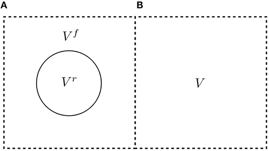
Figure 1. A particle in a confined system (A) in equilibrium with a bulk fluid phase (B).
The pressure of the rock particle depends on the volume of the particle. The relation of the two pressures is according to Hill
When this is combined with the equation right above, we find the relation we are after
which is the familiar Young-Laplace's law. By subtracting Equation (10) from Equation (8), we obtain an interesting new relation
The expression relates the integral and differential pressure for a spherical phase r of radius R. It is clear that this pressure difference is almost equally sensitive to the radius of curvature as is the pressure difference in Young-Laplace's law.
We see from this example how the integral pressure enters the description of small systems. The integral pressure is not equal to our normal bulk pressure, called the differential pressure by Hill, . While two differential pressures satisfy Young-Laplace's law in Equation (10), the integral pressures do not. The integral pressure has the property that when averaged over system A using Equation (4), it is the same as in system B, cf. Equation (6). This analysis shows that system A is a possible, or as we shall see proper, choice of a REV that contains the solid grain, while system B is a possible choice of a REV that contains only fluid.
The above explanation concerned a single spherical grain and was a first step in the development of a procedure to determine the pressure of a nano-porous medium. To create a more realistic model, we introduce now a lattice of spherical grains. The integral pressure of a REV containing n grains is given by an extension of Equation (3)
For each grain one may follow the same derivation for the integral and differential pressure as for the single grain. By using Equation (8), we obtain
where the last identity applies to spherical grains only. The differential pressure of the grains is given by a generalization of Equation (10)
where the last identity is only for spherical grains. The differential pressures again satisfy Young-Laplace's law at equilibrium.
When all grains are identical spheres and positioned on a fcc lattice, a properly chosen layer covering half the unit cell can be a proper choice of the REV. We shall see how this can be understood in more detail from the molecular dynamics simulations below. The REV is larger if the material is amorphous.
Cases I and II were simulated at equilibrium, while case II was simulated also away from equilibrium. Figures 3–8 illustrate the equilibrium simulations of the two cases.
The simulation box was three-dimensional with side lengths Lx, Ly, Lz.The box was elongated in the x-direction, Lx > Ly = Lz. Periodic boundary conditions were used in all directions in the equilibrium simulations. In the non-equilibrium simulation, reflecting particle boundaries [15] were applied to the x-direction, cf. section 3.5. Along the x-axis, the simulation box was divided into n rectangular cuboids (called layers) of size Δx, Ly, Lz, where Δx = Lx/n. The volume of each layer is Vl = ΔxLyLz. There are two regions A and B in the simulation box. Region A contains fluid (red particles) and grains (blue particles) and region B contains only fluid, see Figure 2. The regions, B = B1 + B2 and A do not have the same size, but the layers have the same thickness, Δx. The compressional energy of the fluid in one layer is, .
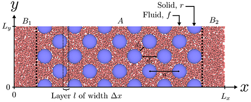
Figure 2. A slice of the simulation box in case II. The box has side lengths Lx, Ly, Lz, and properties are calculated along the x-axis in layers l of width Δx. Blue particles are grain r and red particles are fluid f. The A is the lattice constant of the fcc lattice, d1 and d2 are the two shortest surface-to-surface distances.
The simulation was carried out with LAMMPS [16] in the canonical ensemble using the Nosé-Hoover thermostat [17], at constant temperature T* = 2.0 (in Lennard-Jones units). The critical temperature for the Lennard-Jones/spline potential (LJ/s) is approximately . Fluid densities range from ρ* = 0.01 to ρ* = 0.7.
In case I the single spherical grain was placed in the center of the box. A periodic image of the spherical grain is a distance Lx, Ly and Lz away in the x, y and z-directions, see Figure 4A. The surface to surface distance of the spherical grains is d = Lα − 2R, where R is the radius of the grain, and α = y, z. In case I, each spherical grain has four nearest neighbors in the periodic lattice that is built when we use periodic boundary conditions. We considered two nearest neighbor distances; d = 4σ0 and d = 11σ0, where σ0 is the diameter of the fluid particles.
In case II, the spherical grains were placed in a fcc lattice with lattice constant a. The two shortest distances between the surfaces were characterized by and d2 = a − 2R, see Figure 2, where d1 < d2. We used d1 = 4.14σ0 and d1 = 11.21σ0, which is almost the same as the distances considered in case I. The corresponding other distances were d2 = 10σ0 and d2 = 20σ0. Each grain has 12 nearest neighbors at a distance d1.
In all cases we computed the volume of the grains , the surface area and the compressional energy of each layer, l, in the x-direction.
The particles interact with the Lennard-Jones/spline potential,
Each particle type has a hard-core diameter Rii and a soft-core diameter σii. There were two types of particles, small particles with σff = σ0, Rff = 0 and large particles with σrr = 10σ0, Rrr = 9σ0. The small particles are the fluid (f), and the large particles are the grain (r). The hard-core and soft-core diameters for fluid-grain pairs are given by the Lorentz mixing rule
We define the radius of the grain particles as R ≡ (σff + σrr)/2 = 5.5σ0, which is the distance from the grain center where the potential energy is zero. Fluid particles can occupy a position closer to the grain than this, this is illustrated in Figure 3. The figure shows the radial distribution function, g(r), of fluid particles around a single spherical grain. The density of fluid varied between ρ* = 0.1 and ρ* = 0.7. This shows that the average distance from the grain particle and the closest fluid particle is approximately 5.5σ0, but the fluid particles are able to occupy positions closer to the grain particle.
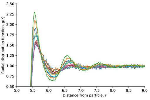
Figure 3. The radial distribution function of fluid particles around a grain, as shown in Figure 4. Results are shown for densities that vary between ρ* = 0.1 and ρ* = 0.7.
The interaction strength ϵij was set to ϵ0 for all particle-particle pairs. The potential and its derivative are continuous in r = rc,ij. The parameters aij, bij and rs,ij were determined so that the potential and the derivative of the potential (the force) are continuous at r = rs,ij.
The contribution of the fluid to the grand potential of layer l is [12]
where is the fluid differential pressure, the fluid volume, mi and vi are the mass and velocity of fluid particle i. The first two sums are over all fluid particles i in layer l, while the second sum is over all other particles j. Half of the virial contribution, the second term in Equation (17), is assigned to particle i and the other half to particle j. The virial contribution assigned to the solid particles are not included. rij ≡ ri − rj is the vector connecting particle i and j, and fij = −∂uij/∂rij is the force between them. The · means an inner product of the vectors. The computation gives , which is the contribution to the integral pressure in layer l from the fluid particles, accounting for their interaction with the grain particles.
We used the reflecting particle boundary method developed by Li et al. [15] to generate a pressure difference across the system along the x-axis. Particles moving from right to left pass the periodic boundary at x = 0 and x = Lx with probability (1 − αp) and reflected with probability αp, whereas particles moving from left to right pass freely through the boundary. A large αp gives a high pressure difference and a low αp gives a low pressure difference.
The results of the molecular dynamics simulations are shown in Figures 4–8 (equilibrium) and Figures 9, 10 (away from equilibrium). The porous medium structure was characterized by its pair correlation function, cf. Figure 3. The compressional energy was computed according to equation 4 in case I with a single spherical grain and case II with a lattice of spherical grains.
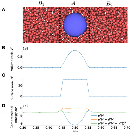
Figure 4. (A) Illustration of case I, a single spherical grain surrounded by a fluid phase with d = 4σ0. (B) Volume of grain, Vr, (C) surface area Ωfr and (D) compressional energy pV as a function of the x-axis of the simulation box.
We computed the compressional energy, plVl, in the bulk liquid (region B) and in the nano-porous medium (region A). In the bulk liquid we computed the pressure directly from the compressional energy, because (not shown).
Figures 4, 6 show the various contributions to the compressional energy, cf. equation 4. The grain particles were identical and the system was in equilibrium, so the integral pressure in the grains was everywhere the same, . Similarly, the surface tension was everywhere the same, .
The grain pressure and surface tension γfr were fitted such that the pressure is everywhere the same and are plotted as a function of the fluid pressure pf. The results for case II were next used in Figures 9, 10 to determine the pressure gradient across the sequence of REVs in the porous medium.
The single sphere case is illustrated in Figure 4A. Figures 4B,C show the variation in the volume of the porous medium (rock), , and the surface area between the rock and the fluid, Ωfr, along the x-axis of the simulation box. The two quantities were determined for all layers, l, and these results were used in the plots of Figures 4B,C. To be representative, the REV must include the solid sphere with boundaries left and right of the sphere. In order to obtain pREVVREV we summed plVl over all the layers in the REV. At equilibrium, pREV = p, where p is the pressure in the fluid in region B. For the REV we then have
where we used that and . We know the values of all the elements in this equation, except and γfr. The values of and γfr are fitted such that the pressure, p in Equation (18) is everywhere the same. With these fitted values available, we calculated plVl of each layer from
The contributions to the compressional energy in this equation for case I are shown in the bottom Figure 4D. We see the contribution from (1) the bulk fluid , (2) the bulk fluid and grain and (3) the total compressional energy, , which gives the pressure of the REV when summed and divided with the volume of the REV.
Figure 4D shows clearly that the bulk pressure energy gives the largest contribution, as one would expect. It is also clear that the surface energy is significant. As the surface to volume ratio increases, the bulk contributions may become smaller than the surface contribution (not shown). In the present case, this will happen when the radius of the sphere is 2.25σ0. For our grains with R = 5.5σ0, this does not happen.
The plots of and γfr as functions of p in region B are shown in Figure 5. The values for d = 4σ0 and d = 11σ0 are given in the same plots. We see that the plots fall on top of each other. This shows that the integral pressure and the surface tension are independent of the distance d in the interval considered. If confinement effects were essential, we would expect that and γfr were functions of the distance d between the surfaces of the spheres. When the value of d decreases below 4σ0, deviations may arise, for instance due to contributions from the disjoining pressure. Such a contribution is expected to vary with the surface area, and increase as the distance between interfaces become shorter. In plots like Figure 5, we may see this as a decrease in the surface tension.
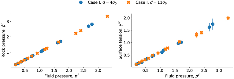
Figure 5. Fitted grain pressure and surface tension γfr as a function of pressure p for a sphere (characteristic length d = 4σ0 and d = 11σ0).
Consider next the lattice of spherical grains, illustrated in Figure 6A. Figures 6B,C give the variation in the volume of the porous medium and surface area, Ωfr, along the x-axis.
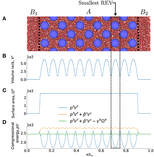
Figure 6. (A) Illustration of case II, a lattice spherical grain surrounded by a fluid phase with a = 20σ0. (B) Volume of grain, Vr, (C) surface area Ωfr and (D) compressional energy pV as a function of the x-axis of the simulation box. The smallest REV is a unit cell.
When the REV in region A is properly chosen, we know that pREV = p. In equilibrium, the pressure of the REV is constant in the bulk liquid phases, in regions B1 or B2, where p is the pressure of the fluid in region B. In order to obtain pVREV in region A, we sum plVl over all the layers that make up the REV, and obtain
To proceed, we find first the values of all the elements in this equation, except and γfr. The values of and γfr are fitted such that the pressure is everywhere the same. Using these fitted values, we next calculated of each layer using
The contributions to the compressional energy in this equation are shown in three stages in Figure 6D: (1) bulk fluid contribution , (2) bulk fluid and grain contribution and (3) the total compressional energy, . Figure 6D shows clearly that the bulk contribution is largest, as is expected. However, the surface energy is significant.
From Figure 6B it follows that a proper choice of the REV is a unit cell, because all REVs are then identical, (except the REVs at the boundaries). The integral over plVl in these REVs is the same and equal to pVREV. The layers l are smaller than the REV and as a consequence will vary, a variation that is seen in Figure 6D.
The values for and γfr are shown as a function of pf for case II in Figure 7 for d1 = 4.14σ0 and d1 = 11.21σ0. We see now a systematic difference between the values of and γfr in the two cases. The integral pressure and the surface tension increases as the distance between the grains decreases. The difference in one set can be estimated from the other. Say, for a difference in surface tension Δγfr we obtain for the same fluid pressure from equation 11, a difference in integral pressure of . This is nearly what we find by comparing the lines in Figure 6, the lines can be predicted from one another using R = 6.5σ0 while the value in Figure 3 is R = 5.5σ0. The difference may be due to the disjoining pressure. Its distribution is not spherically symmetric, which may explain the difference between 6.5σ0 and 5.5σ0.
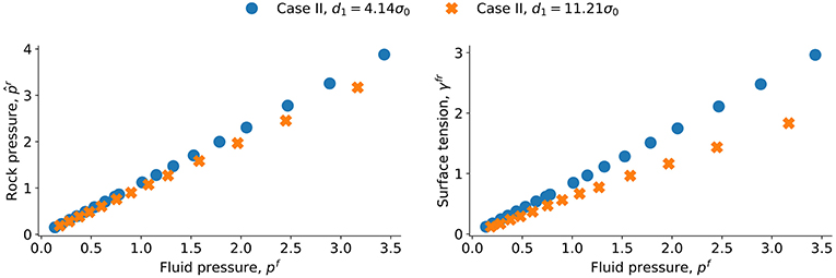
Figure 7. Fitted grain pressure and surface tension γfr as a function of pressure p for the lattice of spheres (characteristic length d1 = 4.14σ0 and d1 = 11.21σ0).
The results should be the same as for case I for the larger distance, and indeed that is found, cf. Figure 8. As the distance between the grain surfaces increases, we expect the dependence on confinement to disappear, and this is documented by Figure 8 where the two cases are shown with distances d = 11σ0 and d1 = 11.21σ0, respectively. The curves for the single grain and lattice of grains overlap.
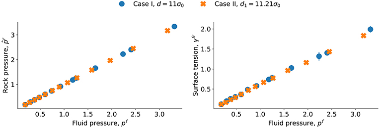
Figure 8. Fitted grain pressure and surface tension γfr as a function of pressure p for the sphere (characteristic length d = 11σ0) and a lattice of spheres (characteristic length d1 = 11.21σ0).
The knowledge gained above on the various pressures at equilibrium is needed to construct the REV. The size of the REV includes the complete range of potential interactions available in the system, but not more. To find a REV-property, we need to sample the whole space of possible interactions. The thickness of the REV is larger than the layer thickness used in the simulations.
Our analysis therefore shows that the pressure inside grains in a fcc lattice and the surface tension, depends in particular on the distances between the surfaces of the spheres, including on their periodic replicas. A procedure has been developed to find the pressure of a REV, from information of the (equilibrium) values of and γfr as a function of pf. It has been documented in particular for nano-porous medium, but is likely to hold for other lattices, even amorphous materials when the REV can be defined properly.
Figure 9 illustrates the system in the pressure gradient, where Figure 9B shows the compressional energy, pV, along the x-axis. The dip in the pressure close to x = 0 is caused by the reflecting particle boundary, cf. section 3.5. The reflecting particle boundary introduces a surface between the high pressure on the left side and the low pressure on the right side.
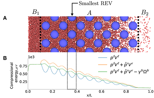
Figure 9. (A) Illustration of case II in a pressure gradient. (B) Compressional energy pV variation across the system.
To show first how a REV-property is determined from the layer-property, consider again the compressional energies of each layer. In the analysis we used the fcc lattice with lattice parameter a = 20σ0. The volume of the grain, Vr, and the surface area, Ωfr, varied of course in the exact same way as in Figures 6B,C. The pressure gradient was generated as explained in section 3.5. The pressure difference between the external reservoirs B1 and B2 was large, giving a gradient with order of magnitude 1012 bar/m. The fluid on the left side is liquid-like, while the fluid on the right side is gas-like. The smallest REV as obtained in the analysis at equilibrium is indicated in the figure.
In order to compute a REV variable away from equilibrium, we therefore follow the procedure described by Kjelstrup et al. [10] and choose a layer as a reference point. We then compute the average using five layers, two to the left, two to the right and the central layer. Moving one layer down the gradient, we repeat the procedure, and in this manner we obtain the property variation on the REV scale. The results of the simulation gave, for each individual layer, , as plotted in Figure 9B. The profile created by the REV-centers is shown in Figure 10. We see a smooth linear profile (central curve) as one would expect from the boundary conditions that are imposed on the system. Some traces of oscillation are still left in the separate contributions to the total compressional energy.
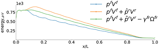
Figure 10. Compressional energy pV variation across the system smoothed over the representary elementary volume.
We have seen that a nano-porous medium is characterized by pressures in the fluid and the solid phases, as well as the surface tension between the fluid and the solid. When one reduces the size of a thermodynamic system to the nano-meter size, the pressures and the surface tensions become dependent on the size of the system. An important observation is then that there are two relevant pressures rather than one. Hill [1] called them the integral and the differential pressure, respectively. It is maybe surprising that the simple virial expression works so well for all pressure calculations in a fluid, but we have found that it can be used. We will next be able to study transport processes, where the external pressure difference is a driving force. The method, to compute the mechanical force intrinsic to the porous medium, may open interesting new possibilities to study the effects that are characteristic for porous media.
In a macro-scale description, the so-called representative elementary volume (REV) is essential. The REV makes it possible to obtain thermodynamic variables on this scale. We have here discussed how the fact that the macro-scale pressure is constant in equilibrium makes it possible to obtain the integral pressure in the solid, as well as the surface tension, of the liquid-solid contacts in the REV. An observation which confirms the soundness of the procedure is that we recover Young-Laplace's law for the differential pressures. The existence of a REV for systems on the nano-scale supports the idea of a REV that can be defined for pores also of micrometer dimension [10]. There is no conflict between the levels of description as they merge in the thermodynamic limit. The REV, as defined in the present work, may allow us to develop a non-equilibrium thermodynamic theory for the nano-scale.
The following conclusions can be drawn from the above studies
• We have obtained the first support for a new way to compute the pressure in a nano-porous medium. The integral pressure of the medium is defined by the grand potential. The definition applies to the thermodynamic limit, as well as to systems which are small, according to the definition of Hill [1].
• It follows that nano-porous media need two pressures in their description, the integral and the differential pressure. This is new knowledge in the context of nano-porous media.
• For a spherical rock particle of radius R, we derive a relation between the integral and the differential pressure in terms of the surface tension, . Their difference is non-negligible in the cases where Young-Laplace's law applies.
• We have constructed two models of a porous medium, case I with a single spherical grain and case II with a fcc lattice of spherical grains. The new method to compute the pressure in these nano-porous mediums is not specific to these two cases, it is general. The method can be used on, e.g., a random distribution of spherical grains, but the REV will need to be larger in order to include all possible microstates. The REV needs in general to be larger as the heterogeneity of the porous medium increases.
• To illustrate the concepts, we have constructed a system with a single fluid. The rock pressure and the surface tension are constant throughout the porous medium at equilibrium. The assumptions were confirmed for a porosity change from ϕ = 0.74 to 0.92, for a REV with minimum size of a unit cell.
• From the assumption of local equilibrium, we can find the pressure internal to a REV of the porous medium, under non-equilibrium conditions, and a continuous variation in the pressure on a macro-scale.
To obtain these conclusions, we have used molecular dynamics simulations of a single spherical grain in a pore and then for face-centered lattice of spherical grains in a pore. This tool is irreplaceable in its ability to test assumptions made in the theory. The simulations were used here to compute the integral rock pressure and the surface tension, as well as the pressure of the representative volume, and through this to develop a procedure for porous media pressure calculations.
Only one fluid has been studied here. The situation is expected to be more complicated with two-phase flow and an amorphous medium. Nevertheless, we believe that this first step has given useful information for the work to follow. We shall continue to use the grand potential for the more complicated cases, in work toward a non-equilibrium thermodynamic theory for the nano-scale.
All authors contributed equally to the work done. OG carried out the simulations.
The authors declare that the research was conducted in the absence of any commercial or financial relationships that could be construed as a potential conflict of interest.
The calculation power was granted by The Norwegian Metacenter of Computational Science (NOTUR). We thank the Research Council of Norway through its Centres of Excellence funding scheme, project number 262644, PoreLab.
1. ^ Another valid characteristic size is the size of the pores between the grains, but this follows from the two we have chosen.
2. Gray WG, Miller CT. Thermodynamically constrained averaging theory approach for modeling flow and transport phenomena in porous medium systems: 8. Interface and common curve dynamics. Adv Water Resour. (2010) 33:1427–43. doi: 10.1016/j.advwatres.2010.07.002
3. Bennethum LS, Weinstein T. Three pressures in porous media. Transp Porous Media. (2004) 54:1–34. doi: 10.1023/A:1025701922798
4. Magda J, Tirrell M, Davis H. Molecular dynamics of narrow, liquid-filled pores. J Chem Phys. (1985) 83:1888–901. doi: 10.1063/1.449375
5. Todd B, Evans DJ, Daivis PJ. Pressure tensor for inhomogeneous fluids. Phys Rev E. (1995) 52:1627. doi: 10.1103/PhysRevE.52.1627
6. Ikeshoji T, Hafskjold B, Furuholt H. Molecular-level calculation scheme for pressure in inhomogeneous systems of flat and spherical layers. Mol Simulat. (2003) 29:101–9. doi: 10.1080/102866202100002518a
7. Hafskjold B, Ikeshoji T. Microscopic pressure tensor for hard-sphere fluids. Phys Rev E. (2002) 66:1–4. doi: 10.1103/PhysRevE.66.011203
8. Hassanizadeh SM, Gray WG. Mechanics and thermodynamics of multiphase flow in porous media including interphase boundaries. Adv Water Resour. (1990) 13:169–86. doi: 10.1016/0309-1708(90)90040-B
9. Gray WG, Hassanizadeh SM. Macroscale continuum mechanics for multiphase porous-media flow including phases, interfaces. Adv Water Resour. (1998) 21:261–81. doi: 10.1016/S0309-1708(96)00063-2
10. Kjelstrup S, Bedeaux D, Hansen A, Hafskjold B, Galteland O. Non-isothermal transport of multi-phase fluids in porous media. the entropy production. Front Phys. (2018) 6:126. doi: 10.3389/fphy.2018.00126
11. Kjelstrup S, Bedeaux D, Hansen A, Hafskjold B, Galteland O. Non-isothermal transport of multi-phase fluids in porous media. Constitutive Equations. Front Phys. (2019) 6:150. doi: 10.3389/fphy.2018.00150
12. Irving JH, Kirkwood JG. The statistical mechanical theory of transport processes. IV. The equations of hydrodynamics. J Chem Phys. (1950) 18:817–29. doi: 10.1063/1.1747782
13. Tolman RC. The effect of droplet size on surface tension. J Chem Phys. (1949) 17:333–7. doi: 10.1063/1.1747247
14. Helfrich W. Elastic properties of lipid bilayers: theory and possible experiments. Zeitschrift für Naturforschung C. (1973) 28:693–703.
15. Li J, Liao D, Yip S. Coupling continuum to molecular-dynamics simulation: reflecting particle method and the field estimator. Phys Rev E. (1998) 57:7259–67. doi: 10.1103/PhysRevE.57.7259
16. Plimpton S. Fast parallel algorithms for short - range molecular dynamics. J Comput Phys. (1995) 117:1–19. doi: 10.1006/jcph.1995.1039
Keywords: nano-porous media, thermodynamics of small systems, representative elementary volume, single phase fluid, molecular dynamics simulations
Citation: Galteland O, Bedeaux D, Hafskjold B and Kjelstrup S (2019) Pressures Inside a Nano-Porous Medium. The Case of a Single Phase Fluid. Front. Phys. 7:60. doi: 10.3389/fphy.2019.00060
Received: 30 January 2019; Accepted: 29 March 2019;
Published: 24 April 2019.
Edited by:
Daniel Bonamy, Commissariat á l'Energie Atomique et aux Energies Alternatives (CEA), FranceReviewed by:
Alberto Rosso, Centre National de la Recherche Scientifique (CNRS), FranceCopyright © 2019 Galteland, Bedeaux, Hafskjold and Kjelstrup. This is an open-access article distributed under the terms of the Creative Commons Attribution License (CC BY). The use, distribution or reproduction in other forums is permitted, provided the original author(s) and the copyright owner(s) are credited and that the original publication in this journal is cited, in accordance with accepted academic practice. No use, distribution or reproduction is permitted which does not comply with these terms.
*Correspondence: Olav Galteland, b2xhdi5nYWx0ZWxhbmRAbnRudS5ubw==
Disclaimer: All claims expressed in this article are solely those of the authors and do not necessarily represent those of their affiliated organizations, or those of the publisher, the editors and the reviewers. Any product that may be evaluated in this article or claim that may be made by its manufacturer is not guaranteed or endorsed by the publisher.
Research integrity at Frontiers
Learn more about the work of our research integrity team to safeguard the quality of each article we publish.