 Bjørn Skjetne
 Alex Hansen
- Porelab, Department of Physics, Norwegian University of Science and Technology, Trondheim, Norway
We study the effects realistic fracture criteria have on crack morphology obtained in numerical simulations with a stochastic discrete element method. Results are obtained with two criteria which are consistent with the theory of elasticity and compared with previous results using the original criterion, chosen when the method was first published. The conventional choice has been to consider the combined loading as an interaction between bending and tensile forces only, leaving out shear forces altogether. Moreover the combination of bending and tension used in the old criterion is correct only for plastic deformations. Our results show that the inclusion of shear forces have a profound effect on crack morphology. We consider two types of external loading, torsion applied to a circular cylinder and tension applied to a cube. In the tensile case, the exponent which characterizes scaling of crack roughness with system size is found to be very close to the experimental value ζ ~ 0.5 when realistic fracture criteria are used. In the present calculations we obtain ζ = 0.52, a value which remains constant for all disorders. It is proposed that the small-scale exponent ζ = 0.8 appears as a consequence of cleavage between crystal planes and consequently requires a different fracture criterion than that which is used on larger scales.
1. Introduction
Material properties have long been studied by regarding the material as a continuum, such as in finite element analysis. Many real materials, however, cannot be adequately described as a continuum. Examples are granular, fibrous or porous materials where multiscale discontinuous features have a profound influence on the fracturing behavior. Concrete is a typical and commonly occurring example [1, 2]. Such features cannot be included in a satisfactory way in a continuum model [3]. An alternative approach was introduced four decades ago, the distinct element method [4], which is particularly well suited to describe granular media [5]. This simulated the mechanical behavior of unbonded disks and spheres of variable sizes, the equations of motion being deduced from Newton's second law with elements interacting directly via contact forces. Although this system behaves like a granular material without cohesion, bonding was later introduced betwee the elements [6] and the elements themselves have also been generalized to deformable polyhedral blocks [7].
Another development took place within the statistical physics community, where the study of complex problems [8] gave rise to other approaches such as the central-force elastic spring model [9], the random fuse model [10], and the elastic beam lattice [11, 12]. Our model is based on the latter approach, where a macroscopic material is though to be made up of discrete elements arranged on a lattice or grid. Into this discretized version of the material random variations in structural properties are introduced at the scale of the discrete elements. This can be done for the elastic properties of the elements or, as is more common, such variations can be made to affect the individual breaking strengths of the elements. The resulting breakdown process, whether it takes the form of electrical failure in a network of fuses or elastic breaking of a discretized continuum, is complex and results in a rough interface [8].
Consequently crack morphology as quantified by the roughness exponent [13, 14] has been the focus of several studies. It can be measured experimentally [15–24] and is therefore an important quantity to be reproduced by theoretical models. The typically rough crack surface that is obtained in materials with a heterogeneous microstructure is due to a complex interplay between stresses and local variations in material structure. Variations can be due to a granular structure with different grain sizes, with grains being randomly distributed and subject to different bonding strengths, or it can be due to an underlying fibrous structure. Structural heterogeneity can also be due to pores and voids, or the presence of microscopic cracks, inclusions and fault lines. Strength variations can therefore manifest themselves in the form of weak spots or strong spots.
Fracturing in such media is a coupled process whereby stresses evolve according to how cracks grow while cracks develop according to how stresses are distributed. At some point the fracture process goes from being disorder dominated, where new cracks appear randomly, to being stress dominated, where smaller cracks merge into a large crack. A path is now forged through the medium by the moving crack front. In this scenario, the fracture criterion plays a decisive role in determining the exact nature of the path taken. In other words, its role is to decide the outcome of the interplay between stress and disorder. It is therefore extremely important to study how different fracture criteria influence the fracturing process. As we shall see the role played by the fracture criterion is also affected by, and intimately associated with, lattice morphology. A criterion which does not allow for failure in transverse loading will display a tendency toward fracturing along lattice planes.
In simple stochastic models of fracture, such as the random fuse model, there is not much choice as far as the fracture criterion is concerned. Here the ratio of the current which flows through an element to the burn-out threshold of that element is what constitutes the breaking criterion. There really is no other choice. In elastic fracture, on the other hand, there are several modes of loading and each of these can contribute to the breaking of an element. This is especially so whenever forces are defined in terms of “beams.” In the case of “springs” only axial forces exist on the scale of the individual element. When the full elastic response is included, however, an element breaks if the axial load exceeds a certain limit or if the shear exceeds a certain limit. In general the situation is a combined loading.
Griffith's analysis of cracks in brittle materials is by many considered to be the beginning of the field of fracture mechanics [25]. Griffith was motivated by Inglis' previous work which indicated that stresses should approach infinity in the vicinity of a sharp crack tip, causing brittle materials to fail catastrophically upon the slightest application of an external load [26]. Moreover, this result was independent of crack size and thus contradictory to the observation that large cracks propagate far more readily than short cracks. For the case of an infinite plate under uniaxial tension Griffith computed the strain energy release as a function of crack length and added this to the energy absorbed by the newly created crack surfaces. The first of these terms subtracts from the total strain energy and is thus negative, decreasing with the square of the crack length. The second term is positive since potential energy relevant to the breaking of atomic bonds increases, in this case linearly. For short crack lengths the positive linear term thus dominates, and stress has to be increased for the crack to grow. At a certain critical value of crack length, however, the quadratic dependency of the strain energy release rate becomes dominating and consequently crack growth becomes self-sustaining as the system seeks to globally minimize its total energy. Crack growth can now only be arrested by lowering the externally applied stress.
After initially computing the potential energy in an uncracked specimen, Griffith's approach was to fix the boundary to ensure that the external load did no work, before introducing a small crack. In our calculations the system is also subjected to displacement control, whereupon fracture proceeds according to where the system is most stressed. However, none of the fracture criteria used by us in our discrete element method contains a mechanism whereby cracks initially grow in a stable manner before going unstable. Without the presence of disorder our cracks grow in an unstable manner from the very beginning. Griffith's critical crack length in our model corresponds to the lattice constant.
We do not believe this represents a serious discrepancy with regard to Griffith's theory, except perhaps should we apply the model on very small scales. As we will conclude from our calculations, it is the large scale roughness exponent that is reproduced in discrete element modeling, provided the correct meso-scopic fracture criterion is used. The roughness exponent appearing at very small scales is probably characteristic of cleavage between crystal planes, due to the plateau-like morphology which (as we shall see) obtains in tensile-dominant fracturing. Whether or not such a mechanism should make any difference with regard to fracture surface morphology is, in our opinion, a question that is more pertinent to these small scales.
On a very different level, much effort has been expended within engineering communities to obtain simplified, yet realistic, interaction formulae relevant to various loading conditions within a wide range of fields. Typically, the nature of these fracture criteria depend on the type of material used, the shape or cross section of the element involved, and the specific application concerned. They can be theoretically derived, empirically deduced from laboratory tests, obtained from numerical calculations, or they can be based on a combination of approaches. Some of this is published in technical reports which are not widely circulated outside their respective fields, but much is to be found within specialized engineering journals.
Some examples of where load interactions have been investigated are in the biomechanics of bone [27–29], anchor bolts in concrete [30, 31], cylindrical shells or plates within naval [32–35] or aeronautical [36–43] construction, aerospace engineering [44–47], strength of steel structures [48–54] including beam columns [55–60], capacity of structures under fire conditions [61–63], internally pressurized pipes [64, 65] or tubular members under hydrostatic pressure [66, 67] in marine structures, in the strength of brazed joints [68, 69], the capacity of wood structures [70–73] or plate girders for use in bridge constructions [74–76], and in the design of transmission shafts [77]. Also, official guidelines exist as to the recommended safe load combinations that should be heeded in engineering designs [78–81].
In our model an elastic “beam” element is liable to break whenever the stress exceeds a threshold value. This stress depends on the combination of loads which act on the element and the most natural way to quantify it is via some interaction formula analogous to those mentioned above. Here we might also hastily mention a different class of fracture criteria, beginning with that developed by Tsai and Wu [82] for anisotropic materials. These are more fundamental than interaction formulae, being scalar functions of two strength tensors. Such fracture criteria are typically applied in finite element analysis of composite materials.
Stochastic fracture models were developed within the statistical physics community and consequently much interest has been focused on the complex process of interaction between stress and disorder. This is probably one reason why failure criteria have received less attention than what would have been the case within the engineering community.
In section 2 we introduce our discrete element model, while in section 3 we briefly outline how scale-invariant disorder is included in the model. The main purpose of the paper is outlined in section 4, where we derive and discuss the fracture criteria to be used in the calculations. Here we consider the various combined loadings such as axial force and bending, torsion and shear, and axial force and shear. Finally we rationalize how, in the context of our model, axial force, shear, bending and torsion should be combined. This gives us two slightly different fracture criteria, which we in section 5 apply in calculations for the fracturing of a cube under uniaxial tension. The results are then compared with results obtained in previous calculations with the old criterion. Visually, the most profound difference is seen in cases of intermediate disorder strength. Here samples are seen to become more rough due to the inclusion of shear forces in the fracture criterion. At the same disorders crack surfaces obtained with the old criterion have a plateau-like appearance, dominated by flat sections. We argue that the old criterion, without being relevant as a small-scale fracture criterion but simply due to being overly tensile-dominant, emulates the separation of atomic bonds between crystal planes. Such separation is what characterizes brittle fracture on very small scales, and the roughness exponent obtained experimentally on small scales, ζ ~ 0.8, happens to be close to that obtained in our own previous results using the old fracture criterion. Only as the disorder is increased to an unrealistically strong level can we obtain a decrease in the roughness exponent with the old criterion (the flat sections disappear). In marked contrast to this, both the new fracture criteria are shown to produce a roughness exponent which agrees with the large-scale experimental result, ζ ~ 0.5. Moreover, this result remains constant for all the disorders included in the current study. In order to further illustrate differences between the old criterion and the new criteria we study in section 6 the fracturing of cylindrical shafts. Here it is shown that the overly tensile-dominant old criterion produces helical fracture surfaces that are somewhat steeper with respect to the torsional axis than the expected 45-degree angle. More importantly, the inclusion of shear in the new criteria enables an adjustment to be made in the relative strength of shear vs. tensile thresholds. Thus, for a material stronger in tension than in shear, the fracture surface is seen to be perpendicular to the torsional axis. As soon as the material becomes weaker in tension than in shear (as is typical of brittle materials), the inclination of the fracture surface quite rapidly adopts the expected 45-degree angle. Finally, in section 7 we summarize our results.
An Appendix has also been included to further illustrate how combined loadings interact. To this end, square cross-section macroscopic “real” beams have been constructed from the discrete lattice elements. Calculations here employ slightly more complicated equations than those used to obtain the results of sections 5 and 6, since the various loadings are best visualized when deformations are large. Although the equations involved are non-linear and thus computationally more expensive, we only calculate the resulting deformation of an intact structure here - due to an external combined loading - not the entire fracture surface.
2. Discrete Element Model
Before describing our model we brielfy address the terminology used, i.e., by “discrete element model” we do not mean the model that was introduced by Cundall et al. [4], nor any of the many refined bonded-particle models that it has spawned over the years. These models comprise what is commonly referred to as distinct or discrete element models. Presently we refer to our model also as a discrete element model. Outside of the bonded-particle approach there have been mainly two ways to model forces within discontinuous media, either in terms of “springs” [83, 84] or in terms of “beams” [11, 12]. The former approach is simpler and less requiring of computational resources since in this case bending and shear forces are absent in the individual element (the spring) [9]. The latter approach is computationally more demanding but is also more realistic since it better approximates the mechanical response of a real solid, i.e., each “beam” element transmits axial forces, bending moments, transverse shear and torsion to its adjoining neighbors.
Our model is a deformable lattice in the form of a regular cube with size L × L × L, where forces between nodes are defined as if they were connected by thick elastic beams [85, 86]. A coordinate system is placed on each node, and the enumeration of connecting “beams” follows an anti-clockwise scheme within the XY-plane, i.e., beginning with the beam which lies along the positive X-axis and ending with that which extends up along the positive Z-axis, see Figure 1.
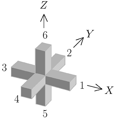
Figure 1. Enumeration scheme for the discrete “beam” elements of a cube lattice connecting node i to its nearest neighbors j = 1 to j = 6, showing the coordinate system with node i as its origin. Although cross-sections have been shown as square we do not intend to imply any specific geometry for the discrete elements.
At each stage of the breaking process, updated displacements for each node are obtained with the conjugate gradient method [87, 88]. The steps involved in the calculation correspond to Equations (40–46) in Batrouni and Hansen [89], replacing the kernel Dij in that paper by
where Xi … Wi are the components of force, to be outlined shortly. This approach minimizes the elastic energy by obtaining those displacements for which the sum of forces and moments on each node vanish, i.e., mechanical equilibrium. In Equation (1), xi, yi, and zi are the coordinate displacements of node i relative to its starting position before fracturing is initiated. Likewise, ui, vi, and wi are the angular displacements around the X-, Y-, and Z-axes, respectively (see Figure 1).
In the expressions for force and moment we have
where E and G are Young's modulus and the shear modulus, respectively, A is the area of the discrete element cross section, ℓ is its length and I the moment of inertia about the centroidal axis. Our choice of these parameters mirrors that of Herrmann et al. [12], i.e., the length is set to ℓ = 1 and we use α = 1, β = 30/7 and γ = 60/7. Additionally, we define the quantity
where J is the moment of inertia for torsion. Here we have arbitrarily chosen η = 1.
Since we do not currently wish to explore the parameter space relevant to different materials constants, we simply adopt the choice originally made for α, β and γ by Herrmann et al. [12], and later used by ourselves in Skjetne et al. [90], Skjetne et al. [91], and Skjetne et al. [92]. In the context of crack morphology, this has the advantage of enabling comparisons to be made between current and previous results that are solely based on differences in fracture criteria. As will be reiterated a few times throughout this paper, we do not wish the reader to think of the “beam” elements as entities with a given length-to-width ratio or with any specific cross-sectional shape. The “beam” is simply a concept whereby we define axial, flexural, torsional and shear forces between discretely chosen points within a continuous material. The current choice of parameters α, β, γ, and η in Equations (2) and (3) should, however, be thought of as representing “thick” beams.
In the following it will be convenient to define
for the relative displacements betweeen node i and its nearest neighbors, and similarly for the other five coordinates. Six terms contribute to each of the force components in Equation (1). For instance, if we imagined the neighboring nodes to be fixed, a translation xi of the central node i would induce axial forces in beams 1 and 3 and transverse forces in beams 2, 4, 5, and 6. If we take into account the displacements of the neighboring nodes as well, the axial force on node i from beam 1 is
while the transverse force on node i from beam 2, along the X-axis, is given by
In each case j refers to the neighbor depicted in Figure 1. Consequently,
is how the force on node i along the X-axis depends on the displacements and rotations of its six nearest neighboring nodes. Similar expressions are deduced for Yi or Zi by considering translations along the Y-axis or the Z-axis, respectively.
An angular displacement ui about the X-axis with the neighboring nodes fixed would create torque in beams 1 and 3, and bending in beams 2, 4, 5 and 6. More generally, the torque in node i from beam 1 is
while the bending moment from beam 2 is
For the angular force on node i about the X-axis and its dependence on the displacements of the six neighboring nodes, we have
now with similar expressions for Vi and Wi.
To express the thirty-six force components in Equation (1) more compactly,
and
are quantities which we define for notational convenience, to keep track of the signs and contributions from neighboring beams. The j in each case refers to the neighboring beams as shown in Figure 1. The Kronecker delta, moreover, has been used to construct
i.e., an operator which includes s and t in the sum over neighbors (excluding the other four), and
which instead excludes s and t from the sum over neighbors (including the other four).
For the six components making up the force on node i along the X-axis, i.e., Equation (7), we can now state this on a compact form as
and Yi as
In the same way, Zi becomes
Next, Equation (10) for angular displacements about the X-axis is written out in full as
and Vi, for angular displacements about the Y-axis, becomes
Lastly, for angular displacements about the Z-axis, we get
3. Disorder
To include structural disorder we generate a random number r on the unit interval [0, 1] and let this represent the cumulative threshold distribution. We assign thresholds according to , where D > 0 is a power law with a maximum threshold of 1 and a tail extending toward zero. The cumulative distribution function is then given by
where 0 ≤ tF ≤ 1. The case of D = 0 corresponds to all thresholds being the same (tF = 1), i.e., we have a homogeneous medium without structural disorder. An increase in the magnitude of the exponent |D| causes the coefficient of vari ation with respect to any two random numbers r and r′ on the interval [0, 1] to increase. Therefore large values of |D| correspond to strong disorders and small values to weak disorders.
Such a power-law distribution is a very simple and straightforward way to ensure that breaking thresholds are generated within a scale-invariant range [93–95]. Many other distributions are possible, but the main thing is that zero or infinity (or both) is included within the range of thresholds.
4. Fracture Criteria
The original fracture criterion introduced by Herrmann et al. [12] considers a combination of bending and axial force, where beams fail when
that is, using a squared term for the axial force and a linear term for the bending moment. The quantities tF and tM are thresholds for the amount of bending the element can support before failing. In applications other than stochastic modeling, there are two scenarios where this particular fracture criterion is frequently used. One is in connection with combined loadings for slender beams in compression [96]. The other is for materials where plastic yielding occurs, in which case the loading can be either tensile or compressive [97]. Presently we consider brittle fracture only.
4.1. Combined Axial Force and Bending
In wood constructions the region of safe loading for beam columns with rectangular cross sections, when subjected to a combination of axial tension and bending [81], is given as
in the unixial case, and
in the biaxial case, while the criterion for failure in compression is
in the uniaxial case, and
in the biaxial case. Deflection of the beam in the presence of a compressive force tends to magnify the moment that causes it, and consequently more emphasis is lent to the axial term. This distinction between tensile and compressive loading, however, is irrelevant to applications in the discrete element model. The reason is that the model is meant to describe a continuum rather than a physical lattice. In order to emulate the behavior of a continuum, elements defining forces between nodes should not be considered to be slender. In fact, they should not in any way buckle within the structure of the material! Interaction formulas relevant to compression should therefore have the same functional form as those relevant to tension.
This choice is easy to justify using standard elastic theory. In the two-dimensional case, we use the superposition principle for combined loadings. For a beam with its axis lying along the X-axis, and with a cross-section perpendicular to this, the normal stress caused by axial loading in the direction of the positive X-axis (tension) is given by
where P is the force and A is the cross-sectional area, see Figure 2A. Normal stresses also arise in bending. Assuming the beam is bent within the XZ-plane (upper surface tensile) these stresses are
where the bending moment is M and I is the moment of inertia of the cross-sectional area about the neutral axis. Normal stresses are seen to depend linearly upon the vertical distance z from the neutral axis, see Figure 2B. Adding Equations (27) and (28) we get
for the normal stress of the combined loading, that is,
and the maximum |σx| occurs along the top surface of the beam, as can be seen from Figure 2C. In contrast, below the neutral axis (negative z) the normal stress due to the axial load is reduced since Equation (28) becomes negative here. It is at its lowest along the bottom surface. If we reverse the sign on P and consider compressive axial forces, we find |σx| to be largest along the bottom surface for a beam bent like this.
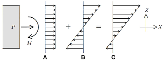
Figure 2. Superposition of stress in a beam subject to combined axial load P and bending moment M. The cross-sectional area is A, on which the stress distribution due to P alone is shown in (A), that due to M is shown in (B), and the superposition of the two is shown in (C).
A positive moment is defined as one where the beam is concave up, i.e., with the bottom surface in tension. Hence, with z = −c representing the outermost fiber on the cross section,
is the combined stress of axial tension and bending at this particular location. Dividing through Equation (31) by the maximum value of the normal stress within the elastic range, σp, we obtain
where
is the axial force at its elastic limit, and
is the bending moment at its elastic limit. Modeling a material which cannot deform plastically, i.e., which fails beyond the elastic limit, we can then identify Fy and My as breaking thresholds in F and M. If these thresholds are denoted tF and tM, one has to remove from the calculations those elements for which
and therefore, according to Equation (32), we must remove those elements for which the combination of F and M are such that
In our calculations we will not be interested in the details of where a “beam” is most stressed. What we require is to identify the maximum stress that occurs in a combined loading. In the case of axial tension Equation (23) selects those beams where the most stressed material fiber is beyond the breaking threshold (this will be on the convex side of the beam, be that on the upper or lower surface). In the case of compression, a beam in the same bent configuration would be most stressed on the opposite surface (the concave side), and this maximum stress is still given by Equation (23). We therefore need not distinguish between the convex and the concave sides in our application. In the discrete element model each element is either kept or removed depending on the magnitude of its greatest combined stress. The sign on F or M then becomes irrelevant.
For our purposes, then, elements that fail can be identified in three dimensions using
where the biaxial moment is given by
and the same thresholds tM apply in all planes of bending.
4.2. Combined Torsion and Shear
We next consider torsion combined with transverse shear. For generality and simplicity of illustration we regard circular cross-sections. As with bending and axial force, we use the superposition principle to obtain the stress distribution for the two loads combined. From the relationship between stress and strain, generalized Hooke's law, we have
We further assume for the stress distribution that
and for the shear strains that
where R is the maximum radius of the circular cross section and
is the radial distance from the center of the cross section. Hence stress and strain increase linearly toward the outer surface where the maximum value is attained for both. The relationship between applied torque T and shear stress on the cross section is
where J is the polar moment of inertia. We see from Equation (43) that the relationship between T and τ is analogous to the relationship between M and σ in Equation (28). For the average shear due to a vertical force we have
see Figure 3B. Combining Equations (43) and (44),
is the total shear force acting on the cross section. In Figure 3C the two quantities are seen to oppose each other on the extreme left, while they add up on the extreme right. Torque is taken to be positive as shown, i.e., when it is a vector in the positive X-direction.
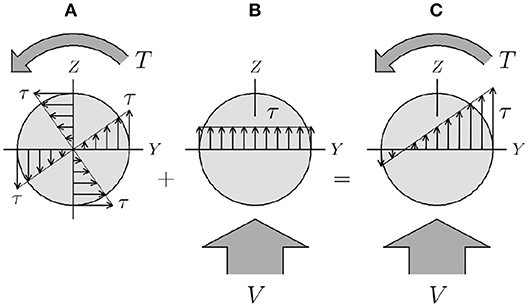
Figure 3. Distribution of shear stress on the cross section of a beam subjected to a transverse load V in the direction of the positive Z-axis and an anti-clockwise torque T about the X-axis. In (A) the radial distribution of stress due exclusively to torque is shown along the Y- and Z-axes, in (B) the uniform stress due to the vertical force V is shown along the Y-axis, and in (C) the superposition of those stresses on the Y-axis is shown.
As before, we are not concerned with where on any particular “beam” the stress is highest. Instead we simply identify the maximum stress that occurs with the aim to decide whether this is above or below the breaking threshold. If the element exceeds this threshold then it is removed as a carrier of force in the elastic equations. We see that Equation (45) is analogous to Equation (32) for combined bending and axial force. We therefore proceed by dividing through Equation (45) by the maximum allowable shear stress τy within the elastic range. We then obtain
where
is the maximum of the transverse force V in pure loading without a torque, and, from Equation (43),
is the maximum torque the element can sustain in pure rotational displacements. Assuming the element fails when
our criterion for failure under combined torque and shear becomes
Here we have defined tV = Vy and tT = Ty as breaking thresholds. Requiring only the maximum stress,
is our fracture criterion.
As for the breaking thresholds we use one threshold for each element in our calculations. Otherwise one might be led to make inferences about the detailed structure of each “beam,” i.e., such as where flaws are located. For instance, stress due to applied torque T is at its greatest furthest away from the axis of the element, see Equation (40), while shear stress due to a top-to-bottom vertical force V, according to Jourawski's formula, is at its greatest across the center of the section, midway between the top and bottom surfaces [98, 99]. Hence, whereas a flaw at the top or bottom surface will reduce the torque strength substantially, it will not to any great extent adversely affect the strength with which the element opposes vertical force. If one chooses to specify different thresholds for the two terms there are two obvious options. One is to assume a “realistic” distribution of thresholds whereby tV and tT are correlated so as to take into account different categories of flaws, the other is to simply assume that the thresholds are independently random for both types of loading. In our calculations we presently use the same threshold for both terms. This is based on the notion that “beam” elements are the basic building blocks in our system, i.e., they define the smallest length-scale. All heterogeneity pertaining to material flaws and/or variations in elastic properties are assumed to occur on scales at or above that of the individual discrete element.
4.3. Combined Axial Force and Shear
We regard a body element under biaxial stress, such as that shown in Figure 4. This body element is in a uniform state of stress. Stress being a second-order tensor, however, stress vectors vary according to the surface on which they act. In the following we regard a plane which intersects the body element at a given angle and observe how components vary as the angle is varied [100], see Figure 5. Here the X′Y′-coordinate system has been rotated through an angle α, such that the X′-axis coincides with the normal to the inclined plane. For a body element in equilibrium, the stress vector p acting on this plane is obtained by requiring the sum of forces to be zero. If we resolve the vector p in the XY-coordinate system, we obtain
the components of which are found to be
and
However, p can also be resolved in the X′Y′-coordinate system. Expressing first and in terms of px and py, as shown on the right in Figure 5, Equations (53) and (54) are next used to obtain , and in terms of σx, σy and τxy. We thus obtain
and
for the normal stresses, and
for the shear stress in the X′Y′-system. These are known as the transformation of stress equations [100], and allow us to determine the stress on any plane when the angle α and the stresses σx, σy, and τxy are known.
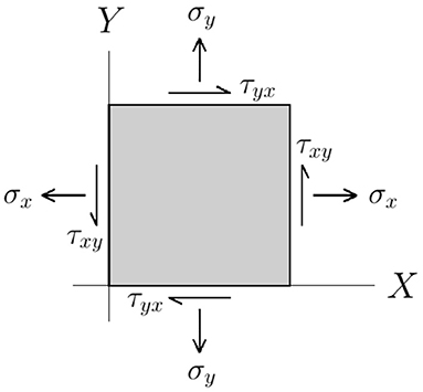
Figure 4. Elastic body element showing components of normal stress, σx and σy, and components of shear, τxy and τyx, on those surfaces that are parallel to the Z-axis.
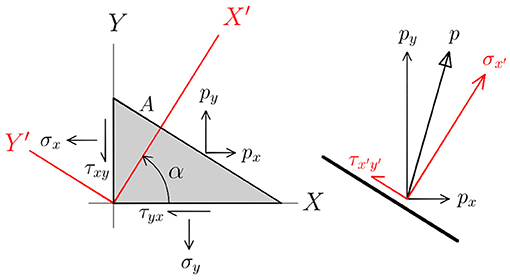
Figure 5. Free body with stress components on all surfaces. Decomposition of the stress vector p relative to the X′Y′-coordinate system is shown in red, decomposition relative to the XY-coordinate system is shown in black. The surface area of the inclined plane is A.
We next seek the extreme values of stress by varying the orientation of the inclined plane. Assuming structural integrity to be exceeded when the normal stress reaches a critical value, we evaluate
to obtain
This expression implies two solutions for α which are 90° apart. We also see that Equation (59) is identical to Equation (57), provided that . Extreme values of normal stress are therefore obtained where shear stress vanishes.
Substituting the angles which satisfy Equation (59) into Equation (55) we obtain, after a few manipulations,
for the maximum normal stress. “Beam” elements in our model are force carriers between lattice nodes, hence there is no normal stress perpendicular to the connecting line between these and Equation (60) becomes
where the maximum value of has been denoted σm. This expression is divided through by the failure threshold σf for the normal stress obtained in pure axial loading, to give
where we have introduced the dimensionless ratios of normal and shear stress to their respective failure thresholds,
as well as the parameter
for the ratio of the shear and normal failure stresses. This ratio, for steel, is often taken to be in the range 0.5−0.75. For rocks the ratio of tensile to shear strength corresponds to roughly k ~ 1, while compressive strength is at least ten times higher than tensile strength [101]. Assuming that our material fails when
our criterion for when a “beam” element fails is
where in Equation (62) loads and failure loads have been substituted for stresses and failure stresses.
Assuming instead that material integrity is exceeded when shear stress reaches a critical value,
is evaluated to obtain
the right-hand side of which is the negative reciprocal of Equation (59). This implies that the planes of maximum shear are at an angle of 45° with respect to the planes of maximum normal stress [100].
From Equation (68) expressions for cos2α and sin2α are obtained which are substituted into Equation (57). This gives
for the maximum shear stress. As with Equation (60) there is no normal stress perpendicular to the connecting line between nodes and
is obtained by setting σy = 0. Assuming the material fails for
where τf is the failure threshold for the shear stress, and dividing through Equation (70) by this quantity, we get
using the first of Equations (63), and Equation (64). The criterion for when a “beam” element should break is then
where in Equation (72) we have substituted loads and failure loads for stresses and failure stresses.
Plotting Equations (66) and (73) for different values of k it is seen that Equation (66) with k = 1 and Equation (73) with k = 0.5 provide interaction curves where the expressions
are both satisfied, see Figure 6. For values of k between 0.5 and 1 the failure envelope is a combination of Equations (66) and (73), corresponding to the innermost region bounded by the yellow and blue curves in Figure 6 (these have been shaded in gray). Equation (73) with k = 0.5, according to NASA TM X-73305 [44] and Steeve and Wingate [47], provides a convenient and conservative interaction curve when considering combined shear and axial loading, this is the shaded region enclosed entirely by the blue curve in the upper left pane of Figure 6. Hence, we choose
as our criterion. For k → 0.5 we see from Figure 6 that the shaded region approaches this criterion, while it approaches
when k → 1 (the yellow curve in the bottom right window). From Figure 6 it is also evident that Equation (75) is a good fit within the greater part of the range 0.5 < k < 1, deviating the most for values above k ≃ 0.9. For comparison, we will nonetheless also include results obtained with Equation (76) to see if this slightly more conservative alternative makes any difference.
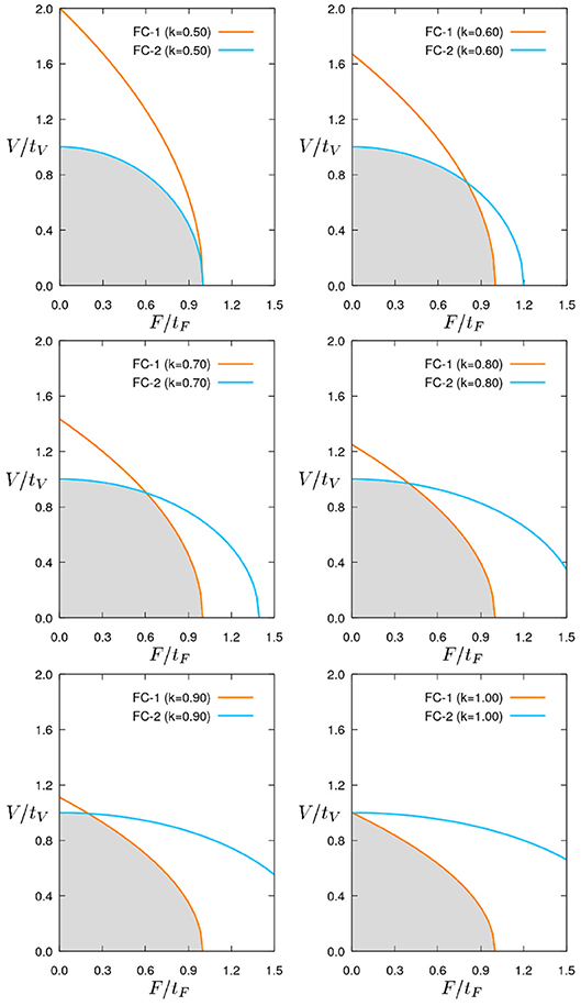
Figure 6. Failure envelopes corresponding of Equations (66) and (73), presently denoted FC-1 and FC-2, shown for k = 0.5, k = 0.6, k = 0.7, k = 0.8, k = 0.9 and k = 1.0. The gray-shaded regions correspond to load combinations for which “beam” elements do not break, i.e., safe loading regions.
4.4. Combined Axial Force, Shear, Torsion, and Bending
Finally we seek an interaction formula which combines axial force, shear, bending and torsion. The basic form of the fracture criterion is taken to be the interaction between axial force and shear, as given by Equation (75) or Equation (76). Within this prescription, bending is considered in combination with axial force, and torsion is considered as a contribution to shear.
With Equation (75) as our basic expression, the fracture criterion is then
where
is the total stress due to deformations which cause elongation, as shown in Figure 2, and
is the total stress from deformations contributing to shear, as shown in Figure 3. Note that in Equation (77) we have also assumed the same breaking threshold for loading in shear and tension, that is
In three dimensions the shear force V in Equation (79) acts within two perpendicular planes. If we consider beam 1 in Figure 1, extending along the positive X-axis, shear within the XZ- and XY-planes are combined into a bi-planar expression in Equation (79). Hence, we have
where VXY and VXZ are the respective contributions acting within the two planes. Likewise, in Equation (78) axial force F is combined with the largest of the moments at the ends of the “beam” element, i.e.,
where i is the near (node) end and j is the far (neighboring node) end of the “beam” element. If we again consider beam 1 in Figure 1 we now have
with My,i and Mz,i representing the contributions from bending obtained within the XZ- and XY-planes, respectively (My is the bending moment about the cross-sectional centroidal axis Y). The expression for Mj is similar.
Finally, for the sake of comparison, the k = 1 criterion based on maximum normal stress is also included. Hence, Equation (76) reads
where the quantities , and t are given by the same expressions as those in Equation (77) above.
Although a “beam” element, when regarded as a separate entity, can be strained, twisted and deformed in all manner of ways, we regard independent couplings between torsion and bending as less significant. Interaction between these two effects is still included, but only indirectly in the sense that bending contributes to axial stress, and torsion to shear, before the two are combined via Equations (75) or (76). This also applies to the combination of shear and bending, and to the combination of axial deformation and torsion – any direct interaction between these effects is assumed negligible. Indeed, it has been questioned whether a moment-shear interaction is at all relevant. Published results considering only these two deformation modes indicate a very weak interaction [102]. A curve with no interaction in Figure 6 would comprise two straight lines, describing a square where an upper-right vertex (1, 1) of the gray-shaded area would be the intersection of these lines. Basler [74], Sinur and Beg [75], and Sinur and Beg [76] display only a very weak “rounding” of this corner.
Also our assumption of a fracture criterion taking this form is not unreasonable considering that we intend to model a continuum, within which the “beam” is embedded and thereby considerably constrained by the surrounding medium. The situation would be different in considering an isolated beam which can move freely, and even more so if this beam is of the slender type or has a cross-sectional geometry that is important in the overall context. Moreover, in modeling a discretized continuum, realistic forces between nodes should preclude the use of discrete elements based on slender beams.
5. External Uniaxial Tension on a Cube
Using the model described in section 2, tensile fracture is initiated by imposing a uniform displacement vertically (along the Z-axis) on the top surface of the lattice. The edges of the cube are taken to be parallel with the coordinate axes. Discrete elements are removed one at a time, and at any stage in the fracturing process Equation (1) is used to calculate new displacements after a discrete element has been removed. The resulting distribution of stress, in conjunction with the breaking thresholds assigned, is used to identify which discrete element will break next. Exactly how this identification is made relies on the nature of the fracture criterion.
Fracture surfaces obtained for three different samples of size L = 32 are shown in Figure 7. The disorder used is one of intermediate strength, corresponding to D = 1 in the prescription outlined in section 3. For each sample the only difference between the one on the left and its counterpart on the right is the fracture criterion used. Samples on the left have been broken with the original fracture criterion, Equation(22), while Equation (77) has been used for those on the right. For the three samples shown the fracture surfaces appear roughly at the same position vertically on the lattice. Slopes, elevated areas and depressions sometimes also appear in the same locations. Although some samples appear superficially similar for the two fracture criteria, others again differ substantially. A closer look at the three samples in Figure 7, however, reveals an important difference between fracture surfaces obtained with these two criteria. This difference, moreover, pertains to all samples. Specifically, those obtained with Equation (77) display a pronounced roughness, in stark contrast with those obtained with Equation (22). In the latter case fracture surfaces are seen to consist of flat sections that are stepped up or down relative to each other – reminiscent of a landscape of “plateaus.” Fracture surfaces evidently look very different depending on which of the two criteria one uses.
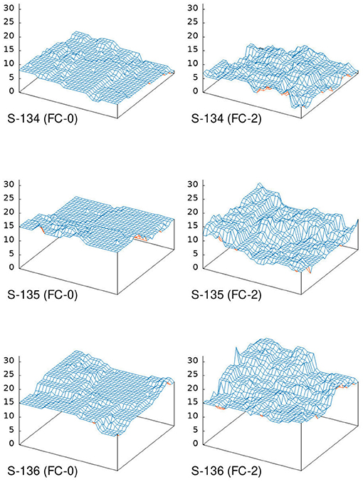
Figure 7. Comparison of fracture surfaces obtained with different fracture criteria. Three different samples are shown, S-134, S-135, and S-136. FC-0 denotes the “original” criterion, Equation (22), and FC-2 denotes the “maximum shear stress” criterion, Equation (77). Fracture interfaces are red on the underside and blue on top.
Such a difference in appearance could, however, also be obtained with the same fracture criterion by increasing or decreasing the magnitude of structural disorder [92]. The question is: does the morphology change in more fundamental ways than just to provide an offset in the roughness with respect to disorder strength? To answer this we turn to a standard yardstick in brittle fracture calculations, i.e., the exponent which characterizes how surface roughness scales with system size [8, 13, 15, 103]. Fracture surfaces have been found to be self-affine, meaning that if lengths within the fracture plane are scaled by a factor λ then lengths perpendicular to this plane scale by a factor λζ, where ζ is the roughness exponent. A self-affine relationship W ~ Lζ is therefore obtained, and this appears as a straight line in a log-log plot. Results have been obtained for ζ with various models, such as the random fuse model in 2D [104–106] and in 3D [107–110], and in 3D with networks of elastic springs [111]. Results have also been obtained with the beam lattice in 2D [90, 112]. The first result in 3D appeared in Skjetne et al. [113] and later in Skjetne et al. [92] and [114], with ζ varying according to the fracture criterion used, and possibly also with other parameters involved, such as strength of disorder and choice of materials constants.
Quantification of surface roughness is done in the same way as in Skjetne et al. [92], i.e., as the root-mean-square variance perpendicular to the fracture plane,
where zx(i) is the vertical height of the first intact node encountered when moving down toward the lower remaining part of the structure (shown in Figure 7).
Previous calculations made with the “original” criterion, Equation (22), indicates a roughness exponent ζ which varies considerably with the magnitude of the disorder [92], i.e., 0.59 < ζ < 0.78. Here smaller values ζ ~ 0.6 correspond to strong disorder, |D| ≥ 2, and larger values ζ ~ 0.8 to intermediate disorder, D = 1. These exponents are therefore somewhat high compared with the large-scale experimental result, ζ ≃ 0.5 [24, 115]. In Figure 8 we show the roughness exponent obtained with the “original” criterion Equation (22), using D = 1.5. Not surprisingly the result, ζ = 0.72, lies between the results obtained for D = 1 and D = 2 in Skjetne et al. [92], that is, it lies between ζ = 0.78 and ζ = 0.62. Using Equation (77), however, the value of the exponent reduces to the much lower value of ζ = 0.52, very close to the experimentally reported value for large length scales. This is notable in light of the fact that the original criterion is wrong insofar as it only applies to fracture with plastic deformations. Furthermore, the result obtained with Equation (84), ζ = 0.54, is similar to that obtained with Equation (77). Both results are shown in Figure 9. A comparison of fracture surfaces obtained with Equations (77) and (84) is shown in Figure 10. The surfaces are seen to be very similar in this case, close examination reveals only minor differences between the three samples. Evidently, the inclusion of shear forces in the fracture criterion fundamentally changes the detailed morphology of the crack surface.
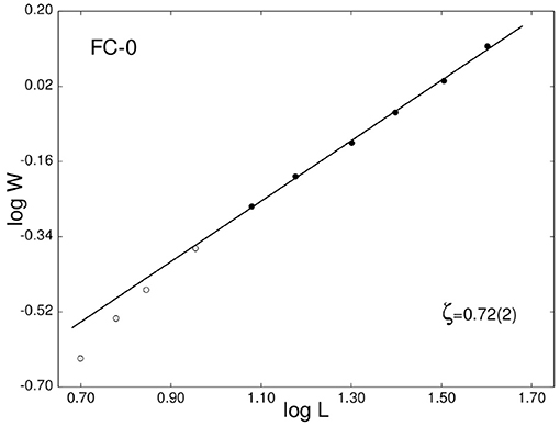
Figure 8. Log-log plot showing average roughness, W, as a function of system size, L, for a large number of fractured samples of each size. Disorder magnitude is D = 1.5. (FC-0) denotes the result obtained with the “original” fracture criterion, Equation (22). Black dots indicate those values to which the straight line has been fit using linear regression.
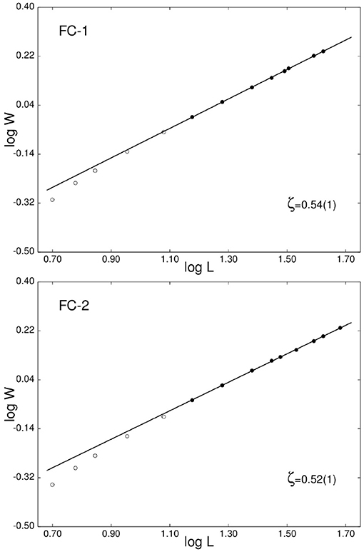
Figure 9. Log-log plots for average roughness, W, as a function of system size, L, for a large number of fractured samples. Disorder magnitude is D = 1.5. Shown at the top (FC-1) is the result obtained with the “maximum normal stress” criterion, Equation (84). Shown below (FC-2) is the result obtained with the “maximum shear stress” criterion, Equation (77). Black dots indicate those values to which the straight line has been fit using linear regression.
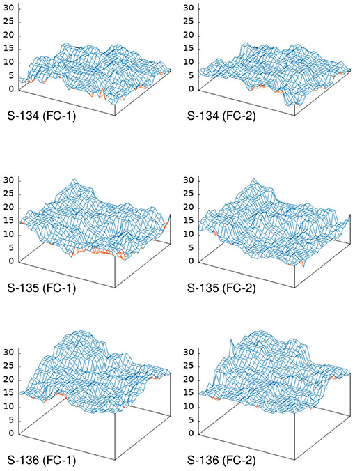
Figure 10. Comparison of fracture surfaces obtained with different fracture criteria. Three different samples are shown, S-134, S-135, and S-136. FC-1 denotes the “maximum normal stress” criterion, Equation (84), and FC-2 denotes the “maximum shear stress” criterion, Equation (77). Fracture interfaces are red on the underside and blue on top.
Brittle fracture on very small scales corresponds to the breaking of atomic bonds, thereby separating crystal planes. The resulting fracture surface is flat until the crack front encounters an obstacle, such as a grain boundary or a lattice defect. On small scales, therefore, it is not unreasonable to expect fracture surfaces akin to those shown on the left in Figure 7. These were obtained with the “erroneous” criterion, Equation (22), which, while lending much weight to axial force, has only weak contributions from bending and none from shear.
Equation (22) should, of course, not be regarded as an adequate criterion for brittle fracture on small scales. While the large scale fracture criteria, Equations (77) and (84), were derived from the theory of elasticity, a small scale criterion would require an analysis which takes into account the microscopic nature of the structure, such as, for instance, binding by interatomic potentials. From this a relevant functional form could be devised for a fracture criterion to be used in discrete element modeling at small scales. This should lend appropriate weight to the tensile breaking which gives rise to the cleavage process that takes place between crystal planes. At the same time it should include a less dominating mechanism (based on bending or shear or both) that emulates encounters with grain boundaries and other discontinuities within the crystal structure of the material.
This picture goes a long way toward explaining why two different exponents are obtained in the experiments. In numerical modeling with an appropriate fracture criterion which includes breaking due to shear, we obtain ζ ~ 0.5 on scales large enough for shear to play an important role. Contarary to this, ζ ~ 0.8 is expected on scales sufficiently small to be dominated by the crystal structure, as indicated by an “erroneous” criterion, such as Equation (22), which lends a disproportionally strong weight to tensile breaking.
In previous calculations with Equation (22) it was seen that the large scale roughness exponent ζ ~ 0.5 is approached from above when the disorder strength is considerably increased, resulting in ζ = 0.62 being obtained for D = 2 and ζ = 0.59 for D = 4 [92]. The latter case, however, represents a material structure with quite extreme variations in local strength properties, perhaps unrealistically so for most materials.
It is worth noting that, with the new criteria given by Equations (77) and (84), the roughness exponent remains in the vicinity of ζ = 0.5 for all disorders included in the present study. In other words, the roughness appears to be universal with respect to disorder strength, in contrast with what was found in Skjetne et al. [92]. With D = 2 the exponents obtained with Equations (77) and (84) are ζ = 0.54 and ζ = 0.53, respectively. The result is shown in Figure 11. At D = 3 we obtain ζ = 0.53 with both criteria, this is shown in Figure 12. Finally, at D = 4 we obtain ζ = 0.52 using Equation (84), in this case we did not take the trouble to run an extra set of simulations for Equation (77). The result is shown in Figure 13. The apparently constant value which, within the uncertainties of the straight-line fit, seems to fit all disorder strengths currently investigated with new fracture criteria is ζ = 0.53.
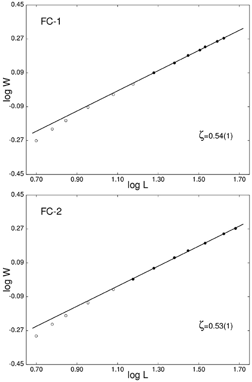
Figure 11. Log-log plots for average roughness, W, as a function of system size, L, for a large number of fractured samples. Disorder magnitude is D = 2. Shown at the top (FC-1) is the result obtained with the “maximum normal stress” criterion, Equation (84). Shown below (FC-2) is the result obtained with the “maximum shear stress” criterion, Equation (77). Black dots indicate those values to which the straight line has been fit using linear regression.
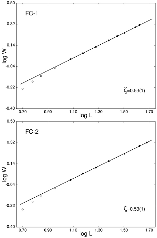
Figure 12. Log-log plots for average roughness, W, as a function of system size, L, for a large number of fractured samples. Disorder magnitude is D = 3. Shown at the top (FC-1) is the result obtained with the “maximum normal stress” criterion, Equation (84). Shown below (FC-2) is the result obtained with the “maximum shear stress” criterion, Equation (77). Black dots indicate those values to which the straight line has been fit using linear regression.
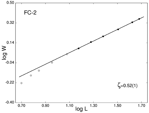
Figure 13. Log-log plot showing average roughness, W, as a function of system size, L, for a large number of fractured samples of each size. Disorder magnitude is D = 4 and FC-2 denotes the result obtained with the “original” fracture criterion, Equation (22). Black dots indicate those values to which the straight line has been fit using linear regression.
6. Externally Applied Torque on a Cylindrical Shaft
A typical property of brittle materials is that they are stronger in shear than in tension. As such, the criterion given by Equation (22) does capture one essential feature of brittle fracture, namely the preference toward failure in axially tensile loading. If this was the only requirement a fracture criterion even more simple than Equation (22) might have been sufficient, e.g., one that contains a single term only – the ratio of the axial load to the failure load.
In discrete element modeling there is, however, another feature which influences crack propagation and, ultimately, crack morphology: the geometry of the lattice discretization. Our current model is a cube lattice with nodes arranged as shown in Figure 1. For a crack to propagate obliquely with respect to the alignment of “beams,” breaks will have to occur by lateral (transverse) deformation as well as by longitudinal (axial) deformation. For a cube lattice strained in the Z-direction lateral breaks are those that occur within the XY-plane due to deformations transverse to the “beam” axis, i.e., shear deformations normal to (or bending deformations out of) this plane. In other words, a fracture plane which intersects the XZ-plane at an angle of exactly 45 degrees will require an equal number of transverse and longitudinal breaks. In localized fracture (very weak or no disorder) these two types of breaking events should alternate as the line of intersection between the crack front and the XZ-plane advances. For a fracture plane which advances at a steeper angle, the ratio of horizontal to vertical breaks increases, while a more shallow fracture plane likewise requires relatively fewer horizontal breaks.
Without providing for the possibility of shear failure, crack propagation would instead display a preference toward either the vertical or the horizonal plane, depending on the direction of the external loading. A situation requiring propagation along a plane inclined at 45 degrees is the fracture of a cylindrical shaft due to torque, see Figure 14. Directional inhomogeneity in the elastic properties of the cylinder (other than disorder) could modify the angle of the fracture surface, but in the case of a shaft with homogeneous material properties the emerging fracture angle should be 45 degrees in brittle fracture. Any deviation from this should instead be obtained by controlling the strength ratio of shear to tension in the thresholds. For a discrete element model such a freedom of choice is essential in order to obtain a crack which correctly reflects both the underlying structural disorder as well as other assumed material properties.
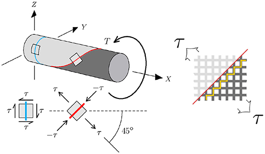
Figure 14. A positive valued torque T is applied on the right end of a cylindrical shaft, with the left end being held fixed. Shown in blue is an intersecting plane on which the shear stresses are at their highest. The associated material element is one of pure shear, with the largest values obtained vertically or horizontally. Shown in red is an intersecting helical surface perpendicular to which tensile forces are highest. The associated material element indicates the direction and value of the maximum tensile and compressive normal stresses. This element is contained within the lattice discretization on the right, with a numerical realization of the helical surface depicted in yellow.
We therefore next compare the new fracture criteria with the old criterion by considering torsional fracture in a cylindrical shaft. To construct such an object we first regard a rectangular column of discrete element “beams” using the cube lattice discretization. From this a cylindrical body is obtained by inscribing a circle within the limits of the square cross-section, before cutting away all discrete elements connected to nodes lying outside this circle. This is shown in Figure 15, for a structure subject to external torque. On the left the characteristic out-of-plane warping of non-circular cross sections is shown for a square cross-section in the XY-plane, while on the right a circular cross-section is shown. The amount of torsion involved is the same in both cases, and the vertical displacements have been exaggerated by a factor of fifty. Although it is unlikely that the warping of the square cross-section influences the nature of the fracture surface, we only consider circular cross-sections in the following. (The very minimal slanting seen at some of the edges of the circular cross-section on the right in Figure 15 are probably finite-size lattice effects).
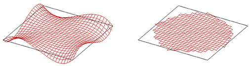
Figure 15. Mid-point sections in a body subject to torsion. On the left is a square cross-section, showing the characteristic out-of-plane warping obtained for non-circular cross-sections. On the right is a circular cross-section obtained by cutting elements outside a circle inscribed within the square. Vertical displacements have been magnified by a factor of 50.
Shear and bending stresses on the cross-section of a cylindrical shaft induced by torque is shown in Figure 16. At the top, (1) and (2) displays X6 and Y6, i.e., shear forces in the X- and Y-directions. These are obtained from the j = 6 components of Equations (15) and (16), respectively. Also shown, (3) is
i.e., the bi-planar shear of Equation (81). Below the shear stresses are shown bending stresses. These, (4) and (5), are V6 and U6, respectively. Also, (6) represents
or the biaxial bending moment of Equation (83). This combines bending within the XZ- and YZ-planes. Figure 16 shows that (with Equations (2) and (3) for the elastic constants) shear stresses are about twice as large as bending stresses. The necessity of using Equations (86) and (87), i.e., Equations (81) and (83), for consistency with rotational symmetry is also apparent.
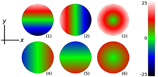
Figure 16. Stresses on the central cross-section of a cylinder subjected to an external torque. Shown are stresses in discrete element “beams” which connect horizontal layers in the cylinder, i.e., “beam” 6 in Figure 1. Shear stresses are displayed at the top and bending stresses at the bottom. See main text for more information.
Using the old criterion, Equation (22), a typical example of the helical fracture surfaces obtained is shown from five slightly different angles of rotation in Figure 17. The sample has been subjected to a counter-clockwise rotation at the top and a clockwise rotation at the bottom. All samples considered currently have weak disorder, i.e., using D = 0.4 in Equation (21). What is immediately apparent is that the angle of the fracture surface is rather steep. This is a reflection on the fact that Equation (22) is dominated by the axial term while having only a weak contribution from bending. It is this bending which provides the first local fractures since the main forces are due to displacements transverse to the vertical axis. At some point, however, breaking due to horizontal tension becomes important. Crack propagation in the form of separation along vertical lattice planes now becomes more dominant than breaking induced by bending within the horizontal plane. The resulting fracture surfaces tend to be very steep, significantly exceeding the 45 degree angle in Figure 14, as is evident in Figure 17.
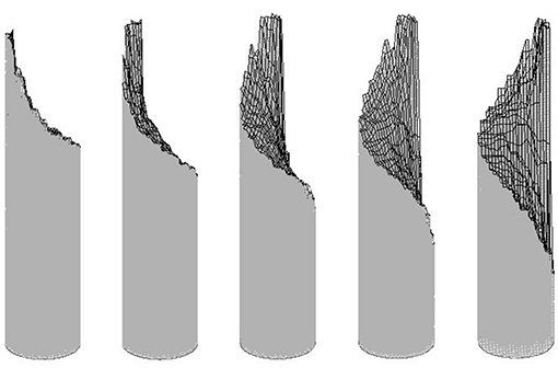
Figure 17. A cylindrical shaft with diameter d = 25 and height H = 201 which has been broken on the application of torque. The fracture criterion used is Equation (22). The shaft is shown from five slightly different angles.
If instead we use our new criterion, Equation (84), we have the option to vary the strength relationship between shear and tension. Assuming the material is stronger in tension than in shear we should expect “flat” fracture surfaces. Indeed, fracture surfaces obtained for a shear/tension ratio of 0.5 are quite flat and five samples are shown at top left in Figure 18. Such a strength ratio is typical of many metals, including steel [116]. These materials display less resistance toward the movement of dislocations within crystal planes and are thus more susceptible to failure due to shear deformations.
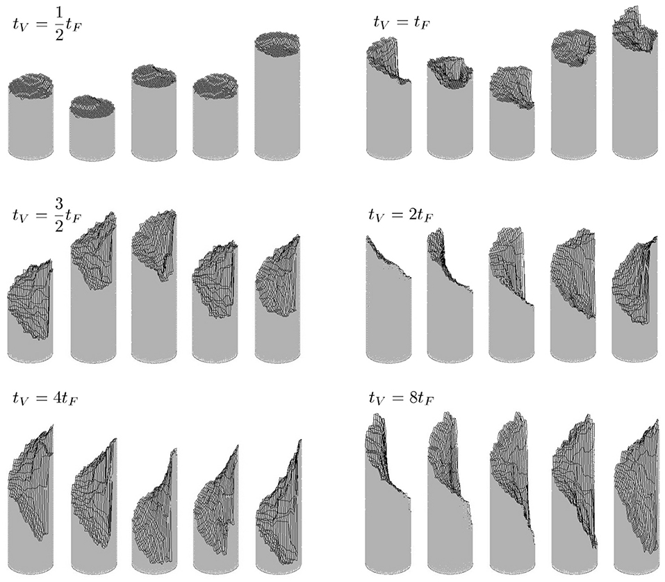
Figure 18. Cylindrical shafts with diameter d = 25 and height H = 101 broken by the application of torque, using different strength levels in the randomly generated breaking thresholds. The disorder used in all cases is D = 0.4, using Equation (21). At top left five different samples are shown having tensile thresholds twice as strong as those in shear. At top right tensile and shear thresholds are equal, also showing five different samples. At left in the middle row are shown five different samples with shear thresholds one and a half times as strong as the tensile thresholds, these samples have been rotated so as to display more or less the same view. At right in the middle row shear thresholds are twice as strong as tensile thresholds. A typical sample is shown from five slightly different angles in this case. At bottom left are shown five samples with shear thresholds four times stronger than tensile thresholds, these have been rotated to display more or less the same view. Finally, at bottom right a typical sample where shear thresholds are eight times stronger than tensile thresholds is included, this has been shown from five slightly different angles. In all cases the fracture criterion used is Equation (84).
Increasing the stochastically generated shear strength to the point where it equals the stochastically generated tensile strength changes the appearance of the fracture surfaces. Some of the samples now display a slanting surface while others are reminiscent of a cup-and-cone type surface (common in ductile fracture), see the five samples at top right in Figure 18.
Helical fracture surfaces of the type expected in Figure 14 appear as soon as the shear strength is increased beyond the tensile strength. For the five samples at mid left in Figure 18 shear is one and a half times stronger than tension. A single sample where shear is twice as strong as tension is shown from five slightly different angles at mid right in Figure 18. Strength ratios where shear is stronger than tension is typical of many rock types [117].
A further increase of shear strength relative to tensile strength causes the angle of fracture to become progressively steeper. At bottom left and bottom right in Figure 18 the ratios are four and eight, respectively.
Even when compared with these rather extreme cases, however, fracture surfaces obtained with the original criterion, Equation (22), are even more steep, as can be seen from Figure 17. In fact, they almost traverse the entire length of the sample. Such separation along vertical planes would perhaps be similar to the sort of fracture taking place when a broom stick is twisted until it breaks. Fracture then occurs as a separation of wood fibers parallel to the length axis of the shaft rather than as a breaking of such fibers in a direction normal to the length axis, as would be expected in shear fracture. This is especially the case in hardwoods, in softwoods fractures will also to some extent propagate across lengthwise fibers [118].
7. Concluding Remarks
The choice of fracture criterion is shown to have a profound effect on the crack morphology which obtains in calculations with a discrete element model for brittle fracture. The new fracture criteria are based on well known and long established relations and principles from the theory of elasticity, and replace a criterion which is really only relevant to plastic (rather than brittle) fracture. Modes of deformation such as axial strain, bending, shear and torsion are all included in the criteria used.
It is especially the inclusion of shear which most affects the results obtained. Visually, the most conspicuous change is observed at the weak end of the currently included range of disorders. Here the resulting fracture surfaces appear considerably more rough. The way this influences the self-affine properties of the crack is to lower the roughness exponent to a value consistent with experimental findings, i.e., ζ = 0.52. What is more, the roughness exponent remains at this value for all disorders currently included, indicating a universal value. An additional gain produced by allowing breaking in other deformation modes, notably shear, is to enable the crack front to move more freely with respect to the lattice topology. Otherwise, for a criterion with an axially dominant breaking mechanism, crack propagation will display a tendency to align itself in parallel with symmetry planes in the lattice. We have used a cube lattice, although this does not strictly reproduce the correct macroscopic response to an external loading. It is, however, less demanding on numerical resources than would be, say, an hexagonal close-packed lattice configuration.
A larger roughness exponent ζ ≈ 0.7 − 0.8 has been reported in experiments on small scale [14]. We do not see this in our numerical data. The existence of a small-scale larger roughness exponent and a large-scale smaller roughness exponent has also been reported in experiments on crack fronts constrained to move along two-dimensional planes [119]. Bouchaud et al. [120] suggested that the large roughness exponent on small scales would be due to damage coalescence on small scales. That is, the crack surface would merge with the cloud of damage surrounding it, thus roughening it. Gjerden et al. [121] demonstrated using the fiber bundle model [122] that this is indeed a mechanism for a crack front constrained to move along a two-dimensional plane. In this case, the damage cloud appears in front of the crack front, which then on small scales grows though it merging with the damage cloud. In three dimensions, the mechanism by which merger roughens the fracture surface would be different. We will follow up the present study by investigating whether this mechanism also is present in three-dimensional unconstrained crack growth.
Two new fracture criteria were included in this study, one based on maximum normal stress and the other on maximum shear stress. Both criteria give the same results for the roughness exponent and, based on the systems currently studied we could not see any difference in crack surface morphology, quantitatively or in visual appearance. A criterion which does not include shear breakage tends to promote the breaking of “beam” elements aligned in parallel with the direction of the applied load. Hence a majority of fracture surfaces perpendicular to the externally applied load are rendered flat. The inclusion of shear acts as a roughening mechanism in that breaking now also happens in elements that are perpendicular to the direction of the applied load and consequently the crack front can more readily move at an angle with respect to these flat regions. This means that the path taken by the crack, and thus its morphological properties, now more correctly reflects the underlying material inhomogeneities.
The sort of discrete element modeling that we have presented in this paper should be useful in many applications, for instance in modeling concrete structures or in biomechanics applications. We have included simple cylindrical structures in the current study but any cross-section can be easily made and the body of the structure in question can also be modified lengthwise to give a wide variety of shapes. Furthermore, the introduction of anisotropy in either strength or elastic properties is easily accomplished with such a model.
The current model does not include friction or contact after elements have been removed. We do not believe this seriously affects the results obtained for a system loaded in external tension or for breaking in torsion when elements are weaker in tension than in shear. Very large overhangs in a tensile situation would, of course, be broken away by friction forces but these overhangs are neglected anyway in the way we measure the roughness. This is done by looking straight down toward the surface and identifying the first intact element. For the disorder strengths included, even at the high end, we cannot see any overhangs in 3D, although such may be present in 2D where the effect of strong disorder tends to produce more sinuous crack lines. In 3D such 2D lines would be constrained by the neighboring lines to produce a less rough surface. Nevertheless, such effects are strong candidates for inclusion in future improvements of the model. In scenarios involving externally compressive loads, contact and friction are certainly important.
No investigation into how results depend on the chosen elastic constants has been made in this study, this should probably be addressed in a future study.
Author Contributions
All authors listed have made a substantial, direct and intellectual contribution to the work, and approved it for publication.
Funding
Research Council of Norway, project numbers 199970, 213462, and 262644.
Conflict of Interest Statement
The authors declare that the research was conducted in the absence of any commercial or financial relationships that could be construed as a potential conflict of interest.
Acknowledgments
This work was partly supported by the Research Council of Norway through its Centres of Excellence funding scheme, project number 262644.
Footnote
1. ^The discrepancy is mostly due to the fact that the small vertical shrinkage required in a pure bending in case “V” has not been taken into account. This would be necessary for the arc-length in the middle of the beam to equal the length of the beam in its relaxed state. The remaining discrepancy is due to the moment, being applied at the top and bottom ends, not being constant throughout the length of what is essentially a thick beam.
References
1. van Mier JGM. Concrete Fracture: A Multiscale Approach. Boca Raton, FL: Taylor & Francis Group (2013).
2. Lilliu G, van Mier JGM. 3D lattice type fracture model for concrete. Eng Fract Mech. (2003) 70:927–41. doi: 10.1016/S0013-7944(02)00158-3
3. Cundall PA. A discontinuous future for numerical modelling in geomechanics? Proc Inst Civ Eng Geotech Eng. (2001) 149:41–7. doi: 10.1680/geng.2001.149.1.41
4. Cundall PA, Strack ODL. A discrete numerical model for granular assemblies. Géotechnique. (1979) 29:47–65.
5. Pande GN, Beer G, Williams JR. Numerical Methods in Rock Mechanics. Chichester: John Wiley & Sons (1990).
6. Potyondy DO, Cundall PA. A bonded-particle model for rock. Int J Rock Mech Min Sci. (2004) 41:1329–64. doi: 10.1016/j.ijrmms.2004.09.011
7. Bobet A, Fakhimi A, Johnson S, Morris J, Tonon F, Yeung MR. Numerical models in discontinuous media: review of advances for rock mechanics applications. J Geotech Geoenviron Eng. (2009) 135:1547–61. doi: 10.1061/(ASCE)GT.1943-5606.0000133
8. Herrmann HJ, Roux S. Statistical Models for the Fracture of Disordered Media. Amsterdam: Elsevier (1990).
9. Feng S, Sen PN. Percolation on elastic networks: new exponent and threshold. Phys Rev Lett. (1984) 52:216–9. doi: 10.1103/PhysRevLett.52.216
10. de Arcangelis L, Redner S, Herrmann HJ. A random fuse model for breaking processes. J Phys Lett. (1985) 46:L585–90. doi: 10.1051/jphyslet:019850046013058500
11. Roux S, Guyon E. Mechanical percolation: a small beam lattice study. J Phys Lett. (1985) 46:L999–1004. doi: 10.1051/jphyslet:019850046021099900
12. Herrmann HJ, Hansen A, Roux S. Fracture of disordered, elastic lattices in two dimensions. Phys Rev B. (1989) 39:637–48. doi: 10.1103/PhysRevB.39.637
13. Bouchaud E. Scaling properties of cracks. J Phys Condens Matter. (1997) 9:4319–44. doi: 10.1088/0953-8984/9/21/002
14. Bonamy D, Bouchaud E. Failure of heterogeneous materials: a dynamic phase transition? Phys Rep. (2011) 498:1–44. doi: 10.1016/j.physrep.2010.07.006
15. Mandelbrot BB, Passoja DE, Paullay AJ. Fractal character of fracture surfaces of metals. Nature (London) (1984) 308:721–2. doi: 10.1038/308721a0
16. Måløy KJ, Hansen A, Hinrichsen EL, Roux S. Experimental measurements of the roughness of brittle cracks. Phys Rev Lett. (1992) 68:213–5. doi: 10.1103/PhysRevLett.68.213
17. Bouchaud E, Lapasset G, Planes J, Navèos S. Statistics of branched fracture surfaces. Phys Rev B. (1993) 48:2917–28. doi: 10.1103/PhysRevB.48.2917
18. Milman VY, Blumenfeld R, Stelmashenko NA, Ball RC. Experimental measurements of the roughness of brittle cracks-comment. Phys Rev Lett. (1993) 71:204. doi: 10.1103/PhysRevLett.71.204
19. Daguier P, Henaux S, Bouchaud E, Creuzet F. Quantitative analysis of a fracture surface by atomic force microscopy. Phys Rev E. (1996) 53:5637–42. doi: 10.1103/PhysRevE.53.5637
20. Daguier P, Nghiem B, Bouchaud E, Creuzet F. Pinning and depinning of crack fronts in heterogeneous materials. Phys Rev Lett. (1997) 78:1062–5. doi: 10.1103/PhysRevLett.78.1062
21. Ponson L, Bonamy D, Auradou H, Mourot G, Morel S, Bouchaud E. et al. Anisotropic self-affine properties of experimental fracture. Int J Frac. (2006) 140:27–37. doi: 10.1007/s10704-005-3059-z
22. Ponson L, Auradou H, Vié P, Hulin J-P. Low self-affine exponents of fractured glass ceramics surfaces. Phys Rev Lett. (2006) 97:125501. doi: 10.1103/PhysRevLett.97.125501
23. Ponson L. Crack propagation in disordered materials: how to decipher fracture surfaces. Ann Phys. (2007) 32:1–120. doi: 10.1051/anphys:2008044
24. Ponson L, Auradou H, Pessel M, Lazarus V, Hulin J-P. Failure mechanisms and surface roughness statistics of fractured fontainebleau sandstone. Phys Rev E. (2007) 76:036108. doi: 10.1103/PhysRevE.76.036108
25. Griffith AA. The phenomena of rupture and flow in solids. Phil Trans R Soc Lond. A. (1920) 221:163–98. doi: 10.1098/rsta.1921.0006
26. Inglis CE. Stresses in a plate due to the presence of cracks and sharp corners. Trans Inst Nav Archit. (1913) 55:219–41.
27. Crandall JR, Funk JR, Rudd RW, Tourret LJ. The tibia index: a step in the right direction. In: Kajzer J, Tanaka E, Yamada H, editors. Human Biomechanics and Injury Prevention Tokyo: Springer-Verlag (2000). p. 29–40.
28. Wang X, Guyette J, Liu X, Niebur GL. Axial-shear interaction effects on microdamage in bovine tibial trabecular bone. Eur J Morphol. (2005) 42:61–70. doi: 10.1080/09243860500095570
29. Ivarsson BJ, Genovese D, Crandall JR, Bolton JR, Untaroiu CD, Bose D. The tolerance of the femoral shaft in combined axial compression and bending loading. Stapp Car Crash J. (2009) 53:251–90. doi: 10.4271/2009-22-0010
30. McMackin PJ, Slutter RG, Fisher JW. Headed Steel anchor under combined loading. Eng J AISC. (1973) 10:43–52.
32. Ueda Y, Rashed SMH, Paik JK. Buckling and ultimate strength interaction in plates and stiffened panels under combined inplane biaxial and shearing forces. Mar Struct. (1995) 8:1–36. doi: 10.1016/0951-8339(95)90663-F
33. Guedes Soares C, Gordo JM. Compressive strength of rectangular plates under biaxial load and lateral pressure. Thin Wall Struct. (1996) 24:231–59. doi: 10.1016/0263-8231(95)00030-5
34. Cui W, Wang Y, Pedersen PT. Strength of ship plates under combined loading. Mar Struct. (2002) 15:75–97. doi: 10.1016/S0951-8339(01)00009-0
35. Cho S-R, Kim H-S, Doh H-M, Chon Y-K. Ultimate strength formulation for stiffened plates subjected to combined axial compression, transverse compression, shear force and lateral pressure loadings. Ships Offshore Struc. (2013) 8:628–37. doi: 10.1080/17445302.2013.810492
36. Lundquist EE, Stowell EZ. Strength Tests of Thin-Walled Elliptic Duralumin Cylinders in Pure Bending and in Combined Pure Bending and Torsion. Washington, DC: NACA Technical Note No.851 (1942).
37. Sherwood AW. The Strength of Thin-Walled Cylinders of D Cross Section in Combined Pure Bending and Torsion. Washington, DC: NACA Technical Note No.904 (1943).
38. Guggenheim Aeronautical Laboratory. Some Investigations of the General Instability of Stiffened Metal Cylinders, VII - Stiffened Metal Cylinders Subjected to Combined Bending and Torsion. Washington, DC: NACA Technical Note No.911 (1943).
39. Bruhn E. Tests on Thin-Walled Celluloid Cylinders to Determine the Interaction Curves under Combined Bending, Torsion, and Compression or Tension Loads. Washington,DC: NACA Technical Note No.951 (1945).
40. Batdorf SB, Stein M. Critical Combinations of Shear and Direct Stress for Simply Supported Rectangular Flat Plates. Washington, DC: NACA Technical Note No.1223 (1947).
41. Peters RW. Buckling Tests of Flat Rectangular Plates under Combined Shear and Longitudinal Compression. Washington, DC: NACA Technical Note No.1750 (1948).
42. Budiansky B, Stein M, Gilbert AC. Buckling of a Long Square Tube in Torsion and Compression. Washington, DC: NACA Technical Note No.1751 (1948).
43. Baker DJ, Fudge J, Ambur DR, Kassapoglou C. Optimal design and damage tolerance verification of an isogrid structure for helicopter application. In: 44th AIAA/ASME/ASCE/AHS Structures, Structural Dynamics, and Materials Conference, 7-10 April 2003, Norfolk, VA (2003).
44. NASA TM X-73305. Astronautic Structures Manual, Vol. I, Huntsville, AL: Marshall Space Flight Center (1975).
45. Flom Y. Failure Assessment Diagram for Brazed 304 Stainless Steel Joints, NASA/TM 2011-215876. Greenbelt, MD: Goddard Space Flight Center (2011).
46. Flom Y, Jones JS, Powell MM, Puckett DF. Failure Assessment Diagram for Titanium Brazed Joints, NASA/TM 2011-215882. Greenbelt, MD: Goddard Space Flight Center (2011).
47. Steeve BE, Wingate RJ. NASA/TM 2012-217454. Huntsville, AL: Marshall Space Flight Center (2012).
49. Neal BG. Effect of shear force on the fully plastic moment of an I-Beam. J Mech Eng Sci. (1961) 3:258–66. doi: 10.1243/JMES_JOUR_1961_003_033_02
50. Duan L, Chen WF. Design interaction-equation for steel beam-columns. J Struct Eng. (1989) 115:1225–43. doi: 10.1061/(ASCE)0733-9445(1989)115:5(1225)
51. Al-Chaar GK, Randolph DJ, Lamb GE, Desai PJ. ERDC/CERL TR-01-11, Structural Evaluation of Aircraft Hangar 46. Corpus Christi Army Depot, US Army Corps of Engineers, Engineer and Development Center (2001).
52. Sarawit AT, Peköz T. Cold-Formed Steel Frame and Beam-Column Design. American Iron and Steel Institute, Research Report RP03-2 (2003).
53. Karsan Demir PEI. Fixed offshore platform design. In: Chakrabarti SK editor. Handbook of Offshore Engineering, Vol. I, London: Elsevier Ltd., (2005).
54. Liu Y, Xu L, Grierson DE. Combined MVP failure for steel cross-sections. J Constr Steel Res. (2009) 65:116–24. doi: 10.1016/j.jcsr.2008.03.019
55. Neal BG. The effect of shear and normal forces on the fully plastic moment of a beam of rectangular cross section. J Appl Mech. (1961) 28:269–74. doi: 10.1115/1.3641666
56. Santathadaporn S, Chen WF. Interaction Curves for Sections under Combined Biaxial Bending and Axial Force. Fritz Engineering Laboratory Report No. 331.3, Lehigh University (1968).
57. Nie JG, Wang YH, Fan JS. Experimental research on concrete filled steel tube columns under combined compression-bending-torsion cyclic load. Thin Wall. Struct. (2013) 67:1–14. doi: 10.1016/j.tws.2013.01.013
58. Vasdravellis G, Uy B. Shear strength and moment-shear interaction in steel-concrete composite beams. J Struct Eng. (2014) 140:04014084. doi: 10.1061/(ASCE)ST.1943-541X.0001008
59. Bai Y, Jin W-L (editors). Buckling/collapse of columns and beam-columns. In: Marine Structural Design, 2nd ed., Oxford: Butterworth-Heinemann (2016). p. 19–37.
60. Chen S, Peng W, Yan W. Experimental study on steel reinforced concrete columns subjected to combined bending-torsion cyclic loading. Struct Des Tall Spec. (2018) 27:e1479. doi: 10.1002/tal.1479
61. Vila Real PMM, Lopes N, Simões da Silva L, Piloto P, Franssen J-M. Towards a consistent safety format of steel beam-columns: application of the new interaction formulae for ambient temperature to elevated temperatures. Steel Comp Struct. (2003) 3:383–401. doi: 10.12989/scs.2003.3.6.383
62. Vila Real PMM, Lopes N, Simões da Silva L, Piloto P, Franssen J-M. Numerical modelling of steel beam-columns in case of fire–comparisons with eurocode 3. Fire Safety J. (2009) 39:23. doi: 10.1016/j.firesaf.2003.07.002
63. Reis A, Lopes N, Real PV. Shear-bending interaction in steel plate girders subjected to elevated temperatures. Thin Wall Struct. (2016) 104:34–43. doi: 10.1016/j.tws.2016.03.005
64. Mohareb M. Plastic interaction relations for pipe sections. J Eng Mech. (2002) 128:112–20. doi: 10.1061/(ASCE)0733-9399(2002)128:1(112)
65. Bai Y, Bai Q. Residual strength of dented pipes with cracks. In: Subsea Pipelines and Risers. Oxford: Elsevier Ltd., (2005).
67. Bai Y, Jin W-L. Ultimate strength of cylindrical shells. In: Marine Structural Design, 2nd ed. Oxford: Butterworth-Heinemann (2016).
68. Flom Y. Strength and margins of brazed joints. In: Sekulić DP editor. Advances in Brazing. Cambridge: Woodhead Publishing Ltd., (2013).
70. Wu EM. Application of fracture mechanics to anisotropic plates. J Appl Mech. (1967) 34:967–74. doi: 10.1115/1.3607864
71. Mall S, Murphy JF, Shottafer JE. Criterion for mixed mode fracture in wood. J Eng Mech. (1983) 109:680–90. doi: 10.1061/(ASCE)0733-9399(1983)109:3(680)
72. Yamasaki M, Sasaki Y. Yield behaviour of wood under combined static axial force and torque. Exp Mech. (2004) 44:221–7. doi: 10.1007/BF02427886
73. Šmídová E, Kabele P. Comparison of failure criteria for wood in tensile-shear stress state. Acta Polytechn. CTU Proc. (2017) 13:115–20. doi: 10.14311/APP.2017.13.0115
74. Basler K. Plate Girders under Combined Bending and Shear. Fritz Engineering Laboratory Report No. 251-21, Lehigh University (1961).
75. Sinur F, Beg F. Moment-shear interaction of stiffened plate girders-tests and numerical model verification. J Constr Steel Res. (2013) 85:116–29. doi: 10.1016/j.jcsr.2013.03.007
76. Sinur F, Beg F. Moment-shear interaction of stiffened plate girders-numerical study and reliability analysis. J Constr Steel Res. (2013) 88:231–43. doi: 10.1016/j.jcsr.2013.05.016
77. Norton RL. Ch.9, Shaft Design. In: Machine Design-An Integrated Approach. Boston, MA Prentice-Hall (2000).
78. Det Norske Veritas. DNV-RP-C201, Buckling Strength of Plated Structures. Oslo: Det Norske Veritas (2002).
79. Swedish National Board of Housing Building and Planning. Swedish Regulations for Steel Structures, BSK99. Stockholm: Swedish national board of housing, building and planning (2003).
80. Comité Européen de Nationalisation (CEN). EN 1993-1-5, Eurocode 3 – Design of Steel Structures – Part 1-5: Plated Structural Elements. Brussels: Comité Européen de Nationalisation (CEN) (2006).
81. ANSI/AWC NDS-2015. National Design Specification for Wood Construction, American Wood Council (2015).
82. Tsai SW, Wu EM. A general theory of strength for anisotropic materials. J Compos Mater. (1971) 5:58–80. doi: 10.1177/002199837100500106
83. Born M, Huang K. Dynamical Theory of Crystal Lattices. New York, NY: Oxford University Press (1954).
84. Caldarelli G, Cafiero R, Gabrielli A. Dynamics of fractures in quenched disordered media. Phys Rev E. (1998) 57:3878–85. doi: 10.1103/PhysRevE.57.3878
85. Crandall SH, Dahl NC. An Introduction to the Mechanics of Solids. New York, NY: McGraw-Hill Book Company (1959).
86. Roark RJ, Young WC. Formulas for Stress and Strain. New York, NY: McGraw-Hill Book Company (1975).
87. Hestenes MR, Stiefel E. Methods of conjugate gradients for solving linear systems. Nat Bur Stand J Res. (1952) 49:409. doi: 10.6028/jres.049.044
88. Press WH, Teukolsky SA, Vetterling WT, Flannery BP. Numerical Recipes in Fortran 77. New York, NY: Cambridge University Press (1992).
89. Batrouni GG, Hansen A. Fourier acceleration of iterative processes in disordered systems. J Stat Phys. (1988) 52:747–73. doi: 10.1007/BF01019728
90. Skjetne B, Helle T, Hansen A. Roughness of crack interfaces In two-dimensional beam lattices. Phys Rev Lett. (2001) 87:125503. doi: 10.1103/PhysRevLett.87.125503
91. Skjetne B, Helle T, Hansen A. Scaling behaviour of damage in the fracture of two-dimensional elastic beam lattices. Europhys Lett. (2007) 80:28002. doi: 10.1209/0295-5075/80/28002
92. Skjetne B, Helle T, Hansen A. Discrete element modeling of brittle crack roughness in three dimensions, Front Phys. (2014) 2:68. doi: 10.3389/fphy.2014.00068
93. Roux S, Hansen A. Off-threshold multifractality in percolation. Europhys Lett. (1989) 8:729–34. doi: 10.1209/0295-5075/8/8/004
94. Roux S, Hansen A. Early stages of rupture of disordered materials. Europhys Lett. (1990) 11:37–42. doi: 10.1209/0295-5075/11/1/007
95. Hansen A, Hinrichsen EL, Roux S. Scale-invariant disorder in fracture and related breakdown phenomena. Phys Rev B. (1991) 43:665–78. doi: 10.1103/PhysRevB.43.665
100. Chou PC, Pagano NJ. Elasticity: Tensor, Dyadic, and Engineering Approaches. New York, NY: D. Van Nostrand Company (1967).
101. Afrouz AA. Practical Handbook of Rock Mass Classification Systems and Modes of Ground Failure. Boca Raton, FL: CRC Press (1992).
102. White DW, Barker MG, Azizinamini A. Shear strength and moment-shear interaction in transversely stiffened steel I-Girders. J Struct Eng. (2008) 134:1437–49. doi: 10.1061/(ASCE)0733-9445(2008)134:9(1437)
103. Alava MJ, Nukala PKVV, Zapperi S. Statistical models of fracture. Adv Phys. (2006) 55:349–476. doi: 10.1080/00018730300741518
104. Hansen A, Hinrichsen EL, Roux S. Roughness of crack interfaces. Phys Rev Lett. (1991) 66:2476–9. doi: 10.1103/PhysRevLett.66.2476
105. Bakke JØH, Bjelland J, Ramstad T, Stranden T, Hansen A, Schmittbuhl J. Roughness of brittle fractures as a correlated percolation problem. Phys Scripta. (2003) T106:65–9. doi: 10.1238/Physica.Topical.106a00065
106. Zapperi S, Nukala PKVV, Šimunović S. Crack roughness and avalanche precursors in the random fuse model. Phys Rev E. (2005) 71:026106. doi: 10.1103/PhysRevE.71.026106
107. Batrouni GG, Hansen A. Fracture in three-dimensional fuse networks. Phys Rev Lett. (1998) 80:325–8. doi: 10.1103/PhysRevLett.80.325
108. Räisänen VI, Alava MJ, Nieminen RM. Fracture of three-dimensional fuse networks with quenched disorder. Phys Rev B. (1998) 58:14288–95. doi: 10.1103/PhysRevB.58.14288
109. Räisänen VI, Seppälä ET, Alava MJ, Duxbury PM. Quasistatic cracks and minimal energy surfaces. Phys Rev Lett. (1998) 80:329–32. doi: 10.1103/PhysRevLett.80.329
110. Nukala PKVV, Zapperi S, Šimunović S. Crack surface roughness in three-dimensional random fuse networks. Phys Rev E. (2006) 74:026105. doi: 10.1103/PhysRevE.74.026105
111. Parisi A, Caldarelli G, Pietronero L. Roughness of fracture surfaces. Europhys Lett. (2000) 52:304–10. doi: 10.1209/epl/i2000-00439-9
112. Nukala PKVV, Zapperi S, Alava MJ, Šimunović S. Crack roughness in the two-dimensional random threshold beam model. Phys Rev E. (2008) 78:046105. doi: 10.1103/PhysRevE.78.046105
113. Skjetne B, Helle T, Hansen A. Brittle crack roughness in three-dimensional beam lattices. arXiv:cond-mat/0505633 (2005).
114. Nukala PKVV, Barai P, Zapperi S, Alava MJ, Šimunović S. Fracture roughness in three-dimensional beam lattice systems. Phys Rev E. (2010) 82:026103. doi: 10.1103/PhysRevE.82.026103
115. Boffa JM, Allain C, Hulin J-P. Experimental analysis of fracture rugosity in granular and compact rocks. Eur Phys J. (1998) 2:281–9.
118. Chen Z, Gabbitas B, Hunt D. The fracture of wood under torsional loading. J Mater Sci. (2006) 41:7247–59. doi: 10.1007/s10853-006-0913-y
119. Santucci S, Grob M, Toussaint R, Schmittbuhl J, Hansen A, Måløy KJ. Fracture roughness scaling: a case study on planar cracks. Europhys Lett. (2010) 92:44001. doi: 10.1209/0295-5075/92/44001
120. Bouchaud E, Bouchaud JP, Fisher DS, Ramanathan S, Rice JR. Can crack fronts explain the roughness of cracks? J Mech Phys Solids. (2002) 50:1703–25. doi: 10.1016/S0022-5096(01)00137-5
121. Gjerden KS, Stormo A, Hansen A. Universality classes in constrained crack growth. Phys Rev Lett. (2013) 111:135502. doi: 10.1103/PhysRevLett.111.135502
122. Hansen A, Hemmer PC, Pradhan S. The Fiber Bundle Model: Modeling Failure in Materials. Weinheim: Wiley-VCH (2015).
Appendix
A.1. Illustration of Stresses in Combined Loads
In order to substantiate how stresses are distributed throughout a structure when combined loadings are applied we can construct “macroscopic” beams from discrete elements. Based on a cubic lattice morphology, the simplest such structure is a square prism. Structures with other cross-sections are obtained by cutting away “beam” elements that lie outside the required geometric profile. Circular or elliptic cross-sections, for instance, are easily obtained in this way. Presently we regard beams with square cross-sections and marked outlines, since it is easier to visualize deformations (especially torsion) this way. No units are given with the stresses shown in Figures A2–A8 since forces have not been calibrated against any real material. Values shown are therefore dimensionless.
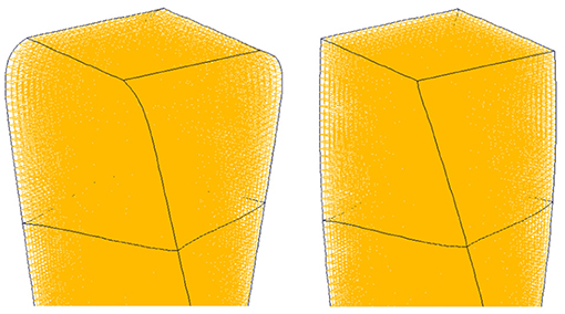
Figure A1. The end of a square beam deformed in torsion. The upper surface has been rotated 45° clockwise and the bottom surface 45° counter-clockwise. Version based on linear equations is shown on the left, and version based on non-linear equations is shown on the right.
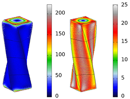
Figure A2. Shear stresses in a square beam with large torsionl deformations (the same 90° rotation as in Figure A1). Version based on linear equations is shown on the left, and version based on non-linear equations is shown on the right.
Deformations are best visualized when they are sizeable. The displacements involved in our calculations for the roughness exponent, on the other hand, are quite small. This is appropriate in a brittle fracture study, since the external displacements involved are usually small. Large deformations are more commonly associated with ductile materials. However, in order to illustrate a few cases of how stresses are altered as different modes of external loading are combined, we employ large displacements for visual effect. If we use Equations (15)–(20) for this purpose a “warping” effect is obtained when angular displacements become large. This is shown on the left in Figure A1, where the top and bottom surfaces have been rotated in opposite directions. Edges near the top and bottom are seen to turn inwards after a gradual swelling develops as the ends are approached. The reason why the effect is most marked near the ends is because it is here that rotational displacements are largest.
In contrast to this is the version shown on the right in Figure A1. Here, the axial contributions from the beams have been corrected to take into account the rotations about three axes. Components of shear and bending moment should also be adjusted in this way, leading to equations which involve a large number of terms. However, provided deformations are not too extreme, corrections applied to the axial terms are the most important. In Figure A1 the rotation of the top and bottom surfaces is 45 degrees, for a total rotation of 90 degrees between top and bottom. For such a large deformation the version on the right represents a dramatic improvement over the one on the left. The relevant modifications to Equations (15–17) are
for the X-component of force on node i,
for the Y-component, and
for the Z-component. Here
is the squared length of the discrete element between nodes i and j (disregarding curvature). Furthermore,
is the angular displacement of node i. As can be seen from Figure A1, the version on the right is clearly free of the warping seen in the version on the left.
The importance of taking into account local rotations for large deformations is made even more clear if we regard the stresses involved. In Figure A2 the shear stresses involved in the two cases are shown, and the color scales included with the beams illustrate the point. Evidently, when using linear equations, the stresses involved near the ends of the beam become quite extreme, almost 10 times higher than elsewhere in the beam. Away from the ends, however, the stresses are comparable, as can be seen from the color scales. In contrast, a uniform distribution of shear is obtained with Equations (1–3) in place of Equations (15–17).
The relevant equations are more complicated, and involve non-linear terms which necessitate an iterative adaption of conjugate gradients. In this approach the decreasing residuals of each successive solution are adopted as a starting point for a new tentative solution. Hence, at each stage in the breaking process a loop produces a sequence of tentative solutions. Within this loop, the number of iterations required for each successive solution decreases rapidly until the solution has converged. Although computational time increases significantly in comparison with the linear set of equations, it is still a only a matter of a minute or two to obtain stress distributions for relatively large structures. Such structures may be intact or at a pre-determined stage of breaking. However, for the purpose of studying the entire fracture process it is more practical to use linear equations in conjunction with small deformations.
We consider a beam in the form of a square prism, where all edges have been drawn black as an aid to emphasize body shape and displacements. External loads are imposed by rotating or translating the top and bottom surfaces of the body. The combination of bending and axial tension discussed in section 4 is illustrated in Figure A3 in the case of a beam with length 4L. Additional black lines in the figure delineate cubes with sides L = 25. On the left is a beam that is loaded in the vertical direction (stretched along the Z-axis), in the middle is the same beam in a bent configuration only (bending within the XZ-plane), and on the right the two loadings are combined. Stresses shown are axial stresses in discrete elements aligned along the vertical axis (the Z-axis). Referring to the color scale (the same scale relates to all three loadings) axial stresses of the tensile and bending cases are clearly seen to be additive, as expected from the superposition of forces in Equation (37).
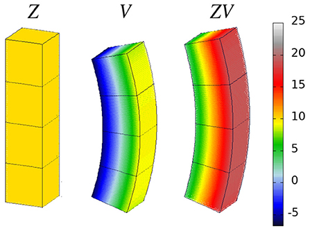
Figure A3. A square prism beam structure, sides L=25, and height H=101, loaded in tension (Z), pure bending (V), and the two combined (ZV).
In the figure, positive values are tensile while negative values are compressive. Average axial forces, obtained by summing from top to bottom along the middle of the vertical faces of the beam are included in Table A1. Here, ∑F090 and ∑F270 refer to the convex and concave sides of the beam, respectively, in Figure A3 The reason we consider average values of axial force is because we presently regard the 25 × 25 × 101 square prism as a model of a discrete element “beam.” In a fracture criterion we will not be interested in details pertaining to scales smaller than that of each element.
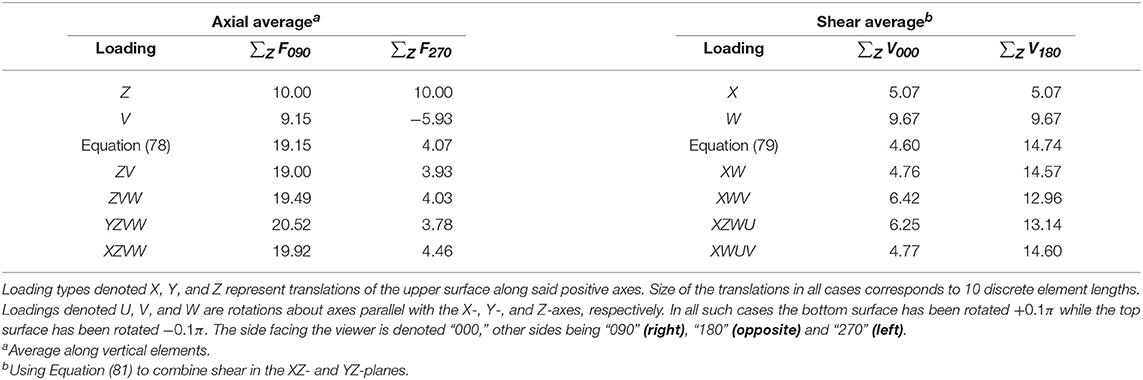
Table A1. Average forces summed from top to bottom along the middle of the vertical sides of a structure with square cross-section, sides L = 25 and height H = 101, with the structure having been subjected to different external loadings.
Table A1 shows that values obtained by adding “Z” and “V,” as dictated by Equation (78), agree well with the actual values obtained in the combined loading, denoted “ZV” in Figure A31. To what extent will additional loadings alter this picture? Instead of carrying out a systematic investigation involving many data points, a few extra loads added onto the “ZV” combinations have been included in the last three lines of Table A1. These are torsion, “ZVW,” as well as torsion and shear, “YZVW” and “XZVW.” In the latter cases the top surface has been translated along the positive Y- and X-axes, respectively. Although the displacements and rotations involving all the loadings are quite sizeable the average axial forces on the convex (∑F090) and concave (∑F270) sides do not change much, relatively speaking, as can be seen from the values in Table A1. Hence, the task of identifying the largest contribution from axial forces seems to be adequately taken care of by the first term, , in Equation (77). Had we considered the detailed distribution of forces rather than the averages, the highest axial force in the “YZVW” and “XZVW” cases would have been found to occur in discrete elements that are situated in the corners of the cross-section, near the top and bottom surfaces, on the concave side of the structure (see the color scale in Figure A4). Numerical values in these two cases are about 20% higher than the averages quoted in Table A1. Maximum axial stress in the “ZVW” case is only about 5% higher and occurs in a corner about three quarters of the way toward the top surface. In this context we also have to keep in mind that these values refer to cross-sections that are square rather than circular.
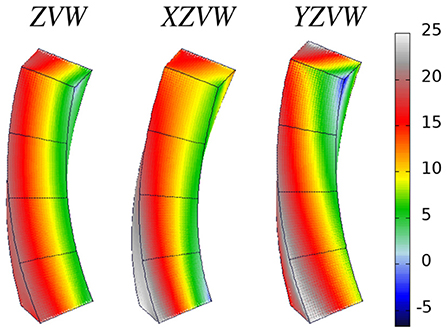
Figure A4. A square prism beam, with sides L=25, and height H=101, loaded in tension and bending (ZV), with added torsion (ZVW) and shear (XZVW and YZVW).
Table A1 also includes average shear forces calculated along the vertical faces of the square prism structure. Hence, the combination of shear and torsion, and to what extent this is affected by other loading modes, is investigated next. In Figure A5 is shown a beam under pure shear, pure torsion and the combination of these two loadings. The combined loading has been shown from three different angles, illustrating how shear on one side increases while that on the other side decreases, in accordance with the superposition of forces in Equation (79).
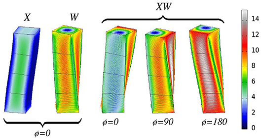
Figure A5. Beam of square cross-section, sides L = 25 and height H = 101, made up of discrete elements. The structure has been subjected to shear (X), torsion (W) and both these loadings combined (XW). Here, ϕ ≠ 0 is a counter-clockwise rotation of the structure. Hence ϕ = 90 has turned the side corresponding to toward the viewer.
On the extreme left is a beam where the top surface has been translated along the positive X-axis. The shear force is seen to be at its largest in the middle of the cross-section and decreases to zero at the edges. This is an example of Jourawski's formula, i.e.,
where
is the first, or static, moment of area about the axis of bending (the Y-axis in this case), Iy is the moment of inertia about the same axis, and L is the width of the cross-section. For a square cross-section the distribution of forces across the width is in the shape of a parabola. This is so because the external transverse force Vx produces a bending moment which varies along the length of the structure [98], i.e., the Z-axis in this case. The distribution of shear forces is shown in Figure A6 for a structure which has sides L = 25 and vertical length (or height) 8L. The external force Vx arises from a horizontal translation of the top surface a distance of 15 discrete elements. Numerical values are shown as solid squares and have been obtained along a line through the center of the cross-section, midway between the top and bottom surfaces. A parabola, shown in red, has been fit to these values. Apart from at the very edges, the numerical values are seen to conform very well to the shape predicted by Jourawski's formula. The discrepancy at the edges are finite-size effects, as can be seen by making finer the resolution of the discretization. Increasing proportionally the dimensions of the sample and the magnitude of the external deformation, the effect obtained is analogous to such a refinement of numerical resolution. One example of this is included in Figure A7, which shows the distribution of shear forces in a structure with sides L = 51 and height 8L. Here the external transverse displacement used corresponds to 30 discrete elements, and the discrepancy at the edges between the numerical values and the parabola is now seen to be much smaller.
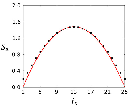
Figure A6. Shear force variation across the width of the mid-section of a 25 × 25 × 201 square beam, with parabola expression included for comparison shown in red.
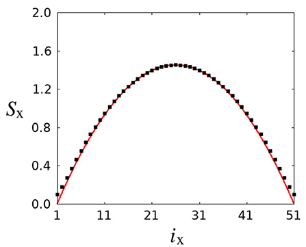
Figure A7. Shear force variation across the width of the mid-section of a 51 × 51 × 409 square beam, with parabola expression included for comparison shown in red.
The next beam in Figure A5, denoted “W,” is under pure torsion, and following this is the “XW” case where the two loadings “X” and “W” are combined. As expected, values in Table A1 obtained for the average forces on the sides where shear increases or decreases compare favorably with values expected from Equation (79), i.e., shear intensifies on one side and is alleviated on the other. The interesting question is to what extent other deformations influence this relationship. Adding a bending moment “V” or a biaxial bending moment “UV” changes the values somewhat (see Table A1, but not anywhere near what would be required to invalidate the relationship between “X” and “W” as incorporated into Equation (77) by the term . The distribution of forces involved when adding the biaxial moment “UV” are shown in Figure A8.
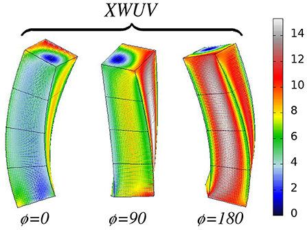
Figure A8. A square prism beam, with sides L = 25 and height H = 101, subject to shear (X), torsion (W) and biaxial bending (U and V).
The breaking thresholds for the two terms in Equation (77) have been set to the same value in Equation (80) since we wish to avoid making inferences about the detailed structure of each “beam.” If a “beam” is axially weak we also assume that it will be weak in shear, bending and torsion. We will not devise individual threshold distributions based on where “flaws” in a “beam” might be located. Otherwise one might, for instance, expect a “beam” with an edge crack to be unaffected in strength when bent such that the edge crack is compressed (closed) while weakened when it is bent the other way. Likewise, a “beam” with a central flaw might be expected to show structural resilience toward bending in either plane while being weakend in axial strength. We may still adjust the thresholds so that the “beam” is proportionally weaker in tension than in shear. This can be done, for instance, by multiplication with a constant factor. The main point is that all thresholds relevant to any given “beam” is chosen from a single value in the stochastic distribution.
Keywords: brittle fracture, stochastic media, discrete element model (DEM), fracture criteria, crack roughness
PACS numbers: 81.40.Np, 62.20.mt, 05.40.-a
Citation: Skjetne B and Hansen A (2019) Implications of Realistic Fracture Criteria on Crack Morphology. Front. Phys. 7:50. doi: 10.3389/fphy.2019.00050
Received: 14 November 2018; Accepted: 13 March 2019;
Published: 05 April 2019.
Edited by:
Daniel Bonamy, Commissariat à l'Energie Atomique et aux Energies Alternatives (CEA), FranceReviewed by:
Ferenc Kun, University of Debrecen, HungaryJonathan Bares, Université de Montpellier, France
Copyright © 2019 Skjetne and Hansen. This is an open-access article distributed under the terms of the Creative Commons Attribution License (CC BY). The use, distribution or reproduction in other forums is permitted, provided the original author(s) and the copyright owner(s) are credited and that the original publication in this journal is cited, in accordance with accepted academic practice. No use, distribution or reproduction is permitted which does not comply with these terms.
*Correspondence: Bjørn Skjetne, bjorn.skjetne@ntnu.no