 Vladimi L. Kulinskii
 Dmitry Yu Panchenko
94% of researchers rate our articles as excellent or good
Learn more about the work of our research integrity team to safeguard the quality of each article we publish.
Find out more
ORIGINAL RESEARCH article
Front. Phys., 02 April 2019
Sec. Statistical and Computational Physics
Volume 7 - 2019 | https://doi.org/10.3389/fphy.2019.00044
This article is part of the Research TopicContact Interactions in Quantum Mechanics: Theory, Mathematical Aspects and ApplicationsView all 16 articles
We consider singular self-adjoint extensions for the Schrödinger operator of spin-1/2 particle in one dimension. The corresponding boundary conditions at a singular point are obtained. There are boundary conditions with the spin-flip mechanism, i.e., for these point-like interactions the spin operator does not commute with the Hamiltonian. One of these extensions is the analog of zero-range δ-potential. The other one is the analog of so called δ(1)-interaction. We show that in physical terms such contact interactions can be identified as the point-like analogs of Rashba Hamiltonian (spin-momentum coupling) due to material heterogeneity of different types. The dependence of the transmission coefficient of some simple devices on the strength of the Rashba coupling parameter is discussed. Additionally, we show how these boundary conditions can be obtained from the Dirac Hamiltonian in the non-relativistic limit.
Point-like interactions can be described as the singular extensions of the Hamiltonian and are very useful quantum mechanical models because of their analytical tractability [1–5]. They are equivalent to some boundary conditions imposed on a wave function at the singular points and represent the limiting cases of field inhomogeneities. Therefore it is important to understand the relation between parameters of these BC and the specific physical characteristics of inhomogeneities. In modern nanoengineering the spin control is of great interest [6]. Besides the external magnetic field another interaction is the spin-momentum coupling which could be used for such a control [7, 8]. Thus the inclusion of magnetic field and other interactions which influence spin dynamics is a natural route for searching spin-dependent singular interactions. The interactions which influence spin polarization would give new examples of contact interactions with applications in condensed matter physics and QFT [9].
In non-relativistic limit spin s = 1/2 particle is described by the Pauli Hamiltonian [10]:
where σ represents the vector of Pauli matrices, is the external magnetic field and A, φ are vector and scalar potentials correspondingly. This Hamiltonian acts in space of 2-component wave functions:
Here ψ↑, ψ↓ are the wave functions of corresponding spin “up-” and “down-” states |↑〉, |↓〉. The probability current for Eq. (1) is as following:
where the last term describes the magnetization current (see e.g., [11]).
Bearing in mind the application to the 1-dimensional layered systems with spatial heterogeneity we use the conservation of current 3 to derive the boundary conditions (BCs) for the Hamiltonian 1 which model point-like interactions. We use the results of [12] where all possible self-adjoint BCs were related with the following Hamiltonian:
Here symbol Dx stands for the derivative in the sense of distributions on the space of functions continuous except at the point of singularity where they have bounded values along with their first derivatives [12, 13]:
The parameters Xi ∈ ℝ determine the values of the discontinuities of the wave function and its first derivative. The boundary conditions (b.c.) corresponding to each contribution in Eq. (4) can be represented in matrix form:
and conserve the current*
of the Hamiltonian
of a spinless particle. Physical classification of all these b.c. on the basis of gauge symmetry breaking was proposed in Kulinskii and Panchenko [14]. They can be divided into two subsets. The first one is formed by the matrices:
and can be associated with point-like interactions of electrostatic nature, e.g., standard zero-range potential is nothing but the limiting case of the potential field barrier. Another one is given by the BC matrices:
and represents the point-like interactions of the “magnetic” type. The parameters of 4 are related with the physical ones:
where is the mass-jump parameter and Φ is the magnetic flux (in units of Φ0 = 2πℏc/q). The magnetic nature of MX3 is obvious because of its interpretation as the localized magnetic flux. The last breaks the homogeneity of the phase of the wave function ψ. Also the scattering matrix of this b.c. has no time reversal symmetry [14].
The natural question arises as to the consideration of a particle with internal magnetic moment, e.g., a particle with spin s = 1/2. The very straightforward way for derivation of corresponding b.c. is the conservation of current Eq. (3). Therefore we introduce 4-vector (bispinor) of the boundary values at the singular point:
and boundary condition 4 × 4-matrix M:
Due to the structure of current Eq. (3) for the Hamiltonian 1 we have conservation of all its components:
Note that here we use expanded form of “curl” operator in Eq. (3) with explicit derivatives because we expect the discontinuity in their values. In fact, this the very form follows from the Dirac equation in non relativistic limit and the curl-operator appears after collecting the corresponding terms (see [10]). This point is important in view of X2-interaction which breaks the homogeneity of dilatation symmetry [15] because of the mass jump [14, 16]. In general Jy and Jz are different from zero even if we consider 1-dimensional case, e.g., layered system. The only demand consistent with the hermiticity of the Hamiltonian Eq. (1) is the conservation of current components Eq. (14). In terms of vector Φ the components of the probability current are as following:
where 4 × 4 matrices Σi are calculated by comparison of expressions Eqs. (14) and (15):
The conservation constraint of total current 15 gives the conditions for M-matrix:
Besides trivial solution for M-matrix consisting of two MX2, 3-blocks (no spin-flip), simple algebra gives the nontrivial 1-parametric solution of Eq. (18):
with
and b.c. of the form
This defines the spin-flip variant of X4-extension. E.g., corresponding scattering matrix for Mr is as following:
The scattering characteristics related to the scattering matrix Eq. (21) are in Figure 1.
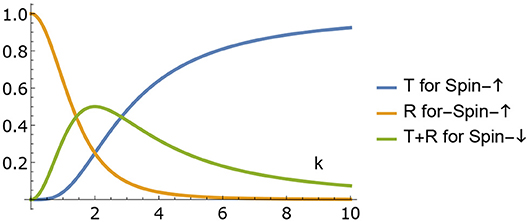
Figure 1. Scattering of |↑〉 - state on r−X4 defect.
Another solution of Eq. (18) is
with the b.c. of the form:
It can be considered as the δ-potential (X1-extension) augmented with the spin-flip mechanism. From the explicit form of the boundary conditions, e.g.,:
where MX2 is the block-diagonal matrix of X2-extensions. Thus the boundary condition for s = 1/2 particle with the spin-flip contact interaction can be written in general form:
Note that X3-extension can not be augmented with the spin-flip mechanism since it decouples from -couplings. In accordance with the spin-momentum nature of the r-couplings the physical reason of such factorization is that X3 contact interaction does not include spatial inhomogeneity in electric field potential φ. This is quite consistent with the difference between X2 and X3 from the point of view of breaking the gauge symmetry [14, 17].
Using the b.c. obtained above the standard test systems and their transport characteristics can be calculated straightforwardly in order to demonstrate spin-filtering properties. We give just two examples. First is the resonator (see Figure 2) for which the scattering amplitudes are in Figures 3, 4. Also we give the results of calculation of the resonant (quasilocalized) states (see Figure 5). Second is the filter (see Figure 6) with scattering characteristics are in Figure 7. The intensity of spin-flip process, generating the spin-↓ state from incident spin-↑ state is shown in Figure 3. These results demonstrate that spin-flip mechanism even at small values of r-coupling can reach high probabilities with increasing the energy of incident particle. Of course this directly follows from the boundary conditions (19) and (22) since the effects depend on both r and the momentum. Figure 4 represents the spin-flip effect for X1-resonator. Using such device it is possible to create the resonant (quasibound) states in the area between the wall and the defect (see Figure 5) for X4-filter. Comparison of and r−X4 cases shows that the last one is more effective as spin-flip mechanism.
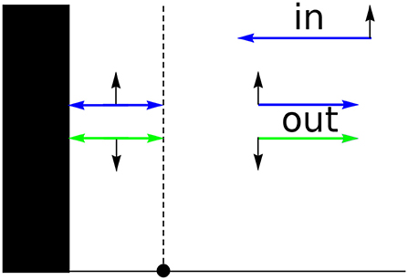
Figure 2. Resonator.
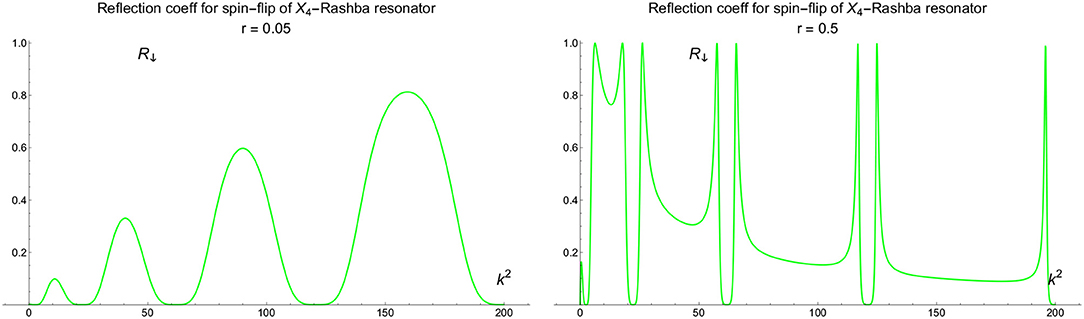
Figure 3. Intensity of reflected spin-↓ state for r−X4 resonator (see Figure 2) at different values of r.
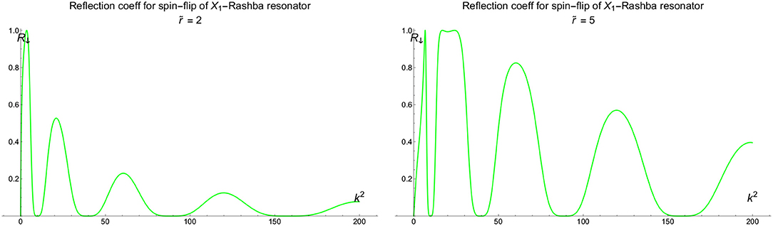
Figure 4. Intensity of reflected spin-↓ state for resonator (see Figure 2) at different values of .
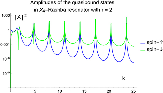
Figure 5. Amplitude of the wave function |↑〉, |↓〉-components in the resonant region.
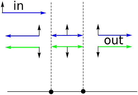
Figure 6. Filter.
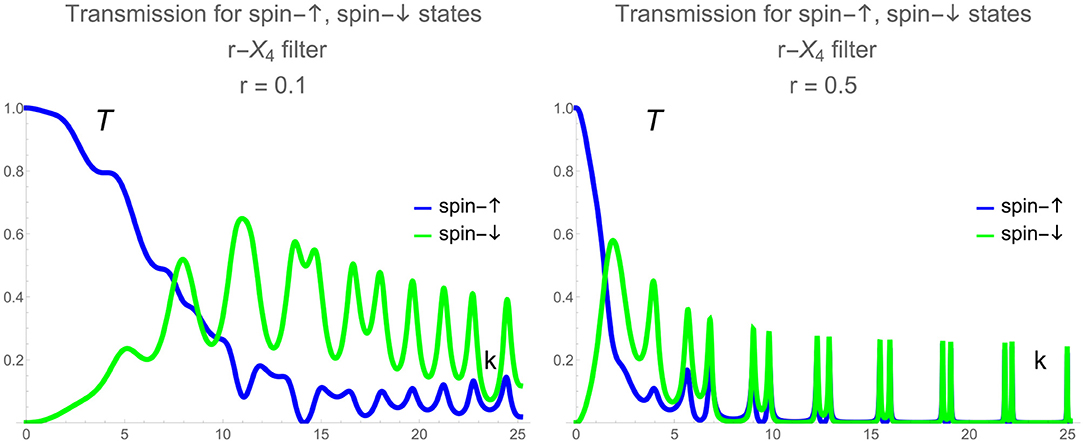
Figure 7. Transmission r−X4 filter intensity for different values of r.
The zone structure for periodic comb (see Figure 8) can be also calculated in standard way using Bloch representation of the wave function and imposing the corresponding b.c. In comparison with the spinless case considered in Albeverio et al. [3] here the spin degree of freedom doubles the number of zones (see Figures 9, 10). The corresponding dispersion laws are:
where q is the quasimomentum vector. Note that in case of X4-comb the lowest states belong to two parabolic zones with different effective masses at rX4 < 1:
At r = 1 one branch of excitations becomes massless:
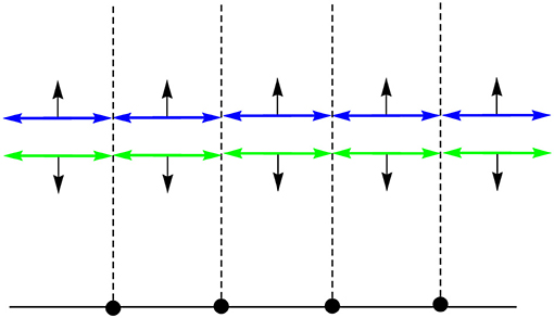
Figure 8. Comb structure.
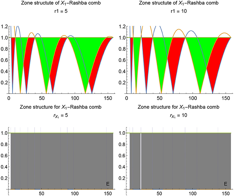
Figure 9. Zone structure of r−X1 - comb. Red and green are for “minus” and “plus” branches in Eq. (26) correspondingly.
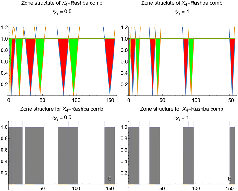
Figure 10. Zone structure of r−X4 - comb. Red and green are for “minus” and “plus” branches in Eq. (27) correspondingly.
Of course this is the remnant of what happens in standard X4-structure (see e.g., [3]). More intriguing problem here is the inclusion of the correlation effects due to spin statistics and investigation of phases with magnetic (dis)order in dependence on the intensity of point-like interactions. This way of research may be useful for modeling 1-dimensional magnetic systems [18].
As is known 3D case with the spherical symmetry can be effectively reduced to one dimensional problem on semi-axis r > 0 of the radial coordinate. Indeed let us define ϕ(r) = rψ(r) as the effective 1D wave function and consider natural definition domain of free Hamiltonian:
then the limiting value ϕ(0) as well as its derivative ϕ′(0) is defined since Eq. (30) is well defined on the corresponding Sobolev space which is dense in L2(ℝ+). The probability current is as following:
so the results for 1D case can be used. Introducing 2-spinor boundary-value vectors:
where
from Eq. (31) we get:
where W is the hermitean matrix. In standard decomposition on the Pauli matrices:
the scalar part (first term) corresponds to standard point-like potential b.c. [2, 19]:
and the states |↑〉, |↓〉 evolve independently. There is also spin-dependent repulsive/attractive version of 35:
which might be interpreted as the point-like potential with internal spin so that the sign of the potential depends on the spin-spin orientation of the particle and the center. The vector part (traceless second term) of Eq. (34) describes polarizational contact interactions with the spin-flip b.c.:
These b.c.'s in general describe how spin of an incident particle (e.g., an electron) interacts with the electrostatic potential localized at the singular point. In the absence of the external magnetic field the only mechanism for acting on spin in such situation is the relativistic spin-momentum coupling which we discuss in the following section.
The spin-flip point interactions introduced above make the spin operator no longer the integral of motion. There are two obvious physical origins for it (a) an external magnetic field with x, y-components and (b) spin-momentum coupling (Rashba coupling). The explicit k-dependence of the amplitudes of the spin-flip processes indicates that these interactions are due to spin-momentum coupling. Thus the physical interpretation of interactions represented by the b.c. matrices can be given in terms of the Rashba Hamiltonian [7, 8] (see also [20] and reference therein). Indeed, the Pauli Hamiltonian Eq. (1) as well as the current density Eq. (3) can be derived as the non relativistic limit for the Dirac Hamiltonian
where α = αi, i = 1, 2, 3 and β are the Dirac matrices
with I being 2 × 2 unit matrix. They act in the space of bispinors Ψ:
where spinors ξ and η represent particle and hole with respect to the Dirac vacuum states respectively [10]. The probability density is:
and in non relativistic limit transforms into
with
Here is the velocity operator. In the absence of external electromagnetic field this is equivalent to the following reduction of the bispinor in 1-dimensional case
so that the boundary element 4-vector 12 appears. Also we refer to the paper [21] where mass jump matching conditions were derived for the Dirac Hamiltonian in a graphen-like material where the velocity vF at the Fermi level serves as the speed of light.
The expansion of next order generates the spin dependent operator in the Hamiltonian:
It couples the spin with the momentum due to inhomogeneous background of the electric potential φ. In the limiting case of point-like interaction on the axis when ∇φ → 0 on both sides of the singular point this term drops out and should be interchanged with the boundary condition for the boundary vector 12 of the Pauli Hamiltonian 1. The conservation of the corresponding probability density current Eq. (3) provides self-adjointess of the boundary conditions for Eq. (1) in the presence of point-like singularity.
As a result, all extensions Xi, i = 1, 2, 4 which are singular limiting cases of the spatial distribution of the external electric field potential φ can be augmented with the spin-flip mechanism. Thus Eq. (25) defines the one-dimensional analog of the Hamiltonian with the point-like Rashba spin-momentum interaction [7].
The main result of the paper is that those extensions of the Schrödinger operator which are physically constructed on the basis of the inhomogeneous distribution of the electric field potential φ(x) can be augmented with the spin-flip mechanism. Note that in Eq. (24) both r-coupling and μ-parameter determine the spin-flip mechanism. This is in coherence with the results of Kulinskii and Panchenko [17] where X2 and X4 extensions were treated on the common basis of the spatial dependent effective mass. In its turn it is caused by the electrostatic field of the crystalline background. So it is not a surprise that these extensions can be combined through spin-momentum coupling in the Rashba Hamiltonian thus forming the “internal” magnetic field. In contrast to this pure “magnetic” X3-extension which is due to the external magnetic field does not couple with other Rashba point-like interactions.
Thus we can state that all point-like interactions δ, δ′-local and δ′-nonlocal (in terms of [22]) which are due to inhomogeneous electrostatic background can be augmented with the Rashba (spin-momentum) coupling. It is interesting to check this result independently using the Kurasov's distribution theory technique [12] and modified correspondingly for spin 1/2 case. Also we expect that such b.c.'s can be related to the zero-range potential models with the internal structure of the singular point studied in Pavlov [23]. This will be the subject of future work.
VK and DP conceived of the presented idea. VK proposed physical interpretation for the spin-flip matching conditions. VK encouraged DP to investigate the possibility to derive them based on the Dirac Hamiltonian and supervised the findings of this work. All authors discussed the results and contributed to the final manuscript.
This work was completed due to MES Ukraine grants 0115U003208, 018U000202 and the individual (VK) Fulbright Research Grant (IIE ID: PS00245791). VK is also grateful to Mr. Konstantin Yun for financial support of the research.
The authors declare that the research was conducted in the absence of any commercial or financial relationships that could be construed as a potential conflict of interest.
The authors thank Prof. Vadim Adamyan for clarifying comments and discussions.
*. ^here we put ℏ = 1, c = 1 and m = 1/2.
1. Demkov YN, Ostrovsky V. Zero-Range Potentials and Their Applications in Atomic Physics. New York, NY: Plenum (1988).
2. Baz' AI, Zeldovich YB, Perelomov AM. Scattering Reactions and Decays in Non-Relativistic Quantum Mechanics, 1st ed. Jerusalem: Israel Programm for Scientific Transaction (1969).
3. Albeverio S, Gesztesy F, Høegh-Krohn R, Holden H. Solvable Models in Quantum Mechanics. New York, NY: Springer-Verlag (1988).
4. Adamyan VM, Pavlov BS. Null-range potentials and M. G. Krein's formula for generalized resolvents. J Math Sci. (1988) 42:1537–50. doi: 10.1007/BF01665040
5. Albeverio S, Kurasov P. Singular Perturbations of Differential Operators. Solvable Schrodinger Type Operators, London Mathematical Society Lecture Note Series, Vol. 221. Cambridge: Cambridge University Press (2000).
6. Datta S, Das B. Electronic analog of the electro-optic modulator. Appl Phys Lett. (1990) 56:665–67. doi: 10.1063/1.102730
7. Rashba E. Properties of semiconductors with an extremum loop. 1. cyclotron and combinational resonance in a magnetic field perpendicular to the plane of the loop. Sov Phys Solid State. (1960) 2:1109–22.
8. Bychkov YA, Rasbha EI. Properties of a 2d electron gas with lifted spectral degeneracy. P Zh Eksp Teor Fiz. (1984) 39:66.
9. Nieto L, Gadella JM, Mateos Guilarte M, Munoz-Castaneda JM, Romaniega C. Towards modelling QFT in real metamaterials: singular potentials and self-adjoint extensions. J Phys. (2017) 839:012007. doi: 10.1088/1742-6596/839/1/012007
10. Berestetskii V, Lifshitz E, Pitaevskii L. Course of Theoretical Physics, Volume IV: Quantum Electrodynamics. Oxford: Butterworth-Heinemann (1981).
11. Landau LD, Lifshitz LM. Course of Theoretical Physics, Volume III: Quantum Mechanics (Non-Relativistic Theory). Oxford: Butterworth-Heinemann (1981).
12. Kurasov P. Distribution theory for discontinuous test functions and differential operators with generalized coefficients. J Math Anal Appl. (1996) 201:297–323. doi: 10.1006/jmaa.1996.0256
13. Kurasov P, Boman J. Finite rank singular perturbations and distributions with discontinuous test functions. Proc Am Math Soc. (1998) 126:1673–83. doi: 10.1090/S0002-9939-98-04291-9
14. Kulinskii V, Panchenko D. Physical structure of point-like interactions for one-dimensional Schrödinger and the gauge symmetry. Physica B. (2015) 472:78–83. doi: 10.1016/j.physb.2015.05.011
15. Albeverio S, Dabrowski L, Kurasov P. Symmetries of Schrödinger operators with point interactions. Lett Math Phys. (1998) 45:33–47. doi: 10.1023/A:1007493325970
16. Gadella M, Kuru S, Negro J. Self-adjoint hamiltonians with a mass jump: general matching conditions. Phys Lett A. (2007) 362:265–8. doi: 10.1016/j.physleta.2006.10.029
17. Kulinskii V, Panchenko D. Mass-jump and mass-bump boundary conditions for singular self-adjoint extensions of the Schrödinger operator in on dimension. ArXiv e-prints. (2018).
18. Mikeska HJ, Kolezhuk AK. One-Dimensional Magnetism. Berlin, Heidelberg: Springer Berlin Heidelberg (2004).
19. Berezin FA, Faddeev LD. A remark on Schrödinger's equation with a singular potential. Sov Math Dokl. (1961) 2:372–5.
20. Manchon A, Koo H, Nitta J, Frolov S, Duine R. New perspectives for rashba spinorbit coupling. Nat Mater. (2015) 14:871–82. doi: 10.1038/nmat4360
21. González-Diaz L, Diaz AA, Diaz-Solózano S, Darias JR. Self-adjoint dirac type hamiltonians in one space dimension with a mass jump. J Phys A Math Theor. (2015) 48:045207. doi: 10.1088/1751-8113/48/4/045207
22. Fassari S, Gadella M, Glasser M, Nieto L. Spectroscopy of a one-dimensional v-shaped quantum well with a point impurity. Ann Phys. (2018) 389:48–62. doi: 10.1016/j.aop.2017.12.006
Keywords: Schrödinger operator, self-adjoint extension, Rashba interaction, spin-flip, Pauli Hamiltonian, Dirac Hamiltonian
Citation: Kulinskii VL and Panchenko DY (2019) Point-Like Rashba Interactions as Singular Self-Adjoint Extensions of the Schrödinger Operator in One Dimension. Front. Phys. 7:44. doi: 10.3389/fphy.2019.00044
Received: 16 December 2018; Accepted: 08 March 2019;
Published: 02 April 2019.
Edited by:
Manuel Gadella, University of Valladolid, SpainReviewed by:
Silvestro Fassari, Universitá degli Studi Guglielmo Marconi, ItalyCopyright © 2019 Kulinskii and Panchenko. This is an open-access article distributed under the terms of the Creative Commons Attribution License (CC BY). The use, distribution or reproduction in other forums is permitted, provided the original author(s) and the copyright owner(s) are credited and that the original publication in this journal is cited, in accordance with accepted academic practice. No use, distribution or reproduction is permitted which does not comply with these terms.
*Correspondence: Vladimi L. Kulinskii, a3VsaW5za2lqQG9udS5lZHUudWE=
Disclaimer: All claims expressed in this article are solely those of the authors and do not necessarily represent those of their affiliated organizations, or those of the publisher, the editors and the reviewers. Any product that may be evaluated in this article or claim that may be made by its manufacturer is not guaranteed or endorsed by the publisher.
Research integrity at Frontiers
Learn more about the work of our research integrity team to safeguard the quality of each article we publish.