 Thomas Curtright1,2*
- 1Physics Department, University of Florida, Gainesville, FL, United States
- 2Department of Physics, University of Miami, Coral Gables, FL, United States
We discuss a set of local fields which provide the on-shell massless states expected for the fundamental linear representation of supersymmetry in twelve dimensions. We recover the states of the anticipated N = 16, S = 4, massless supermultiplet upon reduction to four dimensions. Using algebraic methods, we also construct ghost arrays which permit the covariant quantization of each of the gauge fields in the set.
Introduction
Using group theoretic methods, Nahm [1] has established that all linear representations of supersymmetry in D > 11 dimensions will give rise to fields with spins greater than two when reduced to four dimensions. That is, simple supergravity cannot exist if D is greater than eleven. A set of local fields which realize supergravity when D = 11 is now well-known from the seminal work of Cremmer et al. [2].
Perhaps it is still not always appreciated, however, just how truly economical D = 11 supergravity is. Consider the following properties of the “fundamental” massless supermultiplet [1]. Increasing the dimension raises the number of physical degrees of freedom from 256, for D = 11, to 65536, for D = 12, and raises the maximum “helicity” content from S = 2, for D = 11, to S = 4, for D = 12. This considerable enlargement of the fundamental supermultiplet for D = 12 can be understood by noting that the smallest (Majorana or Weyl) spinor field in twelve dimensions carries 32 massless degrees of freedom on-shell. Ultimately, this results in N = 16 separate supersymmetries upon reduction to four dimensions, with a corresponding manifest 0(16) global invariance.
The major increase in the size of the smallest supermultiplet, in going from D = 11 to D = 12, might not be so undesirable, except that there is no known way to construct a completely consistent, locally interacting theory involving fields with S > 2. In fact, there are a number of “no-go” theorems which, taken at face value, indicate that higher spin local field theories are incurably sick. (For an example of such a theorem, see Weinberg and Witten [3]. For a review of higher spin problems around that same time, see Curtright [4].)
Nonetheless, in this paper we shall adopt a constructive point of view based on the following remarks. Although the fundamental D = 12 supermultiplet is large, it is expected to exist as a well-defined free field theory with interesting kinematical structure, and it deserves to be explicitly discussed in the literature, at the very least for purposes of comparison with D = 11 supergravity. In addition, if higher spin local fields have any natural setting, surely it is within the context of N > 8 extended supersymmetric models where the symmetry alone requires at least one spin as high as S = N/4 for the fundamental linear supermultiplet. Drawing a lesson from N = 8 supergravity, the most elegant and natural formulation of such models is probably in higher dimensions. Finally, it is possible that the local fields appearing in massless D = 12 supermultiplets may play a role as auxiliaries in lower dimensional theories. Thus, we shall exhibit here an elementary local field candidate for the fundamental D = 12 supermultiplet.
First, we give a set of local fields which have the correct on-shell states appropriate for the massless D = 12 fundamental supermultiplet. All but two of the members of this set are “maximal” gauge fields, with rather exotic local symmetries. Next, we discuss reduction of the multiplet from D = 12 to D = 11 and lower dimensions, and explain how the N = 16, S = 4 multiplet arises upon going to D = 4. Then, using algebraic methods, we initiate the covariant quantization of the gauge fields contained in the proposed supermultiplet by constructing an acceptable ghost array for each field. Finally, we conclude with some conjectures concerning the uses of such a high spin supermultiplet. In particular, it could also be interpreted as a massive bound-state multiplet for D = 11 supergravity.
Candidate Local Fields
Massless fields in Twelve dimensions describe on-shell states which are representations of the transverse orthogonal group 0(10). We shall decompose these on-shell representations into irreducible ones (“irreps”), and label the latter by their highest weights [standard group theoretic notation [5]]. Since 0(10) has rank five, these weights are vectors in a five-dimensional Euclidean space: (w1, w2, w3, w4, w5). In addition, we shall sometimes use subscripts and superscripts, respectively, to denote the dimensions and second indices (divided by 5) of the 0(10) irreps:
Note that the two irreps related by interchange of their spinor labels, i.e., (wl,w2,w3,w4,w5) and (wl,w2,w3,w5,w4), have equal dimensions and indices of all orders.
We shall label the fields carrying these 0(10) representations by a Young pattern of 0(11, 1) Lorentz indices (a, b, c, …), using “R” for the real tensors, “C” for the complex tensors, and “ψ” for the (Majorana or Weyl) spinor-tensors. By convention, any rows of Lorentz indices are first totally symmetrized, and then any columns of indices are totally antisymmetrized. Dirac indices on the spinor fields will always be suppressed. When we list a real representation for a complex field, both real and imaginary parts of the field are understood to carry such a real representation independently. With these conventions, the local fields we propose to describe the fundamental D = 12 supermultiplet are listed in Table 1. Only two of these fields are obvious, (40000) and (30001) + (30010), since we expect one S = 4 and 16 S = 7/2 states upon reduction to D = 4. The other entries in Table 1 were determined essentially by trial and error.
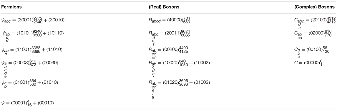
Table 1. D = 12 Local fields and their massless 0(10) on-shell states.
Note that in Table 1, all the spinor-tensor fields, and two of the real tensor fields, reduce on-shell to a pair of 0(10) irreps. It is also remarkable, but certainly not surprising, that essentially all entries in Table 1 are generalized gauge fields [6, 7]. Only two fields, ψ and C, lack local gauge transformations. Some of the local gauge transformations for the other fields in the Table are rather exotic. We will say more about this later when we discuss covariant quantization and ghosts.
As a preliminary check that these fields form the alledged D = 12 supermultiplet, we observe that the sums of dimensions, and second indices, over all the bosons are precisely equal (= 32768) to the same sums over the fermions. These are examples of “spin-moment” sum rules for supermultiplets [8], generalized to higher dimensions [9]. For the present case, supersymmetry requires agreement between index sums over bosons and index sums over fermions up to but excluding the sixteenth order1. Note that it is not difficult just to match dimensions for the boson and fermion representations by using a smaller set of fields [6, 10]. This trivial match, however, is grossly insufficient to guarantee supersymmetry.
Dimensional Reduction
Another check on the supersymmetry of the field multiplet is obtained by reducing from D = 12 to D = 11. The physical 0(10) states then branch into 0(9) representations as shown in Table 2. Since 0(9) has rank 4, the 0(9) irreps are characterized by four-dimensional weight vectors as shown. The 0(9) states listed in Table 2 may be grouped into simple D = 11 supermultiplets. In fact, one readily identifies the 0(9) states in Table 2 as just those obtained by “squaring” the physical state representations of the fundamental D = 11 supermultiplet: { (2000), (0010), (1001) }.
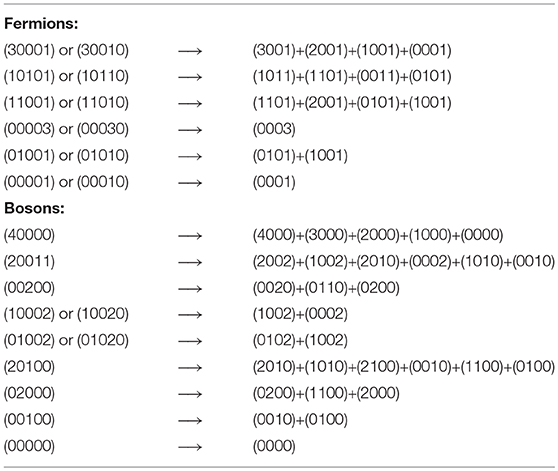
Table 2. 0(10) → 0(9) Branching of massless on-shell states upon reducing D = 12 → D = 11.
The D = 12 → D = 11 reduction and 0(10) → 0(9) branching procedure can also be turned around as follows. First, square the physical 0(9) states for the fundamental D = 11 supermultiplet. Then, embed the resulting representations in 0(10) irreps. Finally, identify those 0(11, 1) fields which yield these 0(10) irreps on-shell. (In practice, the second and third steps may require a bit of educated guess-work.) This inverted procedure can usually be successfully employed to raise D, but note that it may sometimes fail. For example, suppose one trys to raise D = 10 to D = 11, starting with the fundamental D = 10 supermultiplet whose physical on-shell states are the 0(8) irreps { (1000), (0001) }. Simply squaring these states does not give a set of representations which can be expressed as an eleven dimensional theory. Rather, one obtains the states of a type-II, D = 10 superstring [11]: { (2000), 2(0000), 2(0100), (0002), 2(0010), 2(1001) }. To obtain the states corresponding to D = 11 supergravity, one must multiply { (1000), (0001) } by { (0000), (0010) } where (0001) has been replaced by the inequivalent spinor (0010).
Having shown how the D = 12 fields reduce to give D = 11 states appropriate for supermultiplets, it follows that further dimensional reduction, say to D = 4, must also give the correct states for supermultiplets. Nevertheless, there are some slight subtleties encountered if one simply takes the D = 12 fields in Table 1 and reduces. The S = 4 singlet, S = 7/2 16-plet, and S = 3 120-plet are all easily found among the D = 12 → D = 4 fields. Lower spins may appear to be too plentiful, however. To correctly count lower spins, one should consider the free field action. As a simple illustration, reduce a maximally gauge invariant Dirac spinor-tensor, , from D = 5 to D = 4. Altogether, there must be zero physical (propagating) states both before and after the reduction, but naively, there appear to be D = 4 propagating modes corresponding to a spin 3/2 field, (a = 1, 2, 3, 4). Those spurious states are immediately dismissed by inspection of the appropriate D = 5 Lagrangian, which in this case is . Similarly, when carefully done, complete reduction fields in Table 1 from D = 12 to D = 4 gives the correct set of physical N = 16, S = 4 supermultiplet.
Ghost Arrays and Maximal Gauge Invariance
Next, let us consider some aspects of the covariant quantization of the gauge fields in Table 1. We exhibit in Table 3 arrays of ghost fields which are needed to carry out such a quantization. In the first column of Table 3 we again list the physical on-shell 0(10) irreps carried by the D = 12 local fields of Table 1. In the second column, we list the 0(12) irreps which describe the gauge fields, and their ghost fields, off-shell. (It is unnecessary here to distinguish 0(12) and 0(11, 1).) For each entry in column 1 of Table 3, the initial row of the corresponding entry in column 2 consists of the off-shell 0(12) irreps carried by the primary gauge field itself (whose Young pattern appears in Table 1). For example, Rabcd is reducible and carries the irreps (400000) + (200000). The second irrep is simply the trace, Rabcc (Note that this field has no double trace, Raacc = 0.)
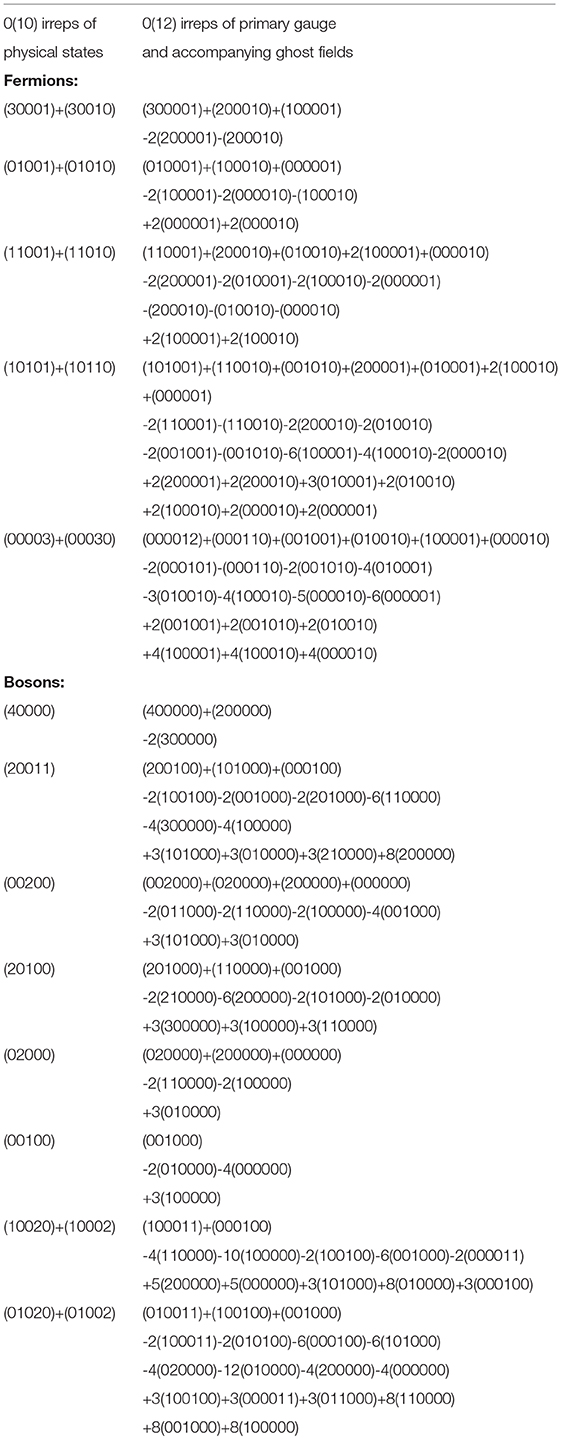
Table 3. Gauge field and ghost arrays.
The other rows in column 2 describe the ghosts. Those with minus signs have “wrong” statistics. Again considering Rabcd as an example, “−2(300000)” signifies two anticommuting, real, traceless, symmetric rank 3 tensor ghost fields. On the other hand, ghosts with plus signs have “right” statistics. These “+” ghosts (and some of the “−” ghosts as well) are actually “ghosts for ghosts” required by the subsidiary local gauge invariances of other ghosts [12–15]. This last statement may be somewhat confusing, so let us indicate how the ghosts may be obtained very quickly using algebraic methods.
No matter how elaborate, all ghost arrays can be constructed by simple numerical methods involving elements in a representation ring. One begins with the familiar structure for a vector field. For D = 12, this may be written as
That is, the physical 0(10) states may be viewed as a difference (hence representation ring) of 0(12) vector and scalar irreps, the latter being the usual Faddeev-Popov ghosts. To obtain the ghost structures for other, higher rank gauge fields, one must define appropriately symmetrized products of both sides of Equation (1). For example,
The LHS of this equation is obviously
The RHS of Equation (2) is not so obvious, however. Anticommutativity of the local ghost fields must be correctly incorporated into the definition of symmetrized products of the ghost 0(12) irreps. Here, it suffices to give an operational definition of arbitrarily symmetrized products of the full RHS of Equation (1), in terms of an algorithm.
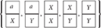
The algorithm goes as follows. First, construct Young patterns of Lorentz indices corresponding to appropriately symmetrized products of the (100000)'s which come from the RHS of Equation (1). Then, remove Lorentz indices from these patterns in all possible ways by substituting for individual Lorentz indices, a, b, c, …, either an “X” or a “Y”, corresponding to the two ghosts in Equation (1). Incorporate the anticommutativity of those ghosts using the rule that neither two X's nor two Y's can be used to remove a symmetric pair of Lorentz indices. Next, identify the 0(12) irreps corresponding to the various Young patterns which arose from removing Lorentz indices by these “ghost insertions”. Finally, a resulting 0(12) irrep has right/wrong statistics if an even/odd number of Lorentz indices were removed to obtain that irrep.
For the example in Equation (2), ((100000)⊗(100000))symmetric = (200000) + (000000). The application of the algorithm to (200000) gives: (200000) →  →
→  → {−(100000), −(100000), +(000000)}. Thus, using the algorithm, the RHS of Equation (2) is
Upon canceling a common, commuting singlet field from both sides of Equation (2), (00000) = (000000), we obtain
One immediately recognizes the well-known pair of vector ghosts employed in the covariant quantization of a symmetric rank 2 tensor field (gravity). The first two terms on the RHS of Equation (3) are just the 0(12) irreps into which the reducible metric tensor decomposes (i.e. (000000) is the off-shell trace of the graviton field).
As another example, we take the antisymmetric square of Equation (1).
Applying the algorithm to the RHS of this equation gives: (010000) →  →
→  → {−2(100000), +3(000000)}. Thus, we obtain
An antisymmetric rank 2 tensor requires two vector ghosts which in turn require three scalar ghost-ghosts [12]. The latter are commuting fields.
At this point, further generalizations should be obvious. In particular, all the entries in Table 3 follow from these simple algebraic considerations2. Spinor-tensors are treated by multiplying both sides of tensor equations (such as Equation (1)) by the elementary spinor result: (00001) + (00010) = (000001) or (000010). Note that this always yields 0(10) spinor irreps in pairs of the form (wl, w2, w3, w4, w5) + (wl, w2, w3, w5, w4). Fortunately, all the physical 0(10) states occurring in Tables 1, 3 are so paired, including multi-spinor irreps such as (10020) + (10002) (i.e., this 0(10) irrep of physical states is not (anti)self-dual). In fact, it has been argued that such (multi-)spinor pairing is necessary in order to have a covariant formulation for a gauge field [18]. From a group-algebraic point of view, this is a direct consequence of embedding O(D−2) into O(D).
There is an extra interesting feature about the ghosts for each of the spinor-tensors in Table 3. For example, consider ψabc. Naively, it appears in Table 3 that the representation (200010) is simply canceled by −(200010) occurring in the adjacent line. One can in effect cancel out these fields, and subsequently ignore them, if a certain type of gauge is selected, but in a general gauge one cannot. This additional ghost was first discussed by Nielsen in the context of spin 3/2 fields in four dimensions [19]. At issue is simply the reducibility, in a general gauge, of the spinor-tensor ψabc when considered as an 0(12) representation. In general, the field has a Dirac trace, γaψabc (but note that, as defined in Table 3, ψabc is always without a triple Dirac trace, γaγbγcψabc = 0)3. Similar remarks obviously hold for the other spinor-tensors in Table 34.
There are some simple numerical checks that one can perform for the ghost arrays in Table 3 which are similar to checking supersymmetry by matching fermion and boson representation index sums. First, the net dimension of the 0(10) irreps in column l of Table 3 must agree with the net dimension of the 0(12) irreps in column 2 (subtract dimensions of the “–” ghosts, add all other dimensions). Secondly, the net second index of the 0(10) irreps, divided by the rank of 0(10) (= 5), must equal the net second index of the 0(12) irreps, divided by the rank of 0(12) (= 6). One easily verifies these checks on Table 3 using the numerical results in McKay and Patera [5].
The above change of scale (i.e., group rank) in comparing second indices is physically significant for computing quantum corrections. Unitarity requires that covariant evaluations of closed loops using the 0(12) gauge field and ghost irreps give the same results as dispersive evaluations of closed loops using the physical 0(10) irreps as on-shell intermediate states. This unitarity constraint can be satisfied if such loop evaluations depend on the ratio “second index/rank”, as is the case in a simple example [9].
To end this discussion of Table 3, we explain the character of the local gauge transformations for the primary gauge fields. These gauge fields are all “maximal” in the following sense. The local variation of any such (spinor-)tensor field of rank “r”' is just a gradient of a general local gauge parameter (spinor-)tensor of rank “r−1”, with all Lorentz indices appropriately symmetrized after the gradient is taken, to conform to the original symmetry pattern of the primary gauge field. The only constraints possibly to be imposed on the local gauge parameters are simple “zero trace” conditions (cf. [4] for a guide to the earlier literature on this subject). For example, for the primary gauge field Rabcd, the rank 3 local gauge parameter, rabc, has no trace, raac = 0.
This trace condition, and any others, actually follows from Table 3, if the local gauge transformations are written in BRST form. In that form, a local gauge parameter is expressed as a local ghost field multiplying a global scalar parameter. Any trace constraints are then carried by the ghost 0(12) representation. For the Rabcd example, (300000) denotes a traceless, symmetric, rank 3 ghost. Hence the corresponding local gauge parameter is traceless. Similarly, it follows that trace conditions on local gauge parameters for other high rank (spinor-)tensor fields can be deduced rather easily as a by-product of the simple numerical analysis used to construct their ghost arrays, starting from Equation (1). By postulating maximal gauge invariance, the free field Lagrangians may be uniquely determined (up to trivial field redefinitions) for all the gauge fields in Table 3. This remark summarizes a straightforward, but tedious exercise which will not be given in detail here, to avoid unnecessarily straying from our group-algebraic line of development.
Possible Applications and Open Questions
In conclusion, we briefly consider possible applications of the local fields given in the Tables. Obviously, consistent interactions are required before these fields can be used to describe physical states in a model. Consistent local interactions among all these fields are not known, and for reasons reviewed in Curtright [4], probably do not exist for most of the fields when they are massless. Still, this leaves open two logical possibilities: nonlocal interactions, or massive fields. Conceivably, both of these options may need to be used simultaneously. (Recall dual resonance models as high spin theories [20, 21].)
Let us consider some consequences of allowing the local fields to be massive. Viewed as on-shell states for massive D = lZ fields, the individual 0(10) representations in the Tables are incomplete: longitudinal modes are missing. One could remedy this by simply adding the missing states necessary to form complete 0(11) irreps. However, a more interesting possibility is simply to keep the original 0(10) irreps in Table 1 and interpret them as on-shell states for massive D = 11 fields. Such a massive multiplet of D = 11 fields is of interest in D = 11 supergravity. (The multiplet in Table 1 is not the supercurrent multiplet, but it can be used to directly obtain that multiplet through successive multiplications by two 0(10) vector irreps, (10000).) It is unknown whether or not such a massive multiplet could be dynamically realized as bound states for D = 11 supergravity. (Perhaps related to this, such a multiplet might provide some of the auxilliary fields for the D = 11 theory.) One way to study this possibility would be to generalize to higher dimensions previous work on the Reggeization of N = 8 supergravity [22]. Note that in general, the logical extension of Regge theory to higher dimensions would require “highest-weight-vector” trajectories, if on-shell states are to be unambiguously specified along the trajectories.
Finally, regarding local interactions, it is an open question whether or not massive higher rank D = 11 fields (such as those obtained by re-interpreting Table 1) can consistently and locally couple to D = 11 supergravity. To completely answer this question, one would have to examine all possible local nonmininal gravitational couplings for those fields. Local nonminimal couplings are indeed suggested by the local conformal energy-momentum tensor improvements known to exist for massive tensor fields which are not totally symmetric in their Lorentz indices [7]. By way of contrast, such conformal improvements cannot be locally constructed in a gauge invariant way [23] for massless, generalized gauge fields5.
Added Comments
The above was written some 36 years ago, and preprinted but unpublished in a journal at that time. It is offered here to make the historical record more accessible.
I have modified the preceding text only in the final section to include citations of two papers written subsequently, namely, Curtright and Thorn [20] and Curtright [21]. One of the reviewers for this journal suggested that a connection may exist between this work and F-Theory[24–26]. I believe that such a connection, if it exists, is outside the scope of this paper. In fairness to other, more recent work, I should also mention here efforts to develop supergravity models in twelve dimensions involving two times [27]. While such models fall outside Nahm's classification, nevertheless I am led to suspect there might be a link to the discussion above.
In addition, there has been recent progress on constructing interacting theories involving higher spins, and this work is continuing [28]. Finally, as evident from the other contributions to this issue of Frontiers, work also continues on generalized gauge fields, especially in the context of dual gravity.
Author Contributions
The author confirms being the sole contributor of this work and has approved it for publication.
Conflict of Interest Statement
The author declares that the research was conducted in the absence of any commercial or financial relationships that could be construed as a potential conflict of interest.
Acknowledgments
I thank Professor P. Ramond for several discussions about higher dimensional supermultiplets. This work was supported in part by the Department of Energy, under contract number DSR80136je7.
Footnotes
1. ^For the fields in Table 1, we have only checked the matching of fermion and boson index sums up to sixth order.
2. ^It facilitates the determination of ghosts for other examples to use Schur-function division. One divides the S-functions corresponding to physical state irreps by the S-functions generated by the formal series . Not surprisingly, this is the formal inverse of the operation which reduces O(D) to O(D − 2) [see King [16]]. Division of S-functions is explained and many specific examples are given in Wybourne [17]. I am indebted to Professor Wybourne for discussions about S-functions, especially for suggesting that S-function division might be useful for this problem, and for bringing this literature to my attention.
3. ^Note, if a gauge like γaψabc = 0 is chosen, one must re-introduce as an independent field the irrep (100001) that appears in Table 3.
4. ^Note that right statistics, even-order insertions of the fundamental Faddeev-Popov ghosts, “X” and “Y”, may be directly carried by higher rank primary gauge fields in the form of even-order Dirac, or metric traces. Nielsen ghosts are wrong statistics, odd-order insertions of the fundamental Faddeev-Popov ghosts, and are used to cancel odd-order Dirac traces of primary spinor gauge fields. Note that there are also examples of Nielsen ghosts for ghosts in Table 3.
5. ^Local on-shell improvements do exist in certain gauges. Thus, arbitrary gauges require nonlocal modifications for the conformal improvement of the classical energy-momentum tensor. This would seem to be compatible with a conjecture that massless generalized gauge fields can couple consistently (e.g., gauge invariantly) to gravity if nonlocal effects are incorporated.
References
1. Nahm W. Supersymmetries and their representations. Nucl Phys. (1978) B135:149–66. doi: 10.1016/0550-3213(78)90218-3
2. Cremmer E, Julia B, Scherk J. Supergravity in theory in 11 dimensions. Phys Lett. (1978) 76B:409–12. doi: 10.1016/0370-2693(78)90894-8
3. Weinberg S, Witten E. Limits on massless particles. Phys Lett. (1980) 96B:59–62. doi: 10.1016/0370-2693(80)90212-9
4. Curtright TL. High spin fields. In: Durand L, Pondrom LG. editor. Proceedings, XXth International Conference on High Energy Physics. Madison, WI: AIP (1980). pp. 985–8. Available online at: https://www.amazon.com/High-Energy-Physics-1980-International-Conference/dp/B000OV7B7U/ref=sr_1_1?s=books&ie=UTF8&qid=1530920078&sr=1-1&keywords=Durand+and+Pondrom
5. McKay W, Patera J. Tables of Dimensions, Indices and Branching Rules for Representations of Simple Lie Algebras, New York, NY: Dekker (1981). Available online at: http://www.worldcat.org/title/tables-of-dimensions-indices-and-branching-rules-for-representations-of-simple-lie-algebras/oclc/7168656
6. Curtright TL. Generalized gauge fields. Phys Lett. (1985) 165B:304–8. doi: 10.1016/0370-2693(85)91235-3
7. Curtright TL, Freund PGO. Massive dual fields. Nucl Phys. (1980) B172:413–24. doi: 10.1016/0550-3213(80)90174-1
8. Curtright TL Charge renormalization and high spin fields. Phys Lett. (1981) 102B:17–21. doi: 10.1016/0370-2693(81)90203-3
9. Curtright TL. Indices, triality, and ultraviolet divergences for supersymmetric theories. Phys Rev Lett. (1982) 48:1704–8. doi: 10.1103/PhysRevLett.48.1704
10. Castellani L, Fre P, Giani F, Pilch K, van Nieuwenhuizen P, Beyond d=11 supergravity and cartan integrable systems. Phys Rev. (1982) D26:1481. doi: 10.1103/PhysRevD.26.1481
11. Green MB, Schwarz JH, Supersymmetrical string theories. Phys Lett. (1982) 109B:444–8. doi: 10.1016/0370-2693(82)91110-8
12. Townsend PK Covariant quantization of antisymmetric tensor gauge fields. Phys Lett. (1979) 88B:97–101 doi: 10.1016/0370-2693(79)90122-9
13. Curtright TL. Available online at: http://www.physics.miami.edu/~curtright/artifacts/GHOSTS79.GIF
14. Thierry-Mieg J. BRS structure of the antisymmetric tensor gauge theories. Nucl Phys. (1990) B335:334–46. doi: 10.1016/0550-3213(90)90497-2
16. King RC. Branching rules for classical lie groups using tensor and spinor methods. J Phys. (1975) A8:429–49. doi: 10.1088/0305-4470/8/4/004
18. Marcus N, Schwarz JH. Field theories that have no manifestly lorentz invariant formulation. Phys Lett. (1982) 115B:111–4. doi: 10.1016/0370-2693(82)90807-3
19. Nielsen NK. Supergravity. Freedman DZ, van Nieuwenhuizen P, editor (1979). Available online at: http://www.worldcat.org/title/supergravity-proceedings-of-the-supergravity-workshop-at-stony-brook-27-29-september-1979/oclc/5941493
20. Curtright TL, Thorn CB. Symmetry patterns in the mass spectra of dual string models. Nucl Phys. (1986) B274:520–58. doi: 10.1016/0550-3213(86)90525-0
21. Curtright T. Counting symmetry patterns in the spectra of strings. In: String Theory, Quantum Cosmology and Quantum Gravity, Integrable and Conformal Invariant Theories: Proceedings of the Paris-Meudon Colloquium. De Vega HJ, Sanchez N, editor. World Scientific (1987). pp. 304–33, 22–6. Available online at: http://www.worldcat.org/title/string-theory-quantum-cosmology-and-quantum-gravity-integrable-and-conformal-invariant-theories-proceedings-of-the-paris-meudon-colloquium-22-26-september-1986/oclc/15654980; http://inspirehep.net/record/234762/files/CountingStringStates.pdf
22. Grisaru MT, Schnitzer HJ. Bound states in N=8 supergravity and N=4 supersymmetric Yang-mills theories. Nucl Phys. (1982) B204:267–305. doi: 10.1016/0550-3213(82)90148-1
23. Duff MJ, Townsend PK. The Deteriorated Stress Tensor. Available online at: https://lib-extopc.kek.jp/preprints/PDF/1981/8110/8110241.pdf
24. Heckman JJ. Particle physics implications of F-Theory. Ann Rev Nucl Sci. (2010) 60:237–65. doi: 10.1146/annurev.nucl.012809.104532
26. Cvetic M, Lin L. TASI lectures on abelian and discrete symmetries in F-theory. (2018). doi: 10.22323/1.305.0020
27. Bars I. Survey of two-time physics. Class Quant Grav. (2001) 18:3113–30. doi: 10.1088/0264-9381/18/16/303
Keywords: generalized gauge theory, ghosts and antighosts, high spin, supersymmetry, supergravity
Citation: Curtright T (2018) Fundamental Supermultiplet in Twelve Dimensions. Front. Phys. 6:137. doi: 10.3389/fphy.2018.00137
Received: 28 August 2018; Accepted: 19 November 2018;
Published: 11 December 2018.
Edited by:
Frank Franz Deppisch, University College London, United KingdomReviewed by:
Ioannis Papadimitriou, Korea Institute for Advanced Study, South KoreaZhenbin Wu, University of Illinois at Chicago, United States
Copyright © 2018 Curtright. This is an open-access article distributed under the terms of the Creative Commons Attribution License (CC BY). The use, distribution or reproduction in other forums is permitted, provided the original author(s) and the copyright owner(s) are credited and that the original publication in this journal is cited, in accordance with accepted academic practice. No use, distribution or reproduction is permitted which does not comply with these terms.
*Correspondence: Thomas Curtright, Y3VydHJpZ2h0QG1pYW1pLmVkdQ==