Bone Ultrastructure as Composite of Aligned Mineralized Collagen Fibrils Embedded Into a Porous Polycrystalline Matrix: Confirmation by Computational Electrodynamics

Micromechanical representation of bone ultrastructure as a composite of aligned mineralized collagen fibrils embedded in a porous polycrystalline matrix has allowed for successfully predicting the (poro/visco-)elastic and strength properties of bone tissues throughout the entire vertebrate animal kingdom, based on the “universal” mechanical properties of the material's elementary components: molecular collagen, hydroxyapatite, and water-type fluids. We here check whether the explanatory power of this schematic representation might extend beyond the realm of mechanics; namely, toward electrodynamics and X-ray physics. This requires knowledge about the electron density distribution across the bone ultrastructure, reflecting the organization of collagen molecules, hydroxyapatite (mineral) crystals, and water with non-collageneous organics. The latter follow three principal, mathematically formulated, “universal” rules, namely (i) a unique bilinear relationship between mineral and collagen concentrations found in bone tissues throughout the vertebrate animal kingdom, (ii) the precipitation of mineral from a ionic solution under closed thermodynamic conditions, governing mass density-dependent lateral distances between the long collagen molecules, and (iii) the identity of the extracollageneous mineral concentration in the fibrillar and extrafibrillar, as well as in the gap and the overlap compartments of bone ultrastructure. The corresponding electron density distributions are then inserted into Fourier transform-type solutions of the Maxwell equations specified for a Small Angle X-ray Scattering setting. The aforementioned mineral distribution, as well as random fluctuations of fibrils, both within their transverse plane around a hexagonal lattice and in form of axial shifts, turn out to be the key for successfully predicting experimentally observed X-ray diffraction patterns. This marks a new level of quantitative, “mathematized” understanding of the organization of bone ultrastructure. In particular, earlier interpretations of SAXS data, leading to the idea of bone being a soft organic matrix with stiff mineral inclusions, may have been overcome, in favor of a more complex, but also more realistic modeling concept concerning the ultrastructural organization of bone.

1. Introduction

In recent decades, great progress has been made in the deciphering of the ultrastructure of bone. The emerging picture is that of a fibrillar structure made up of mineralized collagen fibrils, with an extrafibrillar mineralized space in-between. In particular the latter has gained considerable interest, starting with the pioneering work of Lees and coworkers, who were the first to propose the very existence of extrafibrillar mineral from neutron diffraction experiments [1, 2]. Shortly thereafter, the same research group provided more direct evidence for extrafibrillarly located mineral crystals, through a pioneering series of transmission electron micrographs - TEM [3–5]. The latter even revealed quantitative information on the distribution of mineral throughout the ultrastructure of bone: The majority of mineral is found in the extrafibrillar space. These observations have been impressively confirmed in more recent years, by additional investigations based on TEM [6–8], as well as on atomic force microscopy - AFM [9–11]. This structural perception of bone ultrastructure is consistent with the development of the latter: Osteoblastic cells do not only excrete collagen (called osteoid in the unmineralized state), but they also bud off tens-of-nanometers-sized matrix vesicles as the nuclei of hydroxyapatite biomineralization [12–15].

With the overall perception of bone ultrastructure being relatively clarified, several mathematical models for the bone ultrastructure have been introduced thereafter, and tested against various experimental data, in particular so with respect to the mechanical properties of bone. Most of these studies refer to elastic properties: Employing the composite models of Hashin and Rosen [16] and Halpin and Thomas [17], as well as periodic homogenization theory [18], Crolet et al. [19] and Aoubiza et al. [20] considered bone ultrastructure as a mineral matrix reinforced by collagen fibers, and after additional homogenization steps over the osteonic and the cortical structure, involving a number of microstructural parameters, they arrive at realistic estimates for the anisotropic elasticity tensor, when compared to ultrasonic measurements on human femoral cortical bone [21]. Based on the modified rule of mixture proposed by Katz [22], Pidaparti et al. [23] modeled bone ultrastructure as composite of intrafibrillar mineral and collagen, this composite acting itself as a phase in yet another composite, which is made up of the aforementioned mineralized collagen on the one hand, and of extrafibrillar mineral on the other hand. When accounting for the majority of mineral lying outside the fibril, in accordance with conclusions drawn by Bonar et al. [2] from neutron diffration studies, the model predictions of Pidaparti et al. [23] agree well with ultrasonic measurements on canine femoral cortical bone. The mechanical importance of the extrafibrillar mineral was further underlined by Hellmich and Ulm [24] and Hellmich et al. [25], who introduced water as an additional distinct phase, when representing, in the framework of continuum micromechanics or random homogenization theory [26], bone ultrastructure as a collagen-reinforced matrix made up by a network of mineral crystals with water-filled pores in between. Corresponding models were validated against rather large collections of experimental data, encompassing several mammalian species tested ultrasonically by Lees and Page [27], Lees et al. [28], McCarthy et al. [29], Rho et al. [30], and Turner et al. [31]. Similar techniques were employed by Hamed et al. [32, 33] and Sansalone et al. [34]. Sansalone et al. [35] extended the aforementioned type of analysis to stochastics, coming up with the consoling result that statistical fluctuations in the elasticity at the homogenized scale are smaller than those at the scale of the elementary components (i.e., that of collagen, hydroxyapatite, water).

On the other hand, one ultrastructural representation consisting of mineralized cylindrical fibers embedded in a porous polycrystal making up the extrafibrillar space, first proposed in Hellmich and Ulm [36], underwent an even more profound experimental validation procedure; encompassing elastic, poro-elastic, elasto-plastic, and creep properties of bone [37–43]. Therefore, the classical elastic homogenization theory was enriched by anisotropic matrix-inclusion problems [44, 45], by infinitely many crystal phases being oriented in all space directions [46, 47], by the viscoelastic correspondence principle [48], and by the transformation field analysis for eigenstrains and eigenstresses [49, 50], with the latter representing plastic strains and pore pressures, respectively. These models were confronted with a much larger experimental database, including results from creep tests in three point bending and cantilever mode [51, 52], from ultrasonic tests targeting fast and slow waves in porous media [53, 54], and from destructive mechanical tests in tensile and compressive modes [55–57].

The question arises whether the strong explanatory power of the aforementioned ultrastructure representation scheme reaches beyond the confines of mechanical properties. The present paper is devoted to the closure of the respective knowledge gap, by placing the aforementioned mineralized collagen fibril—mineralized matrix morphology into a computational electrodynamics framework. Corresponding experimental validation is sought through small angle X-ray scattering patterns (SAXS).

In more detail, the paper is structured as follows: after a review of electodynamics and its application to the modalities of small angle X-ray scattering (SAXS), given in section 2, a mathematical representation of the bone ultrastructure is introduced in section 2.3, in terms of electron density distributions. The scattering patterns arising from harmonic electromagnetic waves hitting the electrons occurring in the aforementioned distribution density, are reported in section 3, and compared to experimental results from fish bone tested by Chen et al. [58]. The paper terminates with elucidating the effect of various morphological features on the resulting X-ray patterns; and with an outlook to future research perspectives.

2. Methods

2.1. Basics of Electrodynamics—Maxwell Equations

X-ray scattering results from the interaction between an incident electromagnetic wave and an electrically charged volume: when hitting an electron, the incident X-ray exerts a force on the latter, leading to its acceleration. This acceleration, in turn, results in the emission of another electromagnetic wave which emanates from the hit charge. Accordingly, the physics of X-ray scattering is governed by the Maxwell equations [59–61], which describe

(i) how an electric field E arises from electrical charge densities ρ_e

$\begin{array}{cc}\begin{array}{l}\text{E}=\frac{{\rho }_e}{{ϵ}_0}\mathrm{\text{(Maxwell-Gauss)}}\end{array}& (1)\end{array}$

with ${ϵ}_0=8.854({\mathrm{\text{A}}}^2{\mathrm{\text{s}}}^4)/(\mathrm{\text{kg}}{\mathrm{\text{m}}}^3)$ as the electric permittivity of vacuum;

(ii) the inexistence of magnetic charges at the origin of magnetic fields B

$\begin{array}{cc}\begin{array}{l}\text{B}=0\mathrm{\text{(Maxwell-Thompson)}}\end{array}& (2)\end{array}$

(iii) the emanation of a magnetic wave as the result of moving electric charges

$\begin{array}{cc}\begin{array}{l}\text{rot B}={\mu }_0\text{j}+{\mu }_0{ϵ}_0\frac{\partial \text{E}}{\partial t}\mathrm{\text{(Maxwell-Ampère)}}\end{array}& (3)\end{array}$

(iv) the interaction between magnetic and electric fields

$\begin{array}{cc}\begin{array}{l}\text{rot E}=-\frac{\partial \text{B}}{\partial t}\mathrm{\text{(Maxwell-Faraday)}}\end{array}& (4)\end{array}$

In Equation (3), μ₀ denotes the magnetic permeability of vacuum, which is related to the electric permittivity of vacuum ϵ₀ and the speed of light c = 299, 792 km/s, through

$\begin{array}{cc}\begin{array}{l}{\mu }_0=\frac{1}{{ϵ}_0{c}^2}=4\pi 10^{-7}\mathrm{\text{m kg}}/({\mathrm{\text{s}}}^2{\mathrm{\text{A}}}^2)\end{array}& (5)\end{array}$

and j is the electric current density, which is the electric charge density times the velocity v of the charged particle (electron)

$\begin{array}{cc}\begin{array}{l}\text{j}={\rho }_e\text{v}\end{array}& (6)\end{array}$

The electrons are accelerated according to Newton's second law for a charged elementary volume subjected to a so-called Lorentz force, which mathematically reads as

$\begin{array}{cc}\begin{array}{l}{\rho }_m\frac{\partial \text{v}}{\partial t}={\rho }_e\text{E}\end{array}& (7)\end{array}$

with ρ_m as the mass density. Combining the Maxwell equations with the equation of motion leads to the classical d'Alembert equation, reading as

$\begin{array}{cc}\begin{array}{l}-\Delta \left(\frac{{\partial }^2\text{D}}{\partial t^2}\right)+{\mu }_0{ϵ}_0\frac{{\partial }^4\text{D}}{\partial t^4}=\text{rot}\left(\text{rot}\frac{{\rho }_e^2}{{\rho }_m}\text{E}\right)\end{array}& (8)\end{array}$

with D as the electric displacement [62], which is defined through the relation

$\begin{array}{cc}\begin{array}{l}\frac{{\partial }^2\text{D}}{\partial t^2}=\frac{{\rho }_e^2}{{\rho }_m}\text{E}+{ϵ}_0\frac{{\partial }^2\text{E}}{\partial t^2}\end{array}& (9)\end{array}$

For details on the derivation of (8), see Supplementary Material Equations (S1–S5). The solution of the d'Alembert equation is expressed in terms of retardated potentials, as [63]

$\begin{array}{cc}\begin{array}{l}\frac{{\partial }^2\text{D}(\text{r},t)}{\partial t^2}=\frac{1}{4\pi }{\displaystyle {\int }_V}\frac{{S}({\text{r}}_1,t-|\text{r}-{\text{r}}_1|/c)}{|\text{r}-{\text{r}}_1|}{d}^3{\text{r}}_1\end{array}& (10)\end{array}$

with r as the position vector used for quantification of the electric displacement field (typically sought after far away from the charged object, see section 2.2), with r₁ as the position vector inside the charged object filling volume V, and with ${S}(\mathbf{\text{r}},t)$ as the source field, reading as

$\begin{array}{cc}\begin{array}{l}{S}(\text{r},t)={\text{rot}}_{\text{r}}\left({\text{rot}}_{\text{r}}\frac{{\rho }_e^2}{{\rho }_m}\text{E}(\text{r},t)\right)\end{array}& (11)\end{array}$

whereby the subscript r indicates the variable with respect to which the rot operator is applied. Combination of Equations (10) and (11), together with relations for differential operators as summarized in (S6–S9), provides the general solution of the X-ray scattering problem, valid for any incident electromagnetic field. It reads as

$\begin{array}{cc}\begin{array}{l}\frac{{\partial }^2\text{D}(\text{r},t)}{\partial t^2}=\frac{1}{4\pi }{\text{rot}}_{\text{r}}\left[{\text{rot}}_{\text{r}}\left({\displaystyle {\int }_V}\frac{{\rho }_e^2}{{\rho }_m}({\text{r}}_1)\frac{\text{E}({\text{r}}_1,t-|\text{r}-{\text{r}}_1|/c)}{|\text{r}-{\text{r}}_1|}{d}^3{\text{r}}_1\right)\right]\end{array}& (12)\end{array}$

The generic solution (12) quantifies the electric displacement field resulting from an incident electric field E(r, t) interacting with charged matter within volume V. In the course of these interactions the original field E is “scattered,” and the characteristics of the scattered field are quantified through D(r, t). In the following, we will specify Equation (12) for an incident harmonic electromagnetic wave, such as an X-ray. This will give access to X-ray scattering patterns as encountered on the detector of an X-ray diffractometer, when shooting an X-ray beam on an electrically charged object, like a sample representing bone ultrastructure.

2.2. Harmonic Waves - X-Ray Intensity Patterns

The incident X-ray wave is defined through the following harmonic electric and magnetic fields E and B,

$\begin{array}{cc}\begin{array}{l}\text{E}(\text{r},t)={\text{E}}_0\mathrm{\text{ exp}}\left[-i(\omega t-{\text{k}}_0.\text{r})\right]\end{array}& (13)\end{array}$

$\begin{array}{cc}\begin{array}{l}\text{B}(\text{r},t)={\text{B}}_0\mathrm{\text{ exp}}\left[-i(\omega t-{\text{k}}_0.\text{r})\right]\end{array}& (14)\end{array}$

with the electric and magnetic amplitudes E₀ and B₀, with the angular frequency ω, and the wave vector k₀. The norm of the wave vector, |k₀| = k₀, also called wave number, obeys the fundamental relations

$\begin{array}{cc}\begin{array}{l}{k}_0=\frac{2\pi }{\lambda }=\frac{\omega }{c}\end{array}& (15)\end{array}$

with λ denoting the wave length. The vectors E₀, B₀, and k₀ form a system of orthogonal vectors according to

$\begin{array}{cc}\begin{array}{l}{\text{E}}_0\times {\text{B}}_0=\frac{\omega }{c^2}{\text{k}}_0\end{array}& (16)\end{array}$

with × as the cross product. We now restrict our consideration to (“scattered”) electromagnetic waves which are far from the charged volume hit by the incident harmonic X-ray, see Figure 1. The corresponding electric far field follows from specification of (9) for ρ_e ≡ 0, so that

$\begin{array}{cc}\begin{array}{l}\text{E}=\frac{\text{D}}{{ϵ}_0},\end{array}& (17)\end{array}$

FIGURE 1

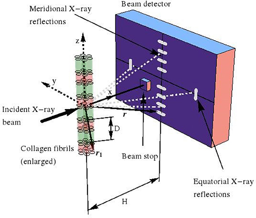
Figure 1. Small angle X-ray scattering (SAXS) device, used for investigation of fibrillar collagen structures.

Moreover, when considering that, in an X-ray diffractometer, the scattered pattern is recorded on a detector which is located some tens to hundreds of centimeters away from the (nano-to-micrometer sized) sample acting as the scattering source, the far-field approximation—also known as Fraunhofer diffraction [64]—is valid and reads as:

$\begin{array}{cc}\begin{array}{l}\frac{\left|{\text{r}}_1\right|}{\left|\text{r}\right|}\ll 1\end{array}& (18)\end{array}$

whereby the location vectors r₁ and r now label positions inside the sample and on the detector, respectively, see Figure 1 for a typical SAXS device. In order to obtain the scattered electromagnetic wave resulting from the collision of the harmonic incident wave (13) and (14), with the charged object filling volume V, we replace, in Equation (13), r by r₁, and t by (t − |r − r₁|/c). We insert the corresponding result into Equation (12), which yields Equation (S10). Then, after a series of approximation steps, given through (S11–S16), we arrive at

$\begin{array}{cc}\begin{array}{l}\text{E}(\text{r},t)=\frac{exp\left(-i\omega \left(t-\frac{\left|\text{r}\right|}{c}\right)\right)}{4\pi \left|\text{r}\right|{\omega }^2{ϵ}_0}\left|{\text{k}}_0{|}^2\right|{\text{E}}_0|\\ \times {\displaystyle \underset{V}{\int }}\frac{{\rho }_e^2}{{\rho }_m}({\text{r}}_1)exp(-i\Delta \text{k}.{\text{r}}_1)d^3{\text{r}}_1\end{array}& (19)\end{array}$

inducing Δk as the deviation of the scattered wave vector from its incident counterpart, which mathematically reads as

$\begin{array}{cc}\begin{array}{l}\Delta \text{k}=\text{k}-{\text{k}}_0=k_0\left(\frac{\text{r}}{\left|\text{r}\right|}-\frac{{\text{k}}_0}{k_0}\right)=\Delta k_x{\text{e}}_x+\Delta k_y{\text{e}}_y+\Delta k_z{\text{e}}_z\\ =k_0\left[(sin\theta cos\Phi -1){\text{e}}_x+(sin\theta sin\Phi ){\text{e}}_y+cos\theta {\text{e}}_z\right]\end{array}& (20)\end{array}$

where the definition of Euler angles Φ and θ follows from Figure 2. For an experimental setup related to the small angle X-ray scattering, sin θ cos Φ ≈ 1, so that Δk reduces to

$\begin{array}{cc}\begin{array}{l}\Delta \text{k}=\Delta k_y{\text{e}}_y+\Delta k_z{\text{e}}_z\end{array}& (21)\end{array}$

and the latter components (or their values divided by 2π, S_i = Δk_i/(2π)) are standardly reported in the literature, see e.g., Chen et al. [58].

FIGURE 2

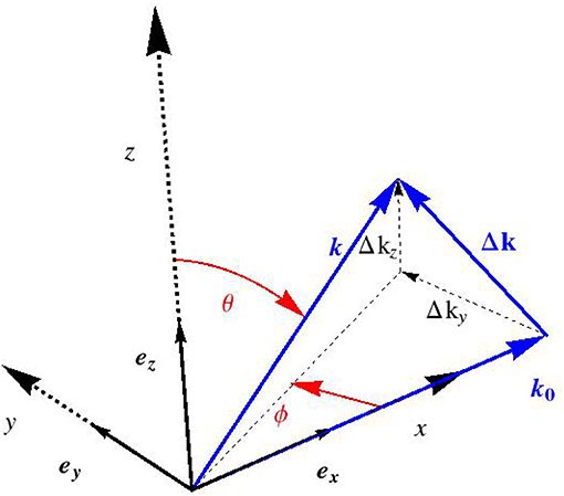
Figure 2. Scattering vector Δk in Cartesian coordinate systems (x, y, z) fixed to the sample.

Moreover, X-ray scattering experiments normally do not provide access to the electric field of the scattered waves, but rather to their intensity field, called scattering pattern. The intensity I is defined as the average over many periods of the Poynting vector S, which, in turn, is defined as

$\begin{array}{cc}\begin{array}{l}\text{S}=\frac{1}{{\mu }_0}\text{E}\times \text{B}\end{array}& (22)\end{array}$

Hence, the mathematical expression for the intensity reads as

$\begin{array}{cc}\begin{array}{l}I=\left|\langle \text{S}\rangle \right|=\frac{1}{2{\mu }_0}{R}(\text{E}\times {\text{B}}^{*})\end{array}& (23)\end{array}$

with (.)* as the complex conjugate of (complex) quantity (.), ${R}(.)$ as the real part of (complex) quantity (.), and 〈.〉 as the average over time periods. The expression for the magnetic field which corresponds to the electric field (19), is then obtained from the Maxwell-Faraday Equation (4), as

$\begin{array}{cc}\begin{array}{l}\frac{\partial \text{B}}{\partial t}=-\text{rot E}=-i{\text{k}}_0\times \text{E}\Rightarrow \text{B}=\frac{1}{\omega }{\text{k}}_0\times \text{E}\end{array}& (24)\end{array}$

Insertion of Equations (24) and (19), into (23) finally provides access to the scattered intensity patterns in the format

$\begin{array}{cc}\begin{array}{l}I(\Delta \text{k})=\frac{1}{2{\mu }_0}{\left(\frac{1}{4\pi \left|\text{r}\right|{\omega }^2}\right)}^2\left|{\text{k}}_0{|}^4\right|{\text{E}}_0{|}^2\frac{\left|{\text{k}}_0\right|}{{ϵ}_0^2\omega }\\ \times {\left[{\displaystyle {\int }_V}\frac{{\rho }_e^2}{{\rho }_m}({\text{r}}_1)exp(-i\Delta \text{k}.{\text{r}}_1)d^3{\text{r}}_1\right]}^2\end{array}& (25)\end{array}$

The intensity of the scattered wave can be decomposed into the product of the intensity I₀ scattered by an electron situated at the origin, and the square of the amplitude A of the electromagnetic wave, according to

$\begin{array}{cc}\begin{array}{l}I=I_{0}A(\Delta \text{k})A^{*}(\Delta \text{k})\end{array}& (26)\end{array}$

where I₀ reads as

$\begin{array}{cc}\begin{array}{l}{I}_0=\frac{1}{2{\mu }_0{c}^5}{\left(\frac{\left|{\text{E}}_0\right|}{4\pi \left|\text{r}\right|{ϵ}_0}\right)}^2\end{array}& (27)\end{array}$

and where the amplitude of the scattered wave A (Δk) is given by

$\begin{array}{cc}\begin{array}{l}A(\Delta \text{k})={\displaystyle {\int }_V}\frac{{\rho }_e^2}{{\rho }_m}({\text{r}}_1)exp(-i\Delta \text{k}.{\text{r}}_1)d^3{\text{r}}_1\\ =\frac{e}{{M}}{\displaystyle {\int }_V}{\rho }_e({\text{r}}_1)exp(-i\Delta \text{k}.{\text{r}}_1)d^3{\text{r}}_1\end{array}& (28)\end{array}$

with e ≈ 1.6021 × 10⁻¹⁹C as the elementary charge and ${M}\approx 9.1093\times 10^{-31}\mathrm{\text{ kg}}$ as the mass of one electron. Expressions (26–28) are usually considered as the starting point for X-ray pattern computations. Hence, it is the electron density distribution for a given tissue, which is the only input needed for computation of the diffraction pattern. It will be quantified in section 2.3.

2.3. Key Organizational Characteristics of Bone Ultrastructure

As shown in a series of contributions [37, 40–42, 65], two key characteristics of bone ultrastructure have been mandatory for successfully upscaling the material's elastic, cohesive, frictional, and viscous properties, from the “universal” elastic, cohesive, frictional, and viscous properties of bone's nanoscaled elementary components; i.e., of hydroxyapatite mineral, of collagen, and of water with non-collageneous organic matter. These characteristics are:

(i) the average extrafibrillar mineral concentration equals the average extracollageneous mineral concentration throughout the entire (i.e., extrafibrillar and fibrillar) ultrastructural compartment under investigation [36, 66];

(ii) the collagen fibrils are parallel to each other, but are randomly distributed both along the axial tissue direction and throughout the equatorial plane, i.e., the plane orthogonal to the fibrillar orientation [37, 42].

Characteristic (i) will be the basis for quantifying the electron density distributions throughout bone ultrastructure in sections 2.4 and 2.5, and characteristic (ii) will play a key role for mathematically re-constructing the organization of collagen molecules and fibrils, as described in section 2.6.

2.4. Electron Densities in the Extrafibrillar Space

As explained by Lees [67], mineralization of the osteoid, i.e., the unmineralized organic matrix laid down by osteoblasts [68, 69], is related to precipitation of hydroxyapatite mineral with a real mass density of ${\rho }_{m,HA}=3{\mathrm{\text{g/cm}}}^3$ [3], out of an aqueous solution with a mass density close to that of water, ${\rho }_{m,fl}=1{\mathrm{\text{g/cm}}}^3$. This implies mineralization-induced shrinkage of the bone tissue with respect to the unmineralized state of osteoid. Tissue volume changes are associated to changes in the X-ray or neutron diffraction spacings d_w. The latter reflect the lateral distances between the 1nm thick collagen molecules which make up larger organizational units called fibrils, with tens to hundreds of nanometers in diameter and up to several microns in length [70–73]. In accordance with the aforementioned mineralization-induced tissue shrinkage, the maximum spacings of $d_w^0=1.52\mathrm{\text{nm}}$ are encountered in unmineralized tissues, and values around d_w ≈ 1.25nm are typical for mineralized bone tissue, see e.g., Lees et al. [1], Bonar et al. [2], and Lees and Mook [74] for a collection of respective experimental data.

Setting the aforementioned precipitation process into a closed thermodynamic setting, Morin and Hellmich [66] provided the following relationship for the diffraction spacing in mineralized tissues

$\begin{array}{cc}\begin{array}{l}{d}_w=d_w^0\sqrt{\frac{1-f_{ef}^0\times \left[1-({\rho }_{m,HA}/{\rho }_{m,fl}-1)\times f_{HA}^{ec}\times \frac{f_{col}^{ec}}{{\rho }_{m,HA}{f}_{HA}^{ec}/{\rho }_{m,fl}+f_{fl}^{ec}}\right]}{(1-f_{ef}^0)\times \left[1+({\rho }_{m,HA}/{\rho }_{m,fl}-1)\times f_{HA}^{ec}\right]}}\end{array}& (29)\end{array}$

where $f_{col}^{ec}$, $f_{HA}^{ec}$, and $f_{fl}^{ec}$ denote the volume fractions of collagen, mineral, and fluid per volume of extracellular bone matrix. From an extensive collection of experimental data [65, 75], these volume fractions have been shown to be fully governed by the mass density of the extracellular bone tissue, ρ_m,ec; through the following relations

$\begin{array}{cc}\begin{array}{l}\text{if }{\rho }_{m,ec}\le 1.978{\text{ g/cm}}^3\{\begin{array}{l}{f}_{HA,ec}({\rho }_{m,ec})=\frac{1}{{\rho }_{m,HA}}(1.328{\rho }_{m,ec}-1.394),\hfill \\ f_{org,ec}({\rho }_{m,ec})=\frac{1}{{\rho }_{m,org}}(0.389{\rho }_{m,ec}-0.239),\hfill \\ f_{H_{2}O,ec}({\rho }_{m,ec})=1-f_{HA,ec}-f_{org,ec}.\hfill \end{array}\\ \text{if }{\rho }_{m,ec}\ge 1.978{\text{ g/cm}}^3\{\begin{array}{l}{f}_{HA,ec}({\rho }_{m,ec})=\frac{1}{{\rho }_{m,HA}}(1.730{\rho }_{m,ec}-2.190),\hfill \\ f_{org,ec}({\rho }_{m,ec})=\frac{1}{{\rho }_{m,org}}(-0.518{\rho }_{m,ec}+1.554),\hfill \\ f_{H_{2}O,ec}({\rho }_{m,ec})=1-f_{HA,ec}-f_{org,ec}.\hfill \end{array}\end{array}& (30)\end{array}$

with ρ_m,org = 1.42 g/cm³ [3] as the mass density of the organic matter.

As 90% of the organic matter in bone is collagen [76], the extracellular volume fraction of collagen follows as

$\begin{array}{cc}\begin{array}{l}{f}_{col}^{ec}=0.9f_{org}^{ec}\end{array}& (31)\end{array}$

Moreover, $f_{ef}^0$ in Equation (29) denotes the volume fraction of the extrafibrillar space in unmineralized tissue, reading as [66]

$\begin{array}{cc}\begin{array}{l}{f}_{ef}^0=1-\frac{1}{0.88}{\left(\frac{d_w^0}{d_{dry}}\right)}^2\frac{f_{col}^{ec}({\rho }_{m,ec})}{\frac{{\rho }_{m,HA}}{{\rho }_{m,fl}}{f}_{HA}^{ec}({\rho }_{m,ec})+f_{fl}^{ec}({\rho }_{m,ec})+f_{col}^{ec}({\rho }_{m,ec})}\end{array}& (32)\end{array}$

with d_dry = 1.09nm [1, 67] as the minimum diffraction spacing occurring in fully dried unmineralized collageneous tissues. According to the standard geometrical notions of continuum mechanics [77, 78], the diffraction spacing gives access to the ratio between the hydrated and the fully dried fibrillar volumes, through

$\begin{array}{cc}\begin{array}{l}\frac{V_{fib}}{V_{dry}}={\left(\frac{d_w}{d_{dry}}\right)}^2\end{array}& (33)\end{array}$

which, in turn, allows for quantification of the fibrillar volume fraction through

$\begin{array}{cc}\begin{array}{l}{f}_{fib}^{ec}=\frac{V_{fib}}{V^{ec}}=\frac{V_{fib}}{V_{dry}}\frac{V_{dry}}{V_{col}}\frac{V_{col}}{V^{ec}}=\frac{f_{col}^{ec}}{0.88}{\left(\frac{d_w}{d_{dry}}\right)}^2\end{array}& (34)\end{array}$

as it is known that fully hydrated collageneous tissue contains zero extrafibrillar space, and 12% intermolecular porosity, while the remaining 88% are filled up by molecular collagen [78, 79], which implies that

$\begin{array}{cc}\begin{array}{l}{V}_{col}=0.88V_{dry}\end{array}& (35)\end{array}$

The equivalence of apparent mineral density in the extrafibrillar and extracollageneous fibrillar space, as shown by Hellmich and Ulm [36], implies the following expression for the relative fraction of hydroxyapatite in the extrafibrillar space

$\begin{array}{cc}\begin{array}{l}{\varphi }_{HA,ef}=\frac{1-f_{fib}^{ec}}{1-f_{col}^{ec}}\end{array}& (36)\end{array}$

which, in turn, provides access to the volume fractions of mineral in the fibrillar and extrafibrillar spaces, respectively

$\begin{array}{cc}\begin{array}{l}{f}_{HA}^{fib}=\frac{f_{HA}^{ec}(1-{\varphi }_{HA,ef})}{f_{fib}^{ec}}\end{array}& (37)\end{array}$

$\begin{array}{cc}\begin{array}{l}{f}_{HA}^{ef}=\frac{f_{HA}^{ec}{\varphi }_{HA,ef}}{f_{ef}^{ec}}\end{array}& (38)\end{array}$

The latter volume fraction provides direct access to the electron density found in the extrafibrillar space, according to the integration rule for extensive physical quantities, reading for the extrafibrillar electron density as

$\begin{array}{cc}\begin{array}{l}{\rho }_{e,ef}={\rho }_{e,HA}{f}_{HA}^{ef}+{\rho }_{e,H_{2}O}(1-f_{HA}^{ef})\end{array}& (39)\end{array}$

whereby the electron densities of hydroxyapatite and water amount to ${\rho }_{e,HA}=940{\mathrm{\text{e/nm}}}^3$ and ${\rho }_{e,H_{2}O}=330{\text{e}/\text{nm}}^3$ [80], respectively.

2.5. Electron Densities in the Intra-Fibrillar Gap and Overlap Zones

The determination of the electron densities in the fibrillar space requires consideration of the D-periodic structure of the so-called gap and overlap zones, as discovered by Hodge and Petruska [81]. The lengths of these zones are quantified as D_gap = 0.52D and D_OV = 0.47D, with D = 67nm as the so-called macroperiod of collagen [82]. The average electron densities in the aforementioned gap and overlap zones can be computed from

$\begin{array}{cc}\begin{array}{l}{\rho }_{e,gap}={\rho }_{e,HA}{f}_{HA}^{gap}+{\rho }_{e,col}{f}_{col}^{gap}+{\rho }_{e,H_{2}O}{f}_{H_{2}O}^{gap}\end{array}& (40)\end{array}$

$\begin{array}{cc}\begin{array}{l}{\rho }_{e,OV}={\rho }_{e,HA}{f}_{HA}^{OV}+{\rho }_{e,col}{f}_{col}^{OV}+{\rho }_{e,H_{2}O}{f}_{H_{2}O}^{OV}\end{array}& (41)\end{array}$

whereby the electron density of collagen amounts to ${\rho }_{e,col}=450\text{ e}/\text{n}{\text{m}}^3$ [80]; and $f_{HA}^{gap}$, $f_{HA}^{OV}$, $f_{col}^{gap}$, $f_{col}^{OV}$, $f_{H_{2}O}^{gap}$, and $f_{H_{2}O}^{OV}$ are the volume fractions of hydroxyapatite, collagen, and water per volume of gap zone and overlap zone, respectively.

We will now express the latter volume fractions in terms of macroperiod D and diffraction spacing d. Thereby, we start with the collagen volume fractions $f_{col}^{gap}$ and $f_{col}^{OV}$, and we introduce associated volumes found within a representative piece of bone ultrastructure, namely the volumes occupied by gap zones, by fibrils, and by collagen, respectively; denoted as V_gap, V_fib, and V_col. Furthermore, we introduce the volume of collagen within gap zone volume as $V_{col}^{gap}$. In terms of these volume quantities, the volume fractions of collagen per gap and overlap zone readily read as

$\begin{array}{cc}\begin{array}{l}{f}_{col}^{gap}=\frac{V_{col}^{gap}}{V_{gap}}=\frac{V_{col}^{gap}}{V_{col}}\frac{V_{fib}}{V_{gap}}\frac{V_{col}}{V_{fib}}=\frac{V_{col}^{gap}}{V_{col}^{gap}+V_{col}^{OV}}\frac{V_{fib}}{V_{gap}}\frac{V_{col}}{V_{fib}}\end{array}& (42)\end{array}$

$\begin{array}{cc}\begin{array}{l}{f}_{col}^{OV}=\frac{V_{col}^{OV}}{V^{OV}}=\frac{V_{col}^{OV}}{V_{col}}\frac{V_{fib}}{V_{OV}}\frac{V_{col}}{V_{fib}}=\frac{V_{col}^{OV}}{V_{col}^{gap}+V_{col}^{OV}}\frac{V_{fib}}{V_{OV}}\frac{V_{col}}{V_{fib}}\end{array}& (43)\end{array}$

Given the cylindrical shape of the fibrils, the volume fractions per fibrillar space, of the gap and the overlap zones, are in the same ratio as the lengths of these zones, which implies the following relations

$\begin{array}{cc}\begin{array}{l}\frac{V_{gap}}{V_{fib}}=\frac{D_{gap}}{D}=0.53\iff V_{gap}=V_{fib}\frac{D_{gap}}{D}=0.53V_{fib}\end{array}& (44)\end{array}$

$\begin{array}{cc}\begin{array}{l}\frac{V_{OV}}{V_{fib}}=\frac{D_{OV}}{D}=0.47\iff V_{gap}=V_{fib}\frac{D_{OV}}{D}=0.47V_{fib}\end{array}& (45)\end{array}$

Comprehensive diffraction data on unmineralized collagen can be satisfactorily represented through a pentameric scheme called five-stranded microfibril model [83–86], whereby the (chemical) concentrations of molecular collagen in gap and overlap zones are in a ratio of four to five. This implies the following relationship for the volumes of molecular collagen in the gap and overlap zones, respectively,

$\begin{array}{cc}\begin{array}{l}\frac{V_{col}^{gap}}{V_{col}^{OV}}=0.8\frac{D_{gap}}{D_{OV}}\end{array}& (46)\end{array}$

Finally, insertion of (33), (35), (44)₁, (45)₁, and (46), into (42) and (43) yields the desired relations between the experimentally available quantities d_dry, d_w, D_gap, D_OV, and D on the one hand, and the collagen volume fractions in the gap and overlap zones, on the other hand. Mathematically, they read as

$\begin{array}{cc}\begin{array}{l}{f}_{col}^{gap}=\frac{0.8D_{gap}}{D_{OV}+0.8D_{gap}}\frac{D}{D_{gap}}0.88{\left(\frac{d_{dry}}{d_w}\right)}^2\end{array}& (47)\end{array}$

$\begin{array}{cc}\begin{array}{l}{f}_{col}^{OV}=\frac{D_{OV}}{D_{OV}+0.8D_{gap}}\frac{D}{D_{OV}}0.88{\left(\frac{d_{dry}}{d_w}\right)}^2\end{array}& (48)\end{array}$

Next, we turn toward the volume fractions of mineral in the gap and overlap zones. We introduce additional volumes within a representative piece of bone ultrastructure, namely the volumes of mineral within the fibrils, within the gap, and within the overlap zones, respectively, denoted as $V_{HA}^{fib}$, $V_{HA}^{gap}$, and $V_{HA}^{OV}$. In terms of these as well as of the aforementioned volumes, the volume fractions of mineral in the gap and overlap zones can be expressed as

$\begin{array}{cc}\begin{array}{l}{f}_{HA}^{gap}=\frac{V_{HA}^{gap}}{V_{gap}}=\frac{V_{HA}^{gap}}{V_{HA}^{fib}}\frac{V_{fib}}{V_{gap}}\frac{V_{HA}^{fib}}{V_{fib}}=\frac{V_{HA}^{gap}}{V_{HA}^{gap}+V_{HA}^{OV}}\frac{V_{fib}}{V_{gap}}\frac{V_{HA}^{fib}}{V_{fib}}\end{array}& (49)\end{array}$

$\begin{array}{cc}\begin{array}{l}{f}_{HA}^{OV}=\frac{V_{HA}^{OV}}{V_{OV}}=\frac{V_{HA}^{OV}}{V_{HA}^{fib}}\frac{V_{fib}}{V_{OV}}\frac{V_{HA}^{fib}}{V_{fib}}=\frac{V_{HA}^{OV}}{V_{HA}^{gap}+V_{HA}^{OV}}\frac{V_{fib}}{V_{OV}}\frac{V_{HA}^{fib}}{V_{fib}}\end{array}& (50)\end{array}$

In order to link these volumes to actually measurable quantities, we consider that the on-average mineral concentration in the extracollageneous compartments of bone ultrastructure is uniform, as evidenced by Hellmich and Ulm [36], which implies the identity of the extracollageneous mineral concentrations in the gap and overlap zones as well. Mathematically, this reads as

$\begin{array}{cc}\begin{array}{l}\frac{M_{HA}^{gap}}{V_{gap}-V_{col}^{gap}}=\frac{M_{HA}^{OV}}{V_{OV}-V_{col}^{OV}}\end{array}& (51)\end{array}$

It is helpful to transform (51) into a mass ratio,

$\begin{array}{cc}\begin{array}{l}\frac{M_{HA}^{gap}}{M_{HA}^{OV}}=\frac{{\rho }_{m,HA}{V}_{HA}^{gap}}{{\rho }_{m,HA}{V}_{HA}^{OV}}=\frac{V_{gap}-V_{col}^{gap}}{V_{OV}-V_{col}^{OV}}\end{array}& (52)\end{array}$

Subsequent insertion of (44)₂ and (45)₂ into (52) yields

$\begin{array}{cc}\begin{array}{l}\frac{V_{HA}^{gap}}{V_{HA}^{OV}}=\frac{\frac{D_{gap}}{D}{V}_{fib}-\frac{0.8D_{gap}}{D_{OV}+0.8D_{gap}}{V}_{col}}{\frac{D_{OV}}{D}{V}_{fib}-\frac{D_{OV}}{D_{OV}+0.8D_{gap}}{V}_{col}}\\ =\frac{D_{gap}\left[(D_{OV}+0.8D_{gap})-0.8D0.88{\left(\frac{d_{dry}}{d_w}\right)}^2\right]}{D_{OV}\left[(D_{OV}+0.8D_{gap})-D0.88{\left(\frac{d_{dry}}{d_w}\right)}^2\right]}\\ =g_{HA}\frac{D_{gap}}{D_{OV}}\end{array}& (53)\end{array}$

whereby the abbreviation g_HA stands for

$\begin{array}{cc}\begin{array}{l}{g}_{HA}=\frac{\left[(D_{OV}+0.8D_{gap})-0.8D0.88{\left(\frac{d_{dry}}{d_w}\right)}^2\right]}{\left[(D_{OV}+0.8D_{gap})-D0.88{\left(\frac{d_{dry}}{d_w}\right)}^2\right]}\end{array}& (54)\end{array}$

Insertion of (53) and (54), as well as of (44)₁ and (45)₁, into (49) and (50) yields the mineral volume fractions per gap and overlap zones, as functions of D, D_gap, D_OV, and d_w. Mathematically, they read as

$\begin{array}{cc}\begin{array}{l}{f}_{HA}^{gap}=\frac{g_{HA}(d_w)D_{gap}}{D_{OV}+g_{HA}(d_w)D_{gap}}\frac{D}{D_{gap}}{f}_{HA}^{fib}\end{array}& (55)\end{array}$

$\begin{array}{cc}\begin{array}{l}{f}_{HA}^{OV}=\frac{D_{OV}}{D_{OV}+g_{HA}(d_w)D_{gap}}\frac{D}{D_{OV}}{f}_{HA}^{fib}\end{array}& (56)\end{array}$

The remaining volumes of the gap and overlap zones are filled with water, with the corresponding volume fractions reading as

$\begin{array}{cc}\begin{array}{l}{f}_{H_{2}O}^{gap}=1-f_{HA}^{gap}-f_{col}^{gap}\end{array}& (57)\end{array}$

$\begin{array}{cc}\begin{array}{l}{f}_{H_{2}O}^{OV}=1-f_{HA}^{OV}-f_{col}^{OV}\end{array}& (58)\end{array}$

Conclusively, the average electron density in the gap and overlap zone can be computed by substituting (42), (43), (49), (50), (57), and (58), into (40) and (41), respectively, yielding

$\begin{array}{cc}\begin{array}{l}{\rho }_{e,gap}={\rho }_{e,HA}\frac{g_{HA}(d_w)D}{D_{OV}+g_{HA}(d_w)D_{gap}}{f}_{HA}^{fib}\\ +{\rho }_{e,col}\frac{0.8D}{D_{OV}+0.8D_{gap}}0.88{\left(\frac{d_{dry}}{d_w}\right)}^2\\ +{\rho }_{e,H_{2}O}(1-\frac{g_{HA}(d_w)D}{D_{OV}+g_{HA}(d_w)D_{gap}}{f}_{HA}^{fib}\\ -\frac{0.8D}{D_{OV}+0.8D_{gap}}0.88{\left(\frac{d_{dry}}{d_w}\right)}^2)\end{array}& (59)\end{array}$

$\begin{array}{cc}\begin{array}{l}{\rho }_{e,OV}={\rho }_{e,HA}\frac{D}{D_{OV}+g_{HA}(d_w)D_{gap}}{f}_{HA}^{fib}\\ +{\rho }_{e,col}\frac{D}{D_{OV}+0.8D_{gap}}0.88{\left(\frac{d_{dry}}{d_w}\right)}^2\\ +{\rho }_{e,H_{2}O}(1-\frac{D}{D_{OV}+g_{HA}(d_w)D_{gap}}{f}_{HA}^{fib}\\ -\frac{D}{D_{OV}+0.8D_{gap}}0.88{\left(\frac{d_{dry}}{d_w}\right)}^2)\end{array}& (60)\end{array}$

2.6. Organizational Patterns of Fibrils

Evaluation of Equation (28) requires not only the knowledge of electron densities, as quantified in the last two subsections, but also some essential information on the spatial organization of fibrils throughout the bone ultrastructure. Starting with a hexagonal arrangement of fibrils in the transverse plane [87], see Figure 3, the distance d_fib between fibrils can be determined from the radius of the fibrils, R_fib ≈ 40nm [70–72], and from the volume fraction of fibrils, $f_{fib}^{ec}$, as introduced in Equation (34). The corresponding mathematical relation reads as

$\begin{array}{cc}\begin{array}{l}{f}_{fib}^{ec}=\frac{V_{fib}}{V_{ec}}=\frac{\pi R_{fib}^2}{{(d_{fib})}^2\sqrt{3}/2}\Rightarrow d_{fib}=\sqrt{\frac{2\sqrt{3}\pi R_{fib}^2}{3f_{fib}^{ec}}}\end{array}& (61)\end{array}$

FIGURE 3

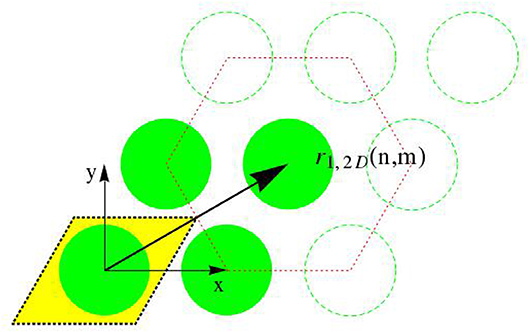
Figure 3. Illustration of a hexagonal lattice and unit cell.

Accordingly, the center points of the transverse sections through the fibrils form a hexagonal lattice, and we distribute such lattices at periods D along the z-direction. All points created in that way are identified through the following set of location vectors r₁

$\begin{array}{cc}\begin{array}{l}{\text{r}}_1^{m,n,o}=d_{fib}\left((m+\frac{n}{2}{\text{e}}_x)+\frac{\sqrt{3}n}{2}{\text{e}}_y\right)+oD{\text{e}}_z\end{array}& (62)\end{array}$

with integers m ∈ [−m_max/2, m_max/2 − 1], n ∈ [−n_max/2, n_max/2 − 1], and o = 0, 1, …., N_period − 1, so that the number of fibrils follows as n_fib = m_max × n_max. The position function collecting all these points, i.e., the function vanishing anywhere else, is given through

$\begin{array}{cc}\begin{array}{l}p({\text{r}}_1)=p(x,y,z)={\displaystyle \sum _{m=-m_{max}/2}^{m_{max}/2-1}}{\displaystyle \sum _{n=-n_{max}/2}^{n_{max}/2-1}}\delta \left(x-d_{fib}\left(m+\frac{n}{2}\right)\right)\\ \times \delta \left(y-d_{fib}\frac{\sqrt{3}}{2}n\right)\times {\displaystyle \sum _{o=0}^{N_{period}-1}}\delta (z-oD)\end{array}& (63)\end{array}$

whereby δ stands for the Dirac distribution; and x, y, and z are the components of location vector r₁ with respect to the base frame e_x, e_y, and e_z; so that r₁ = xe_x + ye_y + ze_z. Next, we link unit cells representing the ultrastructural organization, to the aforementioned lattice arrangement of points. The electron density distribution throughout one such unit cell is given through

$\begin{array}{cc}\begin{array}{l}{\rho }_{e,cell}(x,y,z)={\rho }_{e,ef}{\chi }_{ef}(x,y,z)+{\rho }_{e,gap}{\chi }_{gap}(x,y,z)\\ +{\rho }_{e,OV}{\chi }_{OV}(x,y,z)\\ =({\rho }_{e,ef}-{\rho }_{e,0}){\chi }_{ef}(x,y,z)+({\rho }_{e,gap}-{\rho }_{e,0}){\chi }_{gap}(x,y,z)\\ +({\rho }_{e,OV}-{\rho }_{e,0}){\chi }_{OV}(x,y,z)+{\rho }_{e,0}\end{array}& (64)\end{array}$

whereby χ_ef, χ_gap, and χ_OV are the characteristic functions of the extrafibrillar space, the gap and overlap zones, respectively; and where ρ_e,ef, ρ_e,gap, and ρ_e,OV are the electron densities of the aforementioned space and zones; ρ_e,0 stands for any uniform electron density, and can be chosen, for instance, as the uniform electron density of the extrafibrillar space: ρ_e,0 = ρ_e,ef. This choice allows for doing without characteristic function of the extrafibrillar space [88]. The characteristic functions of the gap and overlap zones are defined through

$\begin{array}{cc}\begin{array}{l}{\chi }_{gap}(x,y,z)=\left[1-\Theta (\sqrt{x^2+y^2}-R_{fib})\right]\\ \times \left[\mathrm{\text{sgn}}(z-D_{OV})-\mathrm{\text{sgn}}(z-D_{OV}-D_{gap})\right]\end{array}& (65)\end{array}$

$\begin{array}{cc}\begin{array}{l}{\chi }_{OV}(x,y,z)=\left[1-\Theta (\sqrt{x^2+y^2}-R_{fib})\right]\\ \times \left[\mathrm{\text{sgn}}(z)-\mathrm{\text{sgn}}(z-D_{OV})\right]\end{array}& (66)\end{array}$

whereby Θ stands for the Heaviside distribution and sgn stands for the signum function. In (65) and (66), the first term describes the fibril as the space contained inside a cylinder centered at the origin of the unit cell and having a radius R_fib in the transverse direction; and the second term refers to the axial position of the gap and overlap zones. Conclusively, the electron density at any point of a perfect fibrillar lattice results from a convolution product between the charge density of a unit cell ρ_e,cell and the location function of the unit cells p(r₁)

$\begin{array}{cc}\begin{array}{l}{\rho }_e({\text{r}}_1)=\left[{\rho }_{e,cell}*p\right]({\text{r}}_1)={\displaystyle {\int }_{V_{lattice}}}({\rho }_{e,cell}({\text{r}}_1^{*}))p({\text{r}}_1-{\text{r}}_1^{*})d^3{\text{r}}_1^{*}\end{array}& (67)\end{array}$

with * as the convolution product.

Combining (28) and (67) leads to the following expression of the amplitude of the scattered wave for a perfect hexagonal lattice of unit cells

$\begin{array}{cc}\begin{array}{l}{A}_{lattice}(\Delta \text{k})=\frac{e}{{M}}{\displaystyle {\int }_{V_{lattice}}}{\displaystyle {\int }_{V_{lattice}}}({\rho }_{e,cell}({\text{r}}_1^{*})-{\rho }_{e,0})\\ \times p({\text{r}}_1-{\text{r}}_1^{*})exp(-i\Delta \text{k}.{\text{r}}_1)d^3{\text{r}}_1^{*}{d}^3{\text{r}}_1\end{array}& (68)\end{array}$

which can be interpreted as the Fourier transform ${F}$ of the electron density distribution through the hexagonal lattice. An assembly of numerous such lattices with different orientations in the transverse plane are considered to be representative of the overall bone ultrastructure. The corresponding amplitudes of the scattered waves arising from the bone ultrastructure, A_ec, are obtained as the sum of n_orient subvolumes of perfect hexagonal lattices with different transversal orientations. Mathematically, this reads as

$\begin{array}{cc}\begin{array}{l}{A}_{ec}(\Delta \text{k})=\frac{e}{{M}}{\displaystyle {\int }_{V_{lattice}}}{\displaystyle {\int }_{V_{lattice}}}{\displaystyle \sum _{q=1}^{n_{orient}}}({\rho }_{e,cell}({\text{r}}_1^{*})-{\rho }_{e,0})\\ \times p_q({\text{r}}_1-{\text{r}}_1^{*})exp(-i\Delta \text{k}.{\text{r}}_1)d^3{\text{r}}_1^{*}{d}^3{\text{r}}_1\end{array}& (69)\end{array}$

with new position function p_q denoting the position function for a lattice rotated by an angle Ψ_q with respect to the lattice with position function (63). This new position function p_q mathematically reads as

$\begin{array}{cc}\begin{array}{l}{p}_q(r_1)=p_q(x,y,z)\\ ={\displaystyle \sum _{m=-m_{max}/2}^{m_{max}/2-1}{\displaystyle \sum _{n=-n_{max}/2}^{n_{max}/2-1}\delta }}(x-d_{fib}(\left(m+\frac{n}{2}\right)\cos {\text{ Ψ}}_q\\ +\frac{\sqrt{3}n}{2}\sin {\text{ Ψ}}_q))\\ \times \delta \left(y-d_{fib}\left(-\left(m+\frac{n}{2}\right)\sin {\text{ Ψ}}_q+\frac{\sqrt{3}n}{2}\cos {\text{ Ψ}}_q\right)\right)\\ \times {\displaystyle \sum _{o=0}^{N_{period}-1}\delta }\left(z-oD\right)\end{array}& (70)\end{array}$

Insertion of (64–66), and of (70), into (69), while taking into account the components of the scattering vector (21) as well as the properties of the Fourier transform given through (S17–S29), yields the amplitude of the wave vectors resulting from scattering of X-ray beams transgressing a sample of bone ultrastructure, as

$\begin{array}{cc}\begin{array}{l}{A}_{ec}(\Delta k_y,\Delta k_z)={\displaystyle \sum _{q=1}^{n_{orient}}\frac{e}{ℳ}}\frac{\mathrm{\text{exp}}\left[-i\Delta k_z{N}_{period}D)\right]-1}{\mathrm{\text{exp}}\left(-i\Delta k_{z}D\right)-1}\\ \times \frac{2\pi R_{fib}{J}_1\left(R_{fib}\Delta k_y\right)}{\Delta k_y}\frac{2i}{\Delta k_z}\\ \times [({\rho }_{e,OV}-{\rho }_{e,ef})\left(\mathrm{\text{exp}}(-i\Delta k_z{D}_{OV})-1\right)\\ +({\rho }_{e,gap}-{\rho }_{e,ef})\left[\mathrm{\text{exp}}(-i\Delta k_{z}D)-\mathrm{\text{exp}}\left(-i\Delta k_z{D}_{OV}\right)\right]]\\ \times {\displaystyle \sum _{m=-m_{max}/2}^{m_{max}/2-1}{\displaystyle \sum _{n=-n_{max}/2}^{n_{max}/2-1}}}\text{ exp}[-i{d}_{fib}\Delta k_y(-\left(m+\frac{n}{2}\right)\\ \times \sin {\Psi }_q+\frac{\sqrt{3}n}{2}\cos {\Psi }_q)]\end{array}& (71)\end{array}$

Therefrom, the intensity of the scattered waves follows from Equation (26), yielding

$\begin{array}{cc}\begin{array}{l}{I}_{ec}=I_0|A_{ec}{|}^2\end{array}& (72)\end{array}$

2.7. Imperfections

Actual bone ultrastructure typically deviates from the perfect organization introduced in the previous section. Respective random features concern

(i) the axial organization where the fibrils are randomly shifted, which leads to substitutional disorder as seen in Figures 4C,D, as opposed to perfect order as seen in Figures 4A,B;

(ii) the transverse organization where the fibrils deviate from the perfect hexagonal lattice as seen in Figure 6;

(iii) the fibrillar diameters which fluctuate around a mean value.

FIGURE 4

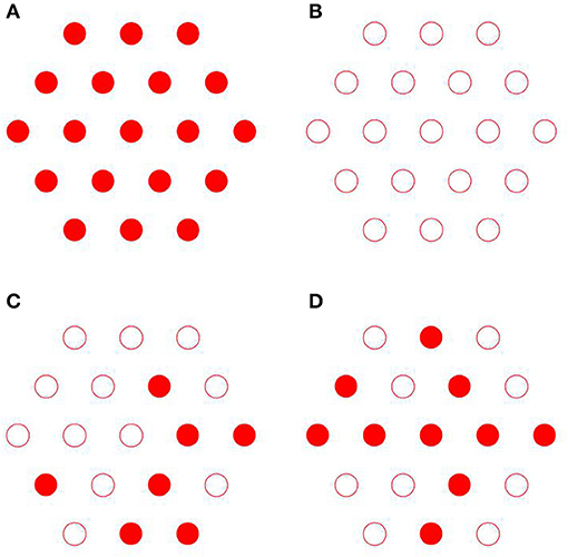
Figure 4. Hexagonal lattices cross-section without (A,B), and with (C-D) substitutional disorder.

By introducing corresponding random variables for axial shift, transverse position deviations, and fibrillar radii, denoted as $z_{m,n}^{random}$, $d_{fib,(m,n)}^{random}$, and $R_{fib,(m,n)}^{random}$, the perfect structure-related position function (63), and gap and overlap characteristic functions (65) and (66), can be extended to the following, more realistic format, as

$\begin{array}{cc}\begin{array}{l}p({\text{r}}_1)=p(x,y,z)\\ ={\displaystyle \sum _{m=-m_{max}/2}^{m_{max}/2-1}}{\displaystyle \sum _{n=-n_{max}/2}^{n_{max}/2-1}}\delta \left(x-d_{fib,(m,n)}^{random}\left(m+\frac{n}{2}\right)\right)\\ \times \delta \left(y-d_{fib,(m,n)}^{random}\frac{\sqrt{3}}{2}n\right){\displaystyle \sum _{o=0}^{N_{period}-1}}\delta \left(z-z_{m,n}^{random}-oD\right)\end{array}& (73)\end{array}$

$\begin{array}{cc}\begin{array}{l}{\chi }_{gap}(x,y,z)=\left[1-\Theta \left(\sqrt{x^2+y^2}-R_{fib,(m,n)}^{rando{m}^2}\right)\right]\\ \times \left[\mathrm{\text{sgn}}(z-D_{OV})-\mathrm{\text{sgn}}(z-D_{OV}-D^{gap})\right]\end{array}& (74)\end{array}$

$\begin{array}{cc}\begin{array}{l}{\chi }_{OV}(x,y,z)=\left[1-\Theta (\sqrt{x^2+y^2}-R_{fib,(m,n)}^{rando{m}^2})\right]\\ \times \left[\mathrm{\text{sgn}}(z)-\mathrm{\text{sgn}}(z-D_{OV})\right]\end{array}& (75)\end{array}$

In (73), $R_{fib,(m,n)}^{random}$ is a normally distributed random variable with mean value R_fib, and standard deviation σ_Rfib. In (74) and (75), $z_{m,n}^{random}$ is uniformly distributed random variable from the range [−z_max, z_max]. The corresponding scattering amplitudes arising from an imperfect lattice of differently thick fibrils with transverse as well as axial positional disorders, arise from insertion of (73–75) into (68), yielding

$\begin{array}{cc}\begin{array}{l}{A}_{lattice}(\Delta k_y,\Delta k_z)\\ ={\displaystyle \sum _{m=-m_{max}/2}^{m_{max}/2-1}{\displaystyle \sum _{n=-n_{max}/2}^{n_{max}/2-1}\frac{\mathrm{\text{exp}}\left[-i\Delta k_z{N}_{period}D\right]-1}{\mathrm{\text{exp}}\left[-i\Delta k_{z}D\right]-1}}}\\ \times \frac{2\pi R_{fib,(m,n)}^{random}{J}_1\left(R_{fib,(m,n)}^{random}\Delta k_y\right)}{\Delta k_y}\frac{2i}{\Delta k_z}\\ \times [({\rho }_{e,OV}-{\rho }_{e,ef})\left(\mathrm{\text{exp}}(-i\Delta k_z{D}_{OV})-1\right)\\ +({\rho }_{e,gap}-{\rho }_{e,ef})\left[\mathrm{\text{exp}}(-i\Delta k_{z}D)-\mathrm{\text{exp}}\left(-i\Delta k_z{D}_{OV}\right)\right]]\\ \times \mathrm{\text{exp}}\left[-i\Delta k_z{z}_{m,n}^{random}\right]\mathrm{\text{exp}}\left[-i{d}_{fib,(m,n)}^{random}\Delta k_y\frac{\sqrt{3}}{2}n\right]\end{array}& (76)\end{array}$

Some additional comments concerning the random variable $d_{fib}^{random}$ are due. In fact, the lattice disorder is introduced here in the framework of the so-called paracrystalline model [89–91]. To begin with, we consider a one-dimensional paracrystal in the transverse plane, i.e., a linear periodic lattice that is distorted in two dimensions around an axis which we denote by x^m, as depicted in Figure 5. The N lattice points defining the configuration of this one-dimensional paracrystal are given by the position vectors r^m, in the format

$\begin{array}{cc}\begin{array}{l}{\text{r}}^m={\text{r}}^{m-1}+{\text{d}}^m,\text{ for }m=0,\dots ,N-1\end{array}& (77)\end{array}$

FIGURE 5

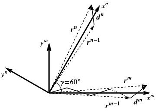
Figure 5. 1D paracrystal in initial and rotated positions.

with r₀ = d₀ = 0, and d^m being vectors with components having the following random variable characteristics:

• the mean of the x-component is $d_x^m=d_{fib}$;

• the mean of the y-component is $d_y^m=0$;

and these two random variables are jointly normal, so that their probability density distribution function reads as [92]

$\begin{array}{cc}\begin{array}{l}p(d_x^m,d_y^m)=\frac{1}{2\pi {\sigma }_x{\sigma }_y{(1-{\rho }^2)}^{1/2}}\mathrm{\text{exp}}\{-\frac{1}{2(1-{\rho }^2)}[\frac{{(d_x-d_{fib})}^2}{{\sigma }_x^2}\\ -2\rho \frac{(d_x-d_{fib})d_y}{{\sigma }_x{\sigma }_y}+\frac{{(d_y)}^2}{{\sigma }_y^2}]\}\end{array}& (78)\end{array}$

where σ_x and σ_y are the standard deviations of d_x and d_y, respectively, and $\rho =\frac{\langle d_x{d}_y\rangle -\langle d_x\rangle \langle d_y\rangle }{{\sigma }_x{\sigma }_y}$ is the correlation coefficient between d_x and d_y, with 〈.〉 denoting the average over all points of the 1D paracrystalline lattice. Characteristics of the paracrystal are controlled by the parameters σ_x, σ_y, and ρ. d_x and d_y are uncorrelated, so that ρ = 0. The standard deviations σ_x and σ_y are equal and defined as

$\begin{array}{cc}\begin{array}{l}{\sigma }_x={\sigma }_y={ℰ}\frac{d_{fib}}{\sqrt{2}}\end{array}& (79)\end{array}$

where ${E}$ characterizes the amount of disorder, and is therefore called disorder parameter.

In the same manner, we define a second 1D paracrystalline lattice distorted in two dimensions around an xⁿ axis, which results from the rotation of the x^m axis by an angle of γ = 60°, see Figure 5. This leads to two one-dimensional paracrystals in the transverse plane, one oriented along the x^m axis and one around xⁿ axis; the directions of the axes x^m and xⁿ are given by the average lattice vectors a and b, see Figure 6A. The components of d_a and standard deviations of the paracrystal along the a axis, parallel and normal to this axis, are denoted as d_a, d_⊥a, σ_a and σ_⊥a, respectively; their correlation is denoted as ρ_a. The same parameters along the b axis are denoted as d_b, d_⊥b, σ_b, σ_⊥b, and their correlation is denoted as ρ_b. The position vectors of the lattice points of the two one-dimensional paracrystals are denoted by r^m and rⁿ. The position r^{m, n} of the (m, n)th point of the ideal 2D paracrystal is given by

$\begin{array}{cc}\begin{array}{l}{\text{r}}^{m,n}={\text{r}}^m+{\text{r}}^n\end{array}& (80)\end{array}$

FIGURE 6

Figure 6. Construction of hexagonal paracrystalline lattice model – parallelogram-based 2D paracrystal model (A), space of paracrystalline lattice divided into six sectors (B), lattices built up across sectors (C), hexagonal paracrystalline lattice model used in simulations (D).

This leads to the structure shown in Figure 6A, where the paracrystalline lattice is made up of parallelograms whose edges are defined by the components of one-dimensional paracrystals. In order to create a hexagonal paracrystalline lattice, six sectors are introduced within the transverse plane, see Figure 6B, and each of these sectors is built separately by the aforementioned procedure; employing different angles γ. The corresponding result is shown in Figure 6C. From the six sector structure, the 60 fibrils which are closest to the origin of the coordinate system are selected for the simulations reported in the present paper; see Figure 6D for this selection. This is how $d_{fib}^{random}$ is realized in Equations (73) and (76).

3. Results

We seek experimental validation of the electrodynamics approach of section 2 applied to bone ultrastructure represented in sections 2.3 to 2.7, based on the data provided by Chen et al. [58] for shad fish bone. Re-construction of the electron density distribution throughout such an ultrastructure is based on the mass density and configurational data given in Tables 1, 2. Based on these input values, the electrodynamic model developed here quite satisfactorily predicts the experimentally determined meridional scattering patterns reported by Chen et al. [58]; see Figure 7C for the meridional diffraction pattern, i.e., for the component Δk_z of the wave vector. The question arises to which extent the different ultrastructural features introduced in sections 2.3 to 2.7 contribute to this rather good agreement between model predictions and experimental values. Obviously, organization disorder is a very important characteristic of bone ultrastructure, as assemblies of perfect hexagonal lattices deliver unrealistic pattterns, both as concerns the meridional and equatorial directions, see Figure 8A. Variable diameters and transverse disorder alone do not help too much in this respect, see Figures 8B,C, while the very important role of the axial shift between different fibrils becomes evident from Figure 8D, showing the results based on just this one random variable while letting the other organizational patterns in their “perfect” state. Conclusively, all introduced random characteristics are essential for arriving at the suitable model predictions depicted in Figure 8E. The second question arising concerns the distribution of mineral between the fibrillar and extrafibrillar spaces within the ultrastructure. Putting all the mineral into the extrafibrillar space; i.e., $f_{fib}^{ec}=\frac{f_{col}^{ec}}{f_{col}^{fib}}=0.473$, $f_{HA}^{fib}=0$, $f_{HA}^{ef}=\frac{f_{HA}^{ec}}{f_{ef}^{ec}}=0.63$, $f_{H_{2}O}^{ef}=\frac{f_{ef}^{ec}-f_{HA}^{ec}}{f_{ef}^{ec}}=0.37$, ${\rho }_{e,ef}=714{\mathrm{\text{ e/nm}}}^3$, ${\rho }_{e,gap}=396{\mathrm{\text{ e/nm}}}^3$, ${\rho }_{e,OV}=412{\mathrm{\text{ e/nm}}}^3$; results in a diffraction pattern loosing any significant peak characteristics, see red line in Figure 7A. Putting all the mineral into the fibrils, leads to already better results, characterized by a Root-Mean-Square error of RMS = 0.23, see Figure 7B—however, this assumption is untenable from a micromechanical viewpoint, as the tissue anisotropy would be heavily overestimated; see e.g., Hellmich and Ulm [96] and Schwarz et al. [97]. The best result is obtained for the extracollageneous mineral concentration being the same inside and outside the fibrils, characterized by a Root-Mean-Square error of RMS = 0.181, see Figure 7C—and this mineral distribution also proved essential for the performance of various micromechanical models [37, 39, 40, 65].

TABLE 1

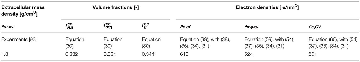
Table 1. Characteristic compositional values of the shad fish bone ultrastructure.

TABLE 2

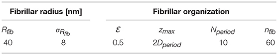
Table 2. Organizational characteristics chosen for the ultrastructure of bone; in line with observations of Parry [94].

FIGURE 7

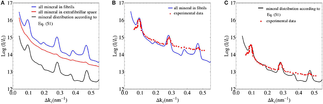
Figure 7. (A) SAXS pattern predictions based on different mineral distribution schemes in bone ultrastructure; and (B,C) comparison to experimental data of Chen et al. [58].

FIGURE 8

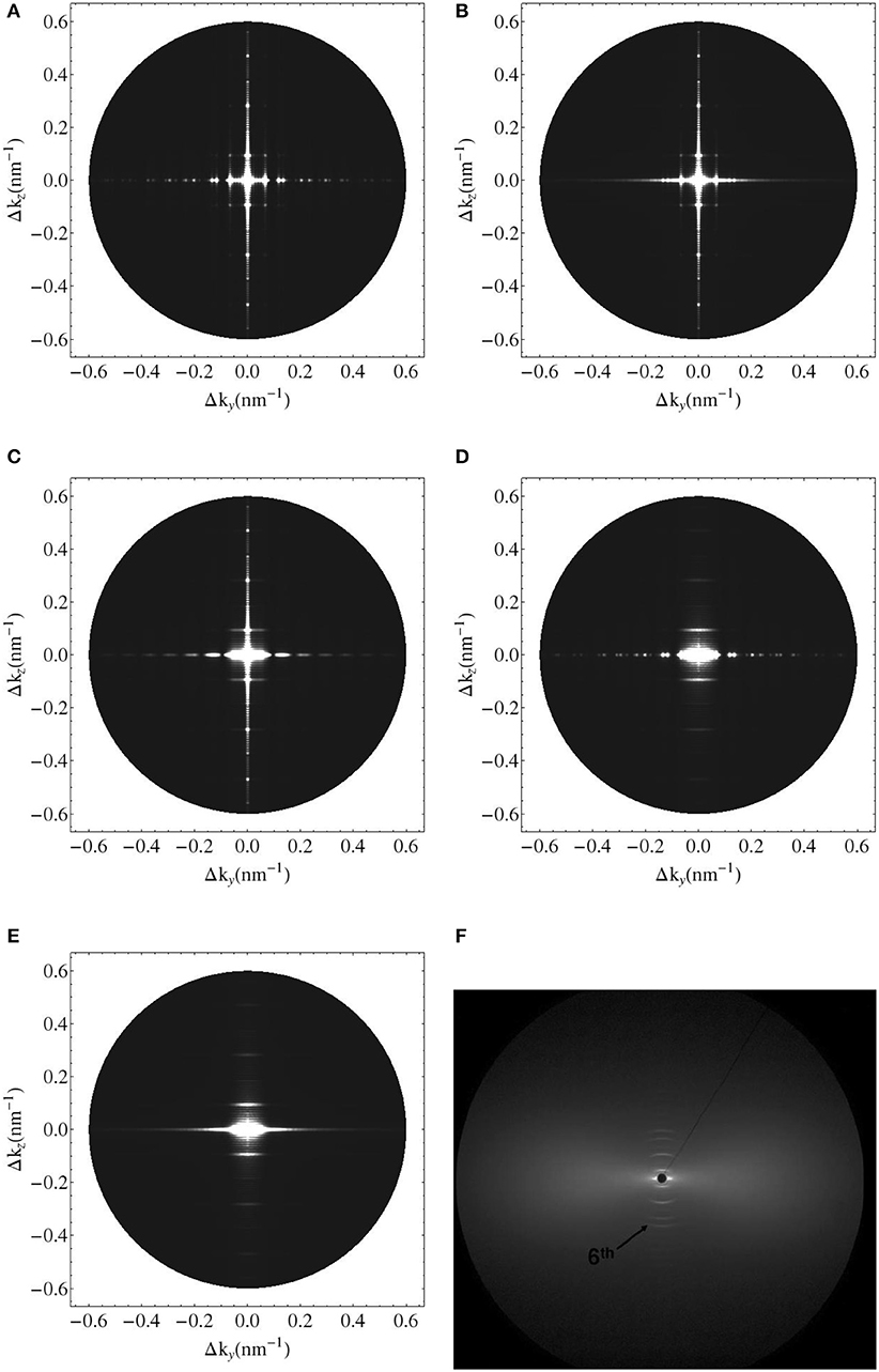
Figure 8. Simulated 2D X-ray diffraction patterns with perfect axial and hexagonal order (A), with perfect order and variable fibril diameter (B), with constant fibril diameter, perfect axial order but lattice disorder (C), with constant fibril diameter, perfect lattice order but axial disorder (D), with lattice and substitutional disorder and variable fibril diameter (E), and experimental pattern for shad fish bone (F) [95].

In the context of experimental validation of the model with regards to meridional patterns, as shown in Figure 7, the following observations are made concerning the organizational values collected into Table 2: We start with noting that changes in the mean fibrillar radius R_fib solely results in a vertical shift of the simulation curves depicted in Figure 7. As all experimental values shown there are only defined up to such a vertical shift, the mean fibrillar diameter does not enter the current model validation discussion. All other quantities given in Table 2 have only negligible effect on the model predictions depicted in Figure 7.

As a second, independent experimental check, we consider meridional scattering experiments obtained from the ulna of an adult mouse, performed by Fratzl et al. [98]. Evaluation of the equations collected into Table 1, for the extracellular mass density of mouse bone as reported by Lu et al. [99], Zhao et al. [100], and Thiagarajan et al. [101], ${\rho }_{mouse}^{ec}=1.97$ g/cm³, together with the organizational characteristics of Table 2, yields electron densities of the extrafibrilar space, and of the gap and overlap zones, respectively, as ρ_e,ef = 714 e/nm³, ρ_e,g = 560 e/nm³, ρ_e,OV = 522 e/nm³. Using the latter values for the computation of meridional scattering patterns according to Equations (39), (59), (60), and (76), yields computational predictions which agree very well with the experimentally measured SAXS patterns, see Figure 9.

FIGURE 9

Figure 9. Meridional SAXS measurements on murine bone of Fratzl et al. [98], indicated by red dots; in comparison to the model predictions based on identity of mineral concentrations in the extracollageneous and extrafibrillar spaces of bone ultrastructure, indicated by solid black line.

4. Discussion

Several contributions concerning characterization of bone tissue by means of SAXS, see e.g., Rinnerthaler et al. [102], Wess et al. [103], Grabner et al. [104], and Turunen et al. [105] and references therein, have adopted a concept put forward by Fratzl et al. [98]: The latter authors do not consider the fibrillar structure of the bone matrix, but introduce nanometer-sized crystals as the only relevant morphological feature potentially governing the shapes of the SAXS patterns. Corresponding ad hoc application of Porod's law is then suggested to deliver crystal thicknesses; and as the resulting numbers coincide with the gap zone dimensions according to the classical Hodge-Petruska model [81], the latter are proposed to lie exclusively in these elongated gap zones within a collagen matrix. This idea is obviously at odds with the comprehensive experimental evidence reviewed in the Introduction section, and beyond this observation, two additional thoughts may be noteworthy:

• From a mechanics viewpoint, this view on ultrastructural representation is very unrealistic, as can be seen from checking numbers provided by a corresponding composite model: Namely, a Mori-Tanaka scheme [106, 107] representing a contiguous matrix hosting parallel cylindrical mineral inclusions delivers by far too high ratios of longitudinal to transverse normal stiffnesses, see Figure 10. In more detail, for collagen's Young's modulus and Poisson's ratio amounting to 3.28 GPa and 0.33, respectively [65, 108], for the mineral's Young's modulus and Poisson's ratio amounting to 114 GPa and 0.27 [109], and for relevant mineral volume fractions ranging from 30 to 60 % [39], this ratio ranges from 5 to 5.6, and this contrasts heavily with experimental values reflecting this ratio being around only 1.5 [21]. This confirms earlier discussions provided in Vass et al. [65].

• According to Bragg's law [110], the SAXS patterns are associated rather with the fibrillar, than with the nano-crystalline scale;

$\begin{array}{cc}\begin{array}{l}{D}_{period}=\frac{2\pi }{\Delta k_z}\approx 65\mathrm{\text{ nm}}\end{array}& (81)\end{array}$

In accordance with this deliberation, Gupta et al. [111] associated SAXS measurements with (mineralized) fibrils rather than with single mineral crystals; and they did so in the context of multiscale strain determination in bone specimens undergoing microtensile tests.

FIGURE 10

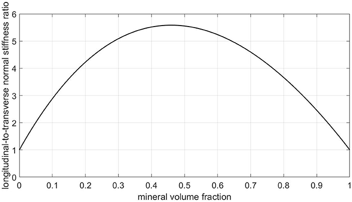
Figure 10. Predictions of a Mori-Tanaka homogenization scheme for a composite model consisting of a collagen matrix with parallel cylindrical mineral inclusions: ratio of longitudinal to transverse normal (homogenized) stiffnesses, as a function of the mineral volume fraction.

Fortunately, all the aforementioned contradictions can be resolved through the new modeling concept provided in the present paper; as this concept was tested, in section 3, against the very data provided by Fratzl et al. [98].

It is also interesting to relate features of the SAXS patterns to underlying ultrastructural characteristics. The results of a corresponding parameter study with the extrafibrillar electron density as the parameter is depicted in Figure 11: As can be referred from Equation (64) with ρ_e,ef = ρ_e,0, the differences in the electron densities, between the gap and extrafibrillar domains on the one hand, and between the overlap and the extrafibrillar domains on the other, are key to the shape of the corresponding SAXS patterns. In more detail, the closer the ratio of the aforementioned differences goes to one, the less the even and odd peaks of the SAXS differ from each other (the green line in Figure 11 refers to the aforementioned ratio being exactly one, while the black and purple lines, respectively, are referring to ratios of 0.79 and 1.27, respectively). Furthermore, the absolute values of the differences in electron density, between the fibrillar and the extrafibrillar spaces, govern the SAXS peak sizes; growing differences being related to diminishing peak sizes (the green line refers to the smallest difference in electron densities, and the red line to the largest one).

FIGURE 11

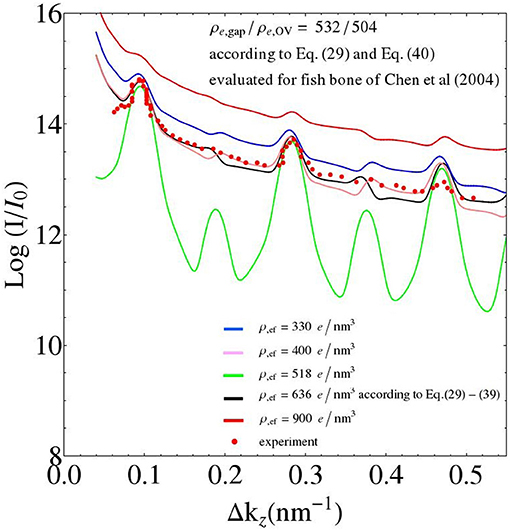
Figure 11. Parameter study: changing the value of the electron density of the extrafibrillar space; while keeping the electron densities of the gap and overlap zones constant (adopting the values from the fish bone simulation of Figure 7).

One may speculate that such information on the characteristics of electron density distribution might serve as additional interesting fingerprints of bone diseases, in addition to those reported by Roschger et al. [112]. However, a more in-depth investigation of this issue would require a considerably larger database of SAXS patterns across different bones under different pathological conditions, as it is available at the present point in time. Anyway, the translation of such differences into corresponding bone strength values seems to be the minor challenge in this context, given recent developments in the multiscale mechanics of bone strength [40, 43].

Conclusively, the microstructural representation of bone ultrastructure essential for the micromechanics of the material, also shows great potential when it comes to predicting SAXS patterns arising from electromagnetic waves hitting bone samples. In this context, the present contribution may be seen as an extension of earlier work of Suhonen et al. [113] for unmineralized tissues, toward the realm of bone. At the same time, it is obvious that the deviations of model predictions from experiments beyond $\Delta k_z>0.35{\mathrm{\text{ nm}}}^{-1}$ may motivate additional investigations toward a more refined ultrastructural representation, and also the prediction of SAXS patterns emerging through bone under mechanical load, based on devices pioneered by Gupta et al. [111, 114] and Karunaratne et al. [115], appears as an interesting topic for the future. At the same time, the current developments may also serve as a basis for a deeper investigation of configurational changes provoked by excessive mechanical loading of soft tissues, such changes having gained recent interest both experimentally [116, 117], and computationally [118].

Author Contributions

CH and PH initiated the project idea. CM, PH, AK, and CH developed the study concept and theory. AK, CM, PH, and TA performed the computations. AK and CH wrote the paper. All authors revised the paper and approved the submitted version.

Funding

Financial support in the framework of project ERC-2010-StG-257023-MICROBONE is gratefully acknowledged. The cooperation between TU Wien and EMSE was facilitated by the bilateral Hubert Curien – Amadeus travel grant FR02/2015 of OEAD – Austrian Agency for International Cooperation in Education and Research on the one hand, and Campus France – French Agency for International Cooperation in Education and Research, on the other. Additional support in the framework of COST action CA 16122 BIONECA is gratefully acknowledged. Moreover, the authors acknowledge the TU Wien Library for financial support through its Open Access Funding Program.

Conflict of Interest Statement

The authors declare that the research was conducted in the absence of any commercial or financial relationships that could be construed as a potential conflict of interest.

Supplementary Material

The Supplementary Material for this article can be found online at: https://www.frontiersin.org/articles/10.3389/fphy.2018.00125/full#supplementary-material

Nomenclature

References

1. Lees S, Bonar LC, Mook HA. A study of dense mineralized tissue by neutron diffraction. Int J Biol Macromol. (1984) 6:321–6. doi: 10.1016/0141-8130(84)90017-5

CrossRef Full Text | Google Scholar

2. Bonar LC, Lees S, Mook H. Neutron diffraction studies of collagen in fully mineralized bone. J Mol Biol. (1985) 181:265–70. doi: 10.1016/0022-2836(85)90090-7

PubMed Abstract | CrossRef Full Text | Google Scholar

3. Lees S. Considerations regarding the structure of the mammalian mineralized osteoid from viewpoint of the generalized packing model. Connect Tissue Res. (1987) 16:281–303. doi: 10.3109/03008208709005616

PubMed Abstract | CrossRef Full Text | Google Scholar

4. Lees S, Prostak K, Ingle VK, Kjoller K. The loci of mineral in turkey leg tendon as seen by atomic force microscope and electron microscopy. Calc Tissue Int. (1994) 55:180–9. doi: 10.1007/BF00425873

PubMed Abstract | CrossRef Full Text | Google Scholar

5. Prostak K, Lees S. Visualization of crystal-matrix structure. In situ demineralization of mineralized turkey leg tendon and bone. Calc Tissue Int. (1996) 59:474–9.

PubMed Abstract | Google Scholar

6. Jantou V, Turmaine M, West GD, Horton MA, McComb DW. Focused ion beam milling and ultramicrotomy of mineralised ivory dentine for analytical transmission electron microscopy. Micron (2009) 40:495–501. doi: 10.1016/j.micron.2008.12.002

PubMed Abstract | CrossRef Full Text | Google Scholar

7. McNally EA, Schwarcz HP, Botton GA, Arsenault AL. A model for the ultrastructure of bone based on electron microscopy of ion-milled sections. PLoS ONE (2012) 7:e29258. doi: 10.1371/journal.pone.0029258

PubMed Abstract | CrossRef Full Text | Google Scholar

8. Schwarcz HP, McNally EA, Botton GA. Dark-field transmission electron microscopy of cortical bone reveals details of extrafibrillar crystals. J Struct Biol. (2014) 188:240–8. doi: 10.1016/j.jsb.2014.10.005

PubMed Abstract | CrossRef Full Text | Google Scholar

9. Sasaki N, Tagami A, Goto T, Taniguchi M, Nakata M, Hikichi K. Atomic force microscopic studies on the structure of bovine femoral cortical bone at the collagen fibril-mineral level. J Mater Sci. (2002) 13:333–7. doi: 10.1023/A:1016199404342

PubMed Abstract | CrossRef Full Text | Google Scholar

10. Hassenkam T, Fantner GE, Cutroni JA, Weaver JC, Morse DE, Hansma PK. High-resolution AFM imaging of intact and fractured trabecular bone. Bone (2004) 35:4–10. doi: 10.1016/j.bone.2004.02.024

PubMed Abstract | CrossRef Full Text | Google Scholar

11. Bozec L, Groot J, Odlyha M, Nicholls B, Nesbitt S, Flanagan A, et al. Atomic force microscopy of collagen structure in bone and dentine revealed by osteoclastic resorption. Ultramicroscopy (2005) 105:79–89. doi: 10.1016/j.ultramic.2005.06.021

PubMed Abstract | CrossRef Full Text | Google Scholar

12. Anderson HC. Molecular biology of matrix vesicles. Clin Orthopaed Relat Res. (1995) 314:266–80.

Google Scholar

13. Anderson HC, Garimella R, Tague SE. The role of matrix vesicles in growth plate development and biomineralization. Front Biosci. (2005) 10:822–37. doi: 10.2741/1576

PubMed Abstract | CrossRef Full Text | Google Scholar

14. Wiesmann HP, Meyer U, Plate U, Höhling HJ. Aspects of collagen mineralization in hard tissue formation. In: Jeon K, editor. International Review of Cytology, Vol. 242. London, UK: Academic Press (2004). p. 121–56.

Google Scholar

15. Katti KS, Avinash AH, Payne S, Katti DR. Vesicular delivery of crystalline calcium minerals to ECM in biomineralized nanoclay composites. Mater Res Exp. (2015) 2:045401. doi: 10.1088/2053-1591/2/4/045401

CrossRef Full Text | Google Scholar

16. Hashin Z, Rosen BW. The elastic moduli of fiber-reinforced materials. J Appl Mech. (1964) 31:223–32. doi: 10.1115/1.3629590

CrossRef Full Text | Google Scholar

17. Halpin JC, Thomas RL. Ribbon reinforcement of composites. J Compos Mater. (1968) 2:488–97.

Google Scholar

18. Sanchez-Palencia E. Non-homogeneous media and vibration theory. Lect Notes Phys. (1980) 127:45–83.

Google Scholar

19. Crolet J, Aoubiza B, Meunier A. Compact bone: numerical simulation of mechanical characteristics. J Biomech. (1993) 26:677–87. doi: 10.1016/0021-9290(93)90031-9

PubMed Abstract | CrossRef Full Text | Google Scholar

20. Aoubiza B, Crolet J, Meunier A. On the mechanical characterization of compact bone structure using the homogenization theory. J Biomech. (1996) 29:1539–47. doi: 10.1016/S0021-9290(96)80005-4

PubMed Abstract | CrossRef Full Text | Google Scholar

21. Ashman R, Cowin S, Van Buskirk W, Rice J. A continuous wave technique for the measurement of the elastic properties of cortical bone. J Biomech. (1984) 17:349–61. doi: 10.1016/0021-9290(84)90029-0

PubMed Abstract | CrossRef Full Text | Google Scholar

22. Katz J. Composite material models for cortical bone. In: Mechanical Properties of Bone, Vol. 45 of AMD. New York, NY: ASME (1981). p. 171–84.

Google Scholar

23. Pidaparti RMV, Chandran A, Takano Y, Turner CH. Bone mineral lies mainly outside collagen fibrils: predictions of a composite model for osternal bone. J Biomech. (1996) 29:909–16. doi: 10.1016/0021-9290(95)00147-6

PubMed Abstract | CrossRef Full Text | Google Scholar

24. Hellmich C, Ulm FJ. Micromechanical model for ultrastructural stiffness of mineralized tissues. J Eng Mech. (2002) 128:898–908. doi: 10.1061/(ASCE)0733-9399(2002)128:8(898)

CrossRef Full Text | Google Scholar

25. Hellmich C, Ulm FJ, Dormieux L. Can the diverse elastic properties of trabecular and cortical bone be attributed to only a few tissue-independent phase properties and their interactions? Arguments from a multiscale approach. Biomech Model Mechanobiol. (2004) 2:219–38. doi: 10.1007/s10237-004-0040-0

PubMed Abstract | CrossRef Full Text | Google Scholar

26. Zaoui A. Continuum micromechanics: survey. J Eng Mech. (2002) 128:808–16. doi: 10.1061/(ASCE)0733-9399(2002)128:8(808)

CrossRef Full Text | Google Scholar

27. Lees S, Page EA. A study of some properties of mineralized turkey leg tendon. Connect Tissue Res. (1992) 28:263–87. doi: 10.3109/03008209209016820

PubMed Abstract | CrossRef Full Text | Google Scholar

28. Lees S, Ahern J, Leonard M. Parameters influencing the sonic velocity in compact calcified tissues of various species. J Acoust Soc Am. (1983) 74:28–33. doi: 10.1121/1.389723

PubMed Abstract | CrossRef Full Text | Google Scholar

29. McCarthy RN, Jeffcott LB, McCartney RN. Ultrasound speed in equine cortical bone: effects of orientation, density, porosity and temperature. J Biomech. (1990) 23:1139–43. doi: 10.1016/0021-9290(90)90006-O

PubMed Abstract | CrossRef Full Text | Google Scholar

30. Rho JY, Hobatho MC, Ashman RB. Relations of mechanical properties to density and CT numbers in human bone. Med Eng Phys. (1995) 17:347. doi: 10.1016/1350-4533(95)97314-F

PubMed Abstract | CrossRef Full Text | Google Scholar

31. Turner C, Cowin S, Rho J, Ashman R, Rice J. The fabric dependence of the orthotropic elastic constants of cancellous bone. J Biomech. (1990) 23:549–61. doi: 10.1016/0021-9290(90)90048-8

PubMed Abstract | CrossRef Full Text | Google Scholar

32. Hamed E, Lee Y, Jasiuk I. Multiscale modeling of elastic properties of cortical bone. Acta Mech. (2010) 213:131–54. doi: 10.1007/s00707-010-0326-5

CrossRef Full Text | Google Scholar

33. Hamed E, Novitskaya E, Li J, Chen PY, Jasiuk I, McKittrick J. Elastic moduli of untreated, demineralized and deproteinized cortical bone: validation of a theoretical model of bone as an interpenetrating composite material. Acta Biomater. (2012) 8:1080–92. doi: 10.1016/j.actbio.2011.11.010

PubMed Abstract | CrossRef Full Text | Google Scholar

34. Sansalone V, Naili S, Bousson V, Bergot C, Peyrin F, Zarka J, et al. Determination of the heterogeneous anisotropic elastic properties of human femoral bone: from nanoscopic to organ scale. J Biomech. (2010) 43:1857–63. doi: 10.1016/j.jbiomech.2010.03.034

PubMed Abstract | CrossRef Full Text | Google Scholar

35. Sansalone V, Naili S, Desceliers C. A stochastic homogenization approach to estimate bone elastic properties. Comptes Rendus Mécanique (2014) 342:326–33. doi: 10.1016/j.crme.2013.12.007

CrossRef Full Text | Google Scholar

36. Hellmich C, Ulm FJ. Average hydroxyapatite concentration is uniform in the extracollagenous ultrastructure of mineralized tissues: evidence at the 1-10 μm scale. Biomech Model Mechanobiol. (2003) 2:21–36. doi: 10.1007/s10237-002-0025-9

CrossRef Full Text | Google Scholar

37. Hellmich C, Barthelemy JF, Dormieux L. Mineral-collagen interactions in elasticity of bone ultrastructure - a continuum micromechanics approach. Eur J Mech. (2004) 23:783–810. doi: 10.1016/j.euromechsol.2004.05.004

CrossRef Full Text | Google Scholar

38. Hellmich C, Ulm F. Microporodynamics of Bones: prediction of the “Frenkel-Biot” Slow Compressional Wave. J Eng Mech. (2005) 131:918–27. doi: 10.1061/(ASCE)0733-9399(2005)131:9(918)

CrossRef Full Text | Google Scholar

39. Fritsch A, Hellmich C. Universal microstructural patterns in cortical and trabecular, extracellular and extravascular bone materials: micromechanics-based prediction of anisotropic elasticity. J Theor Biol. (2007) 244:597–620. doi: 10.1016/j.jtbi.2006.09.013

PubMed Abstract | CrossRef Full Text | Google Scholar

40. Fritsch A, Hellmich C, Dormieux L. Ductile sliding between mineral crystals followed by rupture of collagen crosslinks: experimentally supported micromechanical explanation of bone strength. J Theor Biol. (2009) 260:230–52. doi: 10.1016/j.jtbi.2009.05.021

PubMed Abstract | CrossRef Full Text | Google Scholar

41. Eberhardsteiner L, Hellmich C, Scheiner S. Layered water in crystal interfaces as source for bone viscoelasticity: arguments from a multiscale approach. Comput Methods Biomech Biomed Eng. (2014) 17:48–63. doi: 10.1080/10255842.2012.670227

PubMed Abstract | CrossRef Full Text | Google Scholar

42. Morin C, Hellmich C. A multiscale poromicromechanical approach to wave propagation and attenuation in bone. Ultrasonics (2014) 54:1251. doi: 10.1016/j.ultras.2013.12.005

PubMed Abstract | CrossRef Full Text | Google Scholar

43. Morin C, Vass V, Hellmich C. Micromechanics of elastoplastic porous polycrystals: theory, algorithm, and application to osteonal bone. Int J Plast. (2017) 91:238–67. doi: 10.1016/j.ijplas.2017.01.009

CrossRef Full Text | Google Scholar

44. Laws N. The determination of stress and strain concentrations at an ellipsoidal inclusion in an anisotropic material. J Elast. (1977) 7:91–7. doi: 10.1007/BF00041133

CrossRef Full Text | Google Scholar

45. Laws N. A note on penny-shaped cracks in transversely isotropic materials. Mech Mater. (1985) 4:209–12. doi: 10.1016/0167-6636(85)90017-1

CrossRef Full Text | Google Scholar

46. Fritsch A, Dormieux L, Hellmich C. Porous polycrystals built up by uniformly and axisymmetrically oriented needles: homogenization of elastic properties. Comptes Rendus Mécanique (2006) 334:151–7. doi: 10.1016/j.crme.2006.01.008

CrossRef Full Text | Google Scholar

47. Fritsch A, Dormieux L, Hellmich C, Sanahuja J. Mechanical behavior of hydroxyapatite biomaterials: an experimentally validated micromechanical model for elasticity and strength. J Biomed Mater Res A (2009) 88A:149–61. doi: 10.1002/jbm.a.31727

CrossRef Full Text | Google Scholar

48. Laws N, McLaughlin R. Self-consistent estimates for the viscoelastic creep compliances of composite materials. Proc R Soc A (1978) 359:251–73. doi: 10.1098/rspa.1978.0041

CrossRef Full Text | Google Scholar

49. Dvorak GD. Transformation field analysis of inelastic composite materials. Proc R Soc A (1992) 437:311–27. doi: 10.1098/rspa.1992.0063

CrossRef Full Text | Google Scholar

50. Pichler B, Hellmich C. Estimation of influence tensors for eigenstressed multiphase elastic media with nonaligned inclusion phases of arbitrary ellipsoidal shape. J Eng Mech. (2010) 136:1043–1053. doi: 10.1061/(ASCE)EM.1943-7889.0000138

CrossRef Full Text | Google Scholar

51. Sasaki N, Nakayama Y, Yoshikawa M, Enyo A. Stress relaxation function of bone and bone collagen. J Biomech. (1993) 26:1369–76. doi: 10.1016/0021-9290(93)90088-V

PubMed Abstract | CrossRef Full Text | Google Scholar

52. Iyo T, Maki Y, Sasaki N, Nakata N. Anisotropic viscoelastic properties of cortical bone. J Biomech. (2004) 37:1433–7. doi: 10.1016/j.jbiomech.2003.12.023

PubMed Abstract | CrossRef Full Text | Google Scholar

53. Hosokawa A, Otani T. Ultrasonic wave propagation in bovine cancellous bone. J Acoust Soc Am. (1997) 101:558–62. doi: 10.1121/1.418118

PubMed Abstract | CrossRef Full Text | Google Scholar

54. Hosokawa A, Otani T. Acoustic anisotropy in bovine cancellous bone. J Acoust Soc Am. (1998) 103:2718–22. doi: 10.1121/1.422790

PubMed Abstract | CrossRef Full Text | Google Scholar

55. Reilly DT, Burstein AH. The elastic and ultimate properties of compact bone tissue. J Biomech. (1975) 8:393–405.

PubMed Abstract | Google Scholar

56. Burstein A, Reilly D, Martens M. Aging of bone tissue: mechanical properties. J Bone Joint Surg. (1976) 58:82–6. doi: 10.2106/00004623-197658010-00015

PubMed Abstract | CrossRef Full Text | Google Scholar

57. Riggs CM, Lanyon LE, Boyde A. Functional associations between collagen fibre orientation and locomotor strain direction in cortical bone of the equine radius. Anat Embryol. (1993) 187:231–8. doi: 10.1007/BF00195760

PubMed Abstract | CrossRef Full Text | Google Scholar

58. Chen J, Burger C, Krishnan CV, Chu B, Hsiao BS, Glimcher MJ. In vitro mineralization of collagen in demineralized fish bone. Macromol Chem Phys. (2004) 206:43–51. doi: 10.1002/macp.200400066

CrossRef Full Text | Google Scholar

59. Maxwell J. A dynamical theory of the electromagnetic field. Philos Trans R Soc Lond. (1865) 155:459–512. doi: 10.1098/rstl.1865.0008

CrossRef Full Text | Google Scholar

60. Heaviside O. On the forces, stresses, and fluxes of energy in the electromagnetic field. Philos Trans R Soc Lond. (1892) 183:423–80. doi: 10.1098/rsta.1892.0011

CrossRef Full Text | Google Scholar

61. Born M, Wolf E. Principles of Optics, 7th Edn. Cambridge: Cambridge University Press (1999).

Google Scholar

62. Landau L, Lifshitz E. Course of Theoretical Physics. Vol. 8. Electrodynamics of Continuous Media. Oxford: Pergamon Press (1960).

Google Scholar

63. Raimond J-M. Electromagnétisme et relativité. (2006). Available online at: https://cel.archives-ouvertes.fr/cel-00092954/document

Google Scholar

64. Jenkins F, White H. Fundamentals of Optics. New York, NY: McGraw-Hill (1957).

Google Scholar

65. Vass V, Morin C, Scheiner S, Hellmich C. Review of “Universal” rules governing bone composition, organization, and elasticity across organizational hierarchy. In: Multiscale Mechanobiology of Bone Remodeling and Adaptation, Vol. 578. CISM International Centre for Mechanical Sciences (Vienna: Springer) (2017). p. 175–229.

Google Scholar

66. Morin C, Hellmich C. Mineralization-driven bone tissue evolution follows from fluid-to-solid phase transformations in closed thermodynamic systems. J Theor Biol. (2013) 335:185–97. doi: 10.1016/j.jtbi.2013.06.018

PubMed Abstract | CrossRef Full Text | Google Scholar

67. Lees S. Mineralization of type I collagen. Biophys J. (2003) 85:204–7. doi: 10.1016/S0006-3495(03)74466-X

PubMed Abstract | CrossRef Full Text | Google Scholar

68. Parfitt AM. The physiologic and clinical significance of bone histomorphometric data. In: Recker R, editor. Bone Histomorphometry: Techniques and Interpretation. Boca Raton, FL: CRC Press (1983). p. 143–223.

Google Scholar

69. Skinner HCW, Jahren AH. Biomineralization. In: Holland HD, Turekian KK, editors. Treatise on Geochemistry. Oxford: Pergamon (2007). p. 1–69.

Google Scholar

70. Parry DAD, Craig AS. Growth and development of collagen fibrils in connective tissues. In: Motta P, Ruggeri A (editors). Ultrastructure of the Connective Tissue Matrix. Electron Microscopy in Biology and Medicine (Current Topics in Ultrastructural Research), Vol 3. (Boston, MA: Springer) (1980).

Google Scholar

71. Scott J, Orford C, Hughes E. Proteoglycan-collagen arrangements in developing rat tail tendon: an electron-microscopical and biochemical investigation. Biochem J. (1981) 195:573–81. doi: 10.1042/bj1950573

PubMed Abstract | CrossRef Full Text | Google Scholar

72. Silver F, Kato Y, Ohno M, Wasserman A. Analysis of mammalian connective tissue: relationship between hierarchical structures and mechanical properties. J Long-Term Effect Med Implants (1992) 2:165–98.

PubMed Abstract | Google Scholar

73. Walters B, Stegemann J. Strategies for directing the structure and function of three-dimensional collagen biomaterials across length scales. Acta Biomater. (2014) 10:1488–501. doi: 10.1016/j.actbio.2013.08.038

PubMed Abstract | CrossRef Full Text | Google Scholar

74. Lees S, Mook H. Equatorial diffraction spacing as a function of water content in fully mineralized cow bone determined by neutron diffraction. Calc Tissue Int. (1986) 39:291–2. doi: 10.1007/BF02555221

PubMed Abstract | CrossRef Full Text | Google Scholar

75. Vuong J, Hellmich C. Bone fibrillogenesis and mineralization: quantitative analysis and implications for tissue elasticity. J Theor Biol. (2011) 287:115–30. doi: 10.1016/j.jtbi.2011.07.028

PubMed Abstract | CrossRef Full Text | Google Scholar

76. Urist M, DeLange R, Finerman G. Bone cell differentiation and growth factors. Science (1983) 220:680–6. doi: 10.1126/science.6403986

PubMed Abstract | CrossRef Full Text | Google Scholar

77. Salençon J. Handbook of Continuum Mechanics: General Concepts-Thermoelasticity. Berlin: Springer (2001).

Google Scholar

78. Morin C, Hellmich C, Henits P. Fibrillar structure and elasticity of hydrating collagen: a quantitative multiscale approach. J Theor Biol. (2013) 317:384–93. doi: 10.1016/j.jtbi.2012.09.026

PubMed Abstract | CrossRef Full Text | Google Scholar

79. Lees S, Heeley J. Density of a sample bovine cortical bone matrix and its solid constituent in various media. Calc Tissue Int. (1981) 33:499–504. doi: 10.1007/BF02409480

PubMed Abstract | CrossRef Full Text | Google Scholar

80. Fraser R, MacRae T, Miller A. X-ray diffraction patterns of alfa-fibrous proteins. J Mol Biol. (1965) 14:432–42. doi: 10.1016/S0022-2836(65)80193-0

CrossRef Full Text | Google Scholar

81. Hodge AJ, Petruska JA. Recent studies with the electron microscope on ordered aggregates of the tropocollagen molecule. In: Ramachandran GN, editor. Aspects of Protein Structure - Proceedings of a Symposium held in Madras 14 - 18 January 1963 and organized by the University of Madras. London; New York: Academic Press (1963). p. 289–300.

Google Scholar

82. Brodsky BB, Eikenberry EF. Characterization of fibrous forms of collagen. Methods Enzymol. (1982) 82:127–74.

PubMed Abstract | Google Scholar

83. Piez KA, Trus BL. A new model for packing of type-I collagen molecules in the native fibril. Biosci Rep. (1981) 1:801–10.

PubMed Abstract | Google Scholar

84. Fraser RDB, MacRae TP, Miller A. Molecular packing in type I collagen fibrils. A model with neighbouring collagen molecules aligned in axial register. J Mol Biol. (1987) 193:115–25. doi: 10.1016/0022-2836(87)90631-0

PubMed Abstract | CrossRef Full Text | Google Scholar

85. Wess TJ, Hammersley AP, Wess L, Miller A. Molecular packing of type I collagen in tendon. J Mol Biol. (1998) 275:255–67. doi: 10.1006/jmbi.1997.1449

PubMed Abstract | CrossRef Full Text | Google Scholar

86. Orgel JPRO, Miller A, Irving TC, Fischetti RF, Hammersley AP, Wess TJ. The in situ supermolecular structure of type I collagen. Structure (2001) 9:1061–1069. doi: 10.1016/S0969-2126(01)00669-4

PubMed Abstract | CrossRef Full Text | Google Scholar

87. Lee D, Glimcher M. Three-dimensional spatial relationship between the collagen fibrils and the inorganic calcium phosphate crystals of pickerel (Americanus americanus) and herring (Clupea harengus) bone. J Mol Biol. (1991) 217:487–501. doi: 10.1016/0022-2836(91)90752-R

PubMed Abstract | CrossRef Full Text | Google Scholar

88. Briki F, Busson B, Doucet J. Organization of microfibrils in keratin fibers studied by X-ray scattering. Biochim Biophys Acta (1998) 1429:57–68. doi: 10.1016/S0167-4838(98)00216-7

PubMed Abstract | CrossRef Full Text | Google Scholar

89. Hosemann R, Bagchi S. Direct Analysis of Diffraction by Matter. Amsterdam: North-Holland (1962).

90. Hosemann R, Hindeleh A. Structure of crystalline and paracrystalline condensed matter. J Macromol Sci. (1995) 34:327–56. doi: 10.1080/00222349508219497

CrossRef Full Text | Google Scholar

91. Eads JL, Millane RP. Diffraction by the ideal paracrystal. Acta Crystallogr A (2001) 57:507–17. doi: 10.1107/S0108767301006341

PubMed Abstract | CrossRef Full Text | Google Scholar

92. Rose C, Smith M. The multivariate normal distribution. Math J. (1996) 6:32–7.

Google Scholar

93. Biltz R, Pellegrino E. The chemical anatomy of bone. J Bone Joint Surg. (1969) 51-A:456–66. doi: 10.2106/00004623-196951030-00003

CrossRef Full Text | Google Scholar

94. Parry DAD. The molecular fibrillar structure of collagen and its relationship to the mechanical properties of connective tissue. Biophys Chem. (1988) 29:195–209.

PubMed Abstract | Google Scholar

95. Burger C, Zhou HW, Sics I, Hsiao BS, Chu B, Graham L, et al. Small-angle X-ray scattering of intramuscular fish bone: collagen fibril superstructure determined from equidistant meridional reflections. J Appl Crystallogr. (2008) 41:252–61. doi: 10.1107/S0021889808000277

CrossRef Full Text | Google Scholar

96. Hellmich C, Ulm FJ. Are mineralized tissues open crystal foams reinforced by crosslinked collagen?- Some energy arguments. J Biomech. (2002) 35:1199–212. doi: 10.1016/S0021-9290(02)00080-5

PubMed Abstract | CrossRef Full Text | Google Scholar

97. Schwarcz HP, Abueidda D, Jasiuk I. The ultrastructure of bone and its relevance to mechanical properties. Front Phys. (2017) 5:39. doi: 10.3389/fphy.2017.00039

CrossRef Full Text | Google Scholar

98. Fratzl P, Fratzl-Zelman N, Klaushofer K, Vogl G, Koller K. Nucleation and growth of mineral crystals in bone studied by Small-Angle X-Ray Scattering. Calc Tissue Int. (1991) 48:407–13. doi: 10.1007/BF02556454

PubMed Abstract | CrossRef Full Text | Google Scholar

99. Lu Y, Thiagarajan G, Nicolella DP, Johnson ML. Load/strain distribution between ulna and radius in the mouse forearm compression loading model. Med Eng Phys. (2012) 34:350–6. doi: 10.1016/j.medengphy.2011.07.022

PubMed Abstract | CrossRef Full Text | Google Scholar

100. Zhao L, Shim JW, Dodge TR, Robling AG, Yokota H. Inactivation of Lrp5 in osteocytes reduces Young's modulus and responsiveness to the mechanical loading. Bone (2013) 54:35–43. doi: 10.1016/j.bone.2013.01.033

PubMed Abstract | CrossRef Full Text | Google Scholar

101. Thiagarajan G, Lu Y, Dallas M, Johnson ML. Experimental and finite element analysis of dynamic loading of the mouse forearm. J Orthopaed Res. (2014) 32:1580–8. doi: 10.1002/jor.22720

PubMed Abstract | CrossRef Full Text | Google Scholar

102. Rinnerthaler S, Roschger P, Jakob HF, Nader A, Klaushofer K, Fratzl P. Scanning small angle X-ray scattering analysis of human bone sections. Calc Tissue Int. (1999) 64:422–9. doi: 10.1007/PL00005824

PubMed Abstract | CrossRef Full Text | Google Scholar

103. Wess T, Alberts I, Hiller J, Chamberlain MDAT, Collins M. Microfocus small angle X-ray scattering reveals structural features in archaeological bone samples; detection of changes in bone mineral habit and size. Calc Tissue Int. (2002) 70:103–10. doi: 10.1007/s002230020045

PubMed Abstract | CrossRef Full Text | Google Scholar

104. Grabner B, Landis WJ, Roschger P, Rinnerthaler S, Peterlik H, Klaushofer K, et al. Age- and genotype-dependence of bone material properties in the osteogenesis imperfecta murine model (oim). Bone (2001) 29:453–7. doi: 10.1016/S8756-3282(01)00594-4

PubMed Abstract | CrossRef Full Text | Google Scholar

105. Turunen MJ, Kaspersen JD, Olsson U, Guizar-Sicairos M, Bech M, Schaff F, et al. Bone mineral crystal size and organization vary across mature rat bone cortex. J Struct Biol. (2016) 195:337–44. doi: 10.1016/j.jsb.2016.07.005

PubMed Abstract | CrossRef Full Text | Google Scholar

106. Mori T, Tanaka K. Average stress in matrix and average elastic energy of materials with misfitting inclusions. Acta Metall. (1973) 21:571–4. doi: 10.1016/0001-6160(73)90064-3

CrossRef Full Text | Google Scholar

107. Benveniste Y. A new approach to the application of Mori-Tanaka's theory in composite materials. Mech Mater. (1987) 6:147–57.

Google Scholar

108. Sasaki N, Odajima S. Stress-strain curve and youngs modulus of a collagen molecule as determined by the x-ray diffraction technique. J Biomech. (1996) 29:655–8.

Google Scholar

109. Katz JL, Ukraincik K. On the anisotropic elastic properties of hydroxyapatite. J Biomech. (1971) 4:221–7. doi: 10.1016/0021-9290(71)90007-8

PubMed Abstract | CrossRef Full Text | Google Scholar

110. Bragg WL. The diffraction of short electromagnetic waves by a crystal. Proc Camb Philos Soc Math Phys Sci. (1913) 17:43–57.

Google Scholar

111. Gupta HS, Seto J, Wagermaier W, Zaslansky P, Boesecke P, Fratzl P. Cooperative deformation of mineral and collagen in bone at the nanoscale. Proc Natl Acad Sci USA. (2006) 103:17741–6. doi: 10.1073/pnas.0604237103

PubMed Abstract | CrossRef Full Text | Google Scholar

112. Roschger P, Paschalis EP, Fratzl P, Klaushofer K. Bone mineralization density distribution in health and disease. Bone (2008) 42:456–66. doi: 10.1016/j.bone.2007.10.021

PubMed Abstract | CrossRef Full Text | Google Scholar

113. Suhonen H, Fernandez M, Serimaa R, Suortti P. Simulation of small-angle x-ray scattering from collagen fibrils and comparison with experimental patterns. Phys Med Biol. (2005) 50:5401–16. doi: 10.1088/0031-9155/50/22/012

PubMed Abstract | CrossRef Full Text | Google Scholar

114. Gupta HS, Wagermaier W, Zickler GA, Raz-Ben Aroush D, Funari SS, Roschger P, et al. Nanoscale deformation mechanisms in bone. Nano Lett. (2005) 5:2108–111. doi: 10.1021/nl051584b

PubMed Abstract | CrossRef Full Text | Google Scholar

115. Karunaratne A, Esapa CR, Hiller J, Boyde A, Head R, Bassett JHD, et al. Significant deterioration in nanomechanical quality occurs through incomplete extrafibrillar mineralization in rachitic bone: evidence from in-situ synchrotron X-ray scattering and backscattered electron imaging. J Bone Mine Res. (2012) 27:876–90. doi: 10.1002/jbmr.1495

PubMed Abstract | CrossRef Full Text | Google Scholar

116. Krasny W, Magoariec H, Morin C, Avril S. Kinematics of collagen fibers in carotid arteries under tension-inflation loading. J Mech Behav Biomed Mater. (2017) 77:718–26. doi: 10.1016/j.jmbbm.2017.08.014

PubMed Abstract | CrossRef Full Text | Google Scholar

117. Krasny W, Morin C, Magoariec H, Avril S. A comprehensive study of layer-specific morphological changes in the microstructure of carotid arteries under uniaxial load. Acta Biomater. (2017) 57:342–51. doi: 10.1016/j.actbio.2017.04.033

PubMed Abstract | CrossRef Full Text | Google Scholar

118. Morin C, Avril S, Hellmich C. Non-affine fiber kinematics in arterial mechanics: a continuum micromechanical investigation. J Appl Math Mech. (2018). doi: 10.1002/zamm.201700360. [Epub ahead of print].

CrossRef Full Text | Google Scholar