Modeling Active Cell Movement With the Potts Model

In the last decade, the cellular Potts model has been extensively used to model interacting cell systems at the tissue-level. However, in early applications of this model, cell movement was taken as a consequence of membrane fluctuations due to cell-cell interactions, or as a response to an external chemotactic gradient. Recent findings have shown that eukaryotic cells can exhibit persistent displacements across scales larger than cell size, even in the absence of external signals. Persistent cell motion has been incorporated to the cellular Potts model by many authors in the context of collective motion, chemotaxis and morphogenesis. In this paper, we use the cellular Potts model in combination with a random field applied over each cell. This field promotes a uniform cell motion in a given direction during a certain time interval, after which the movement direction changes. The dynamics of the direction is coupled to a first order autoregressive process. We investigated statistical properties, such as the mean-squared displacement and spatio-temporal correlations, associated to these self-propelled in silico cells in different conditions. The proposed model emulates many properties observed in different experimental setups. By studying low and high density cultures, we find that cell-cell interactions decrease the effective persistent time.

1. Introduction

Biological development is a clear example of a complex system and is the result of several morphogenetic processes such as: cell adhesion, cell division, migration, among others [1]. Important insights about the principles involved in the biological development can be extracted from mathematical models used in many works over the last decade [2]. However, there is still no standard model to describe interacting cells in all scales. A suitable approach depends on the spatial and temporal scale associated to the question under study [3, 4]. Continuous models to study combinations of chemical reaction kinetics and cell mobilities through diffusional processes have been useful at tissue-level scales [5, 6]. Also, simplified continuous models of self-propelled particles have been useful to uncover a new kind of phase transition in collective motions [7–12], (see [13] for a review of motility-induced phase separation).

However, these models could not be adequate to analyze biological processes involving adhesion and/or changes in cell shapes. On the other hand, cell-based models, such as the lattice-gas cellular automaton [14, 15] or cellular Potts models (CPM) [16, 17] offer a better choice to analyze interacting cell systems at the tissue-level. These discrete models usually do not incorporate physical-chemical processes in detail, since it would imply covering a broad range of scales, and are not amenable to mathematical analysis. However, particularly CPM has been shown to be suitable for studying very complex phenomena, via computer simulations. In this sense it has been applied successfully in the study of cell sorting in cellular aggregates [16, 18], morphological development of the Dictyostelium discoideum slug [19–21], and tumor growth and angiogenesis [22, 23]. Recently, a continuum limit of the CPM was proposed to study the role of membrane elasticity on the migration potential of cancer cells [24].

CPM was introduced by Glazier and Granier in '90 [16, 18], as an extended large-Q Potts model. CPM considers individual cells, which can suffer small deformations and volume changes according to a free energy minimization principle which drives its dynamics. As a consequence of the small changes resulting from cell interactions with elements of their immediate surrounding, the cells perform small displacements (≪ cell size [25]). Statistical properties of this “passive" movement of in silico cells in aggregates have also been studied [26, 27]. With this model, cells perform a random walk; i.e., the position and velocity power spectra correspond to Brownian motion and the velocities are time-uncorrelated. Although some correlations have been detected both in Hydra cell aggregates [28] and in Madin-Darby canine kidney cells [29, 30], this finding is in agreement with experiments performed with pigmented retinal cells [26].

Cell motion is usually influenced by processes that involve several components of the cellular migration machinery, resulting in cell polarization. When the direction of polarization is maintained in time the cell can perform a persistent movement. This active movement has been observed in collective migration both in response to external chemotactic gradients [31], as well as in the absence of external signals [29, 30, 32–34]. Persistent polarization, intermittency and changes in the movement direction are consequently reflected in strong spatial and temporal correlations [29, 30]. In order to direct cell motion in the CPM framework, researchers have added terms to the differential of the Hamiltonian that drive a directional bias of cell movement. Thus, a term has been introduced to model the chemotactic response of Dictyostelium cells in response to cAMP signaling during the slug morphogenesis [35]. Similar bias terms have been proposed for making cell motility dependent on a propensity vector, thus modeling persistent, active cell motility in absence of external fields [33, 36].

In the same direction, it has been used more recently in the context of collective cell migration or active matter [37, 38]. These simplified models consider persistent cell motion externally embedded in the CPM. In contrast, some efforts have been devoted to build models that include an actin-based mechanism resulting in cell protrusions and, consequently, in active cell movement [39], or even more detailed models that integrate the biochemical reactions and cytoskeleton dynamics to cell motion [40]. These multiscale models can be used to understand how molecular-based mechanisms give rise to the epiphenomenon of persistent cell motion in the absence of external signals.

In this paper, we study the effects of low and high density cultures in persistent cell movement when external signals are absent. For this purpose we use the CPM, which considers cell adhesion and deformation, to better describe cell-cell interactions. Alternatively, one can use a particle-based model with volume exclusion, but in our opinion this is not the best way to consider interaction between cells. Therefore, we propose a modification in the dynamics of the directional propensity vector introduced in previous works that consider active cell movement in the absence of external cues [33, 36]. In this sense, we link the polarization direction of the cell to an autoregressive process that changes the migration direction after some characteristic time τ, and study the dynamics of the resulting cell movements. We perform computer simulations for different parameter values and find that the dynamics of these in silico-cell movements resembles the behavior observed experimentally in the absence of external signals [34, 41]. We believe that the present modeling approach can fill the gap between interesting characteristics of the cell motility (correlations, velocity distributions) and key ingredients, such as persistence time and cell density.

2. Methods

2.1. The Model

The CPM has been introduced as an extension of the Potts model, which is a generalization of the Ising model. The CPM has been used in literature by many authors to study a wide range of phenomena, ranging from critical behaviors of bubbles to cellular arrangements [42]. The model basically consists of a system of interacting spins σ on a lattice, where the set of all (adjacent) sites with the same spin defines a cell. Different terms of energy can be considered according to the purpose of each case study. In the basic model, the energy E₀ is associated with the cell-cell interaction, cell volumes [18], and cell perimeters [27]. Fluctuations of the membrane allow the cells to explore their neighborhood. Thus, if the total number of cells is Q, all sites i where σ_i = M, with 1 ≤ M ≤ Q, belong to the cell labeled as M. The energy of any configuration of cells is given by

$\begin{array}{l}{E}_0=-{\displaystyle \underset{i,j}{{\sum }^{\prime }}}{J}_{{\sigma }_i{\sigma }_j}(1-{\delta }_{{\sigma }_i{\sigma }_j})+{\displaystyle \sum _{M=1}^Q}\kappa {(A_M-A_0)}^2+\\ +{\displaystyle \sum _{M=1}^Q}\Gamma {(L_M-L_0)}^2,& (1)\end{array}$

where the primed sum runs over neighboring site pairs and δ_σiσj is the Kronecker delta, and equals one if σ_i = σ_j and zero otherwise. Thus, the first sum is over all neighboring site pairs of adjacent cells, and represents the boundary energy of the interacting cells. The second and third sums represent the energies of area and perimeter elasticities of the cells, respectively, and are related with the constants κ and Γ. In this way, a target area A₀ and a target perimeter L₀ are introduced and the sums are over all cells on the lattice, being A_M and L_M the area and perimeter of the cell M. The second and third terms on Equation (1) are required to generate domains of spins resembling cells, that will not break nor disappear, in a sustained manner over time [27]. As we will see later, the presence of a medium, which interacts with the cells, can also be considered by assigning zero value to the spin variable σ_i = 0. Obviously, the medium has neither target area nor target perimeter.

The system evolves using standard Metropolis algorithm, with the following variant: a lattice site i is randomly chosen and if it belongs to the boundary of the cell M, then the site assumes the spin value of its neighboring cell M′ with probability proportional to the Boltzmann factor $e^{(-\Delta E_0/k_{B}T)}$, where ΔE₀ is the change of energy involved in the proposed update and k_BT simulates the energy associated to membrane fluctuations driven by the cytoskeleton [18]. At each Monte Carlo step, the total number of sites is randomly chosen and the probability of the configuration update is evaluated in each case. Thus, according to Equation (1), changes in cell shape and cell displacement are a result of membrane fluctuations alone.

The energy above has been broadly used in CPM to drive the cell movement [26, 42–44]. However, the terms in Equation (1) are insufficient to describe active cell motility, characterized by a persistent direction of cell movement. In order to simulate the active cell movement we consider an additional term in the energy, promoting a bias in the cell extensions toward a given direction, as originally proposed in Savill and Hogeweg [35]. This term has been broadly used in modeling active cell motion both in the presence and absence of external cues [21, 33, 36, 37, 45], acting as a source of energy that drives motility of a given cell M preferentially along the direction of a driving force ${\vec{F}}^M$. Thus, the overall energy variation at each Monte Carlo step can be written as:

$\begin{array}{ll}\Delta E=\Delta E_0+{\displaystyle \sum _{M=1}^Q}{\vec{F}}^M·\Delta {\vec{r}}_M,& (2)\end{array}$

where ΔE₀ is the change of energy due to Equation (1) and $\Delta {\vec{r}}_M$ represents the displacement of the center of cell M.

The driving force is characterized by a strength $F=|{\vec{F}}^M|$ and a direction denoted by Θ_M. Here, while the strength is equal for all cells and constant over time, the driving force direction is different for each cell and evolves independently of the others. In fact, Θ_M is actualized according to the following first-order autoregressive process:

$\begin{array}{ll}{\Theta }_M\left(t^{*}\right)=\varphi {\Theta }_M\left(t^{*}-1\right)+\Delta \Theta ϵ\left(t^{*}\right),& (3)\end{array}$

where t* refers to the time of actualization of Θ_M, which is different from the Monte Carlo time step used to update the configuration of the cells. ϕ and ΔΘ are constant parameters, that can take values between (0, 1) and (0, π), respectively. ϵ(t) is a white noise with zero mean and unit variance (${\sigma }_{ϵ}^2=1$). The stochastic difference Equation (3) can be reinterpreted in terms of the Ornstein-Uhlenbeck process with media zero, dx(t) = −λx(t)dt−σdW(t), where dW(t) denotes the Wiener process. In fact, setting the friction coefficient λ = 1−ϕ and σ = ΔΘ, Equation (3) becomes the discrete-time counterpart of the Ornstein-Uhlenbeck process. Over time, the mean value and the variance of Θ are 〈Θ〉 = 0 and ${\sigma }_{\Theta }^2={\Delta \Theta }^2{\sigma }_{ϵ}^2/(1-{\varphi }^2)$, for ϕ < 1, respectively. On the other hand, the temporal autocorrelation of the angle Θ_M, defined by the quotient between the autocovariance and the variance σ_Θ, is given by

$\begin{array}{ll}{R}_{\Theta }=\frac{\langle \Theta (t^{*})\Theta (t^{*}+n)\rangle }{{\sigma }_{\Theta }^2}~e^{nln\varphi }\text{ with }n=1,2,\dots .& (4)\end{array}$

Thus, the expected overall time decay for a cell movement in a given direction is −τ/ln ϕ. When ϕ closes to 0, the time decay tends to zero and the angle dynamics looks like white noise. But when ϕ approaches 1, ${\sigma }_{\Theta }^2\to \infty$ and the temporal autocorrelation is large. Equation (3) expresses a putative dynamics for the driving force direction. Different update rules have been considered in previous works [33, 36, 37]. In fact we also explore an alternative one, that includes a positive feedback loop, in the Results section.

The movements of the cells do not necessarily have the same direction of the driving force, due both to the stochastic fluctuations and to cell-cell interactions. For example, if the driving force is applied on two adjacent cells in opposite directions and one of them attempts to move in the direction of the other, there is no contribution to the energy variation. In order to avoid confusion, we refer to the angle of the driving force and of displacement of the cell M as Θ_M and α_M, respectively.

2.2. Simulation Details

To compute the energy contribution associated with cell-cell and cell-medium interactions we consider a neighbor range greater than one lattice site. Thus, the primed sum in Equation (1) considers 1st, 2nd, 3rd, and 5th neighbors, which contribute to the energy J_σiσj with weights proportional to the inverse of their distances d_i,j. In short, if σ_i ≠ σ_j ≠ 0, the surface energy J_σiσj = J_cell−cell/d_i,j, where J_cell−cell is the cell-cell adhesion constant. On the other hand, if one of the neighboring sites, i or j, belongs to the medium, the surface energy is given by J_σiσj = J_{cell−medium}/d_i,j, where J_{cell−medium} is cell-medium adhesion constant. Therefore, the first term of Equation (1) contributes to the energy if the sites i and j belong to different cells or one of them belongs to a cell and the other to the medium, representing the cell-cell or cell-medium adhesion, respectively. As cells tend to stick together, we chose J_cell−cell > J_{cell−medium} in our simulations, as we will see next.

The initial configuration is generated by partitioning the lattice into equal-sized square domains, corresponding to the cells, each cell containing 16 × 16 lattice sites. The squares alternate offsets in every other row, so the pattern resembles a brick wall arranged in common bond. This situation corresponds to a dense aggregate of cells which have been adopted in most previous studies. As the diameter of the cell is about 16 pixels, the parameter L₀ and A₀ have been set to π × 16 and π × 64, respectively. For comparison purposes, taking into account that most eukaryotic animal cells have a diameter between 10 and 30 μm, we can establish the equivalence μm = pixel.

In order to understand the role of cell-cell interactions on the statistical characterization of locomotion activity, we also study cellular movement at low and high density cell cultures. To this end, we assign the same spin value to a number of randomly chosen cells, σ_i = 0 associated with the medium. Thus, the zero spin domain represents the medium, whereas the group of spins σ_i = M with 1 ≤ M ≤ Q values, belong to the cell labeled as M. The density ρ is defined as the quotient between the area occupied by cells with σ_i ≠ 0 and the total area, thus ρ = 1 implies a lattice fully populated with cells.

Simulations start with a given cell density ρ, allowing for a “thermalization” time interval on the dynamics to obtain adequate cellular shapes, during which no motility forces are applied on cells. In this thermalization interval, of the order of 100 MCS, the configuration is updated through calculating the Boltzmann factor $e^{-\Delta E_0/k_{B}T}$ according to Equation (1). Once the system thermalizes, we establish the starting time t = 0 (see Figure 1). At this point the dynamics starts, with the presence of the motility force on the cells with constant strength and angle given by Equation (3). The initial angle of each cell, Θ_M(0), is chosen randomly. At each Monte Carlo step the driving force direction for each cell changes with probability 1/τ according to Equation (3), where ${\Theta }_M(t^{*}-1)$ indicates the direction previous to the actualization. Thus, the change in the driving force direction Θ_M occurs at a mean time τ.

FIGURE 1

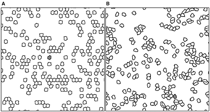
Figure 1. Typical snapshots of a simulation carried out on a lattice of 512 × 512 sites at two different times: (A) initial time (t = 0) in which the dynamic starts with the presence of driving forces acting on each cell, (B) after t = 2, 000 MCS the cells have moved on the medium. For example, gray colored cell has displaced across scales much larger than the cell size. The parameter values used for this simulation were ρ = 0.2, τ = 10 MCS, and ϕ = 0.95.

For all simulations in this paper, we used periodic boundary conditions and a square lattice of size 512 × 512 sites. We have also fixed the parameter values J_cell−cell = 0.1, J_{cell−medium} = 0.01, Γ = 0.2, κ = 1, ΔΘ = π/3, F = 10, and T = 2; while we vary the values of parameters ρ, τ and ϕ in order to study the dynamics of the resulting cell movement. Figure 1 illustrates two instances of the simulation at low density culture (ρ = 0.2), with a driving force $\vec{F}$ of constant module and whose direction is governed by Equation (3). Additionally, the dynamics of the resulting simulation for low and high density cultures can be seen in the Supplementary Movies 1, 2, respectively.

Our selection for ΔΘ avoids a preferential rotation of cells, since the stochastic term in Equation (3) blurs the angle of the previous time. Then, cells perform random walks in the long time scale as we will show in subsection III-C. For small values of ΔΘ cells can display a preferential rotation, which has been observed for cells confined in circular micropatterns [38, 46]. However, the study of geometrical confinement into well-defined circles is outside the scope of this work.

3. Results

Figure 2 shows four different simulated cell trajectories and their associated angles on a 2D substrate using our model with the same parameter values as those used in Figure 1 A combination of persistent and random cell displacements can be seen in Figure 2A. These trajectories resemble those traced by Dictyostelium cells [34], which travel much longer distances than the typical cell size. It is important to note that a constant driving force, when applied to an isolated cell, originates a movement of constant velocity [36]. In this way, the persistent movement in our model is due to the driving force, that has a constant strength and is applied with constant direction during a mean time τ, as discussed before.

FIGURE 2

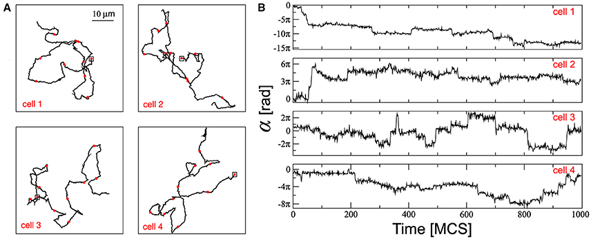
Figure 2. (A) The trajectories are marked off with red circles each 100 MCS and the squares correspond to the positions of each cell at t = 0 MCS. (B) Temporal course of the cell displacement angles α associated with the trajectories depicted on the left panels. Parameters used: ρ = 0.2, τ = 10 MCS, and ϕ = 0.95.

The panels of Figure 2B depict the cumulative cell displacement angle and were obtained by tracking the cell displacement angles with reference to a fixed system. In general, over a short time scale, cells move in a certain direction around which the instantaneous angle direction fluctuates. These fluctuations are due to the cell membrane movement driven by the cytoskeleton and also by cell interactions. At large time scales (>τ) random changes in the cell direction become more apparent and they are promoted by the driving force whose angle actualization is given by Equation (3). Over time, the cumulative cell displacement angle, in addition to offering the instantaneous direction of the cell at a given time, also tracks the entire history of the cell's directional changes. Therefore, periods of persistent cell displacement correspond to constant average angles, while large turns in the cell trajectories are related to large increases or decreases in the average angles. In this way, cell 4 maintains a relatively persistent movement between 30 and 200 MCS (Figure 2A) which is accompanied by a cell displacement angle that fluctuates around the constant value α~−0.8πrad (Figure 2B); and cell 2 presents marked increases and decreases in α around the first 100 MCS (Figure 2B) that correspond to different turns in its trajectory (Figure 2A).

3.1. Cell Displacement

We studied several statistical properties associated to the cell displacement which can be compared with the ones derived from experimental measures. In this sense, we define the cell displacement of a cell M, $\Delta {\vec{r}}_M(t)$ in a time interval Δt, as $({\vec{r}}_M(t+\Delta t)-{\vec{r}}_M(t))$. Associated with this cell displacement, there is a displacement angle α_M(t) and a mean velocity ${\vec{v}}_M(t)=\Delta {\vec{r}}_M(t)/\Delta t$ during this interval.

First of all we consider the cell displacement angle α by using Δt = 1. As shown in the histogram of Figure 3A, cells can move in any direction with similar probabilities, putting in evidence that there is not a preferential direction. This histogram was computed over all cells during a simulation with the same parameter values as those used in 1. Figure 3B depicts the temporal autocorrelation function of α, defined as C_α(t) = Z_α(t)/Z_α(0) where Z_α(t) = 〈α_M(t₀ + t)α_M(t₀)〉, and the averaging was performed over all cells. Besides, the dynamics of α has a characteristic time, which depends on the parameters τ and ϕ, as suggested by expression (4) for Θ. The characteristic time computed in the exponential decay region (inset of Figure 3B) is 194 MCS, in agreement with the theoretical prediction associated to the driving force angle, −τ/ln ϕ = 195 MCS.

FIGURE 3

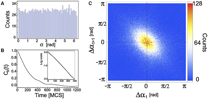
Figure 3. (A) Frequency distribution of cell displacement angle α for all cells during 4,000 MCS. (B) The autocorrelation of α, C_α, as a function of time. Inset: log scale of C_α showing the region of exponential decay (short times). (C) 2D-histogram of the turn angle (Δα_t versus Δα_{t + 1}), showing that two consecutive turn angles are anti-correlated. Parameters used: ρ = 0.2, τ = 10 MCS, and ϕ = 0.95.

Figure 3C depicts a 2D-histogram of the recurrent plot of the turn angles Δθ(t) vs. Δθ(t + 1), where Δθ(t) = θ(t)−θ(t−1). This plot shows that two consecutive turn angles are anti-correlated. This feature of cell motility has also been observed in experiments with Dictyostelium cells [34].

As observed by Cox [34], some statistical properties associated with cell movements depend on the time interval Δt considered. We studied the distribution of the cell velocity components v_x and v_y for different time intervals Δt = 1, 3, 10, and 60 MCS. Figure 4 illustrates the distribution of cell velocities for ϕ = 0.95, τ = 10 and two different densities: ρ = 0.2 (Figure 4A) and ρ = 0.9 (Figure 4B). These distributions were obtained by tracking 51 cells (chosen at random). For Δt = 1, the velocity distributions for both densities are quite similar, resembling Gaussian distributions, but with small gaps in the centers of the plots. However, as Δt increases, the difference between the distributions of the cell velocity components obtained at low and high densities becomes more apparent. When Δt approaches to τ, the gap in the center increases for ρ = 0.2, but not for ρ = 0.9, where it is quite smaller and only apparent for Δt = 3. In fact, the difference between low and high densities is more evident when Δt = τ, indicating that this is an adequate time interval size to characterize the underlying dynamics. Similar results were obtained from simulations by using τ = 50 (Supplementary Figure 1), where the main difference between high and low densities is also found for Δt = τ.

FIGURE 4

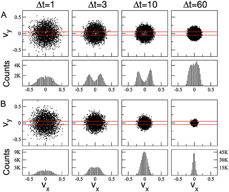
Figure 4. Cell velocities v_x vs v_y calculated for different values of the time interval Δt (upper panels). Histogram of the cell velocity component v_x computed over the v_y window indicated by red bars (lower panels). Two different values of densities were used: ρ = 0.2 (A) and ρ = 0.9 (B). All other parameters are equal to Figure 2.

It is important to note that the gap in the velocity distribution was not observed in simulations performed when the persistence time is absent (i.e., τ = 1, Supplementary Figure 2). Thus, the presence of a gap in the center of the velocity distribution is associated with effective persistent cell movement, in agreement with Maiuri et al. (Figure 4D of [47]). On the other hand, in high density simulations the crater-like effect is less evident (Figure 4B and Supplementary Figure 1). Note that for ρ = 0.9 and Δt = τ the velocity distribution resembles a Gaussian one, indicating that cell-cell interactions, massively present in these cases, contribute to decrease the effective persistent movement of the cells. Large enough values of Δt (>τ) blur the instantaneous direction of cell, and distributions are characterized by a bell shape independently of the densities. Similar results were obtained for ϕ = 0.99 (Supplementary Figure 3), where the behavior of the distributions tails for ρ = 0.9 are more Gaussian than for ϕ = 0.95.

The movement of Dictyostelium cells in the absence of external signals presents a sequence of velocity distributions by varying Δt [34] similar to that obtained from our model, for ρ = 0.2.

3.2. Velocity Correlation

Many studies on cell motility have considered both temporal and spatial correlation functions of the cell velocity for statistical characterization of locomotion activity [25, 28–30, 34]. The temporal autocorrelation function is defined as C(t) = Z(t)/Z(0) where $Z(t)=\langle {\vec{v}}_M(t_0+t)·{\vec{v}}_M(t_0)\rangle$ [25]. The cell velocities ${\vec{v}}_M$ were computed using Δt = 1 MCS, and 〈…〉 indicates the average over all cells and over t₀.

Figure 5A depicts the behavior of C(t) at low density (ρ = 0.2), for three values of the parameter τ = 10, 50, and 100, and two values of ϕ = 0.95 and 0.99. As expected, the correlation decay increases with τ. For ϕ = 0.99 (dashed lines) C(t) exhibits a single exponential decay, which is consistent with an Ornstein-Uhlenbeck process. However, for ϕ = 0.95 (solid lines) C(t) exhibits a more complex behavior: a double exponential decay with a slower decrease at long time scales, independent of the τ value. Moreover, as expected, the autocorrelation function associated to the driving force with ϕ = 0.95 is greater than that obtained from the more random driving force, ϕ = 0.99. We also notice that the behavior of C(t), obtained with the same ϕ but different τ values, coalesces when it is scaled with the parameter τ (Figure 5C).

FIGURE 5

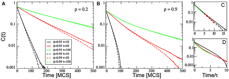
Figure 5. Semi-log plot of the temporal autocorrelation function C(t) averaged over all cells in the simulation. The plots correspond to three different values of τ, two values of ϕ (0.95 solid lines and 0.99 dashed lines) and for two different densities: ρ = 0.2 (A) and ρ = 0.9 (B). (C,D) Shows the collapse of the curves by rescaling the horizontal axes by τ, for the simulations at low and high density, respectively. All other parameters values are the same as in Figure 2.

However, the effects of the cell-cell contact on the autocorrelation function are much more complex. Similar simulations to those used in Figure 5A but at a higher density, ρ = 0.9, show that C(t) does not exhibit a single exponential decay in none of the cases studied (Figure 5B). On the other hand, the effect of the density on the decay of the autocorrelation function depends on the value of the persistence time τ. In this sense, when comparing short and long-time behavior, we can observe that the decay rate increases at long time scales for τ = 10, while it decreases for τ = 100. Consequently, the behavior of C(t) for different τ values does not coalesce when scaled with τ (Figure 5D). We found that the temporal autocorrelation obtained at high density cultures is smaller than at low density cultures. This fact can be understood in terms of the decrease of the effective persistence time of cell movements due to a crowded neighborhood, as seen also in Figure 4.

Spatial correlations of the cell velocities have also been used to characterize the dynamics [25, 28, 29]. The spatial correlation is defined as $C(r)=\langle {\vec{v}}_M·{\vec{v}}_{M^{\prime }}/(|{\vec{v}}_M||{\vec{v}}_{M^{\prime }}|)\rangle$, with $r=|{\vec{r}}_M-{\vec{r}}_{M^{\prime }}|$ the distance between mass center of cells M and M′ [25]. Figure 6 shows C(r) for two different cell densities on the substrate, ρ = 0.2 and 0.9 (solid and dashed lines, respectively), and three different values of τ. These curves display a peak around 14–16 pixels, close to the diameter of a non-interacting cell. Since the in silico cells have an elastic membrane, they can be deformed to reach intercellular distances smaller than the cell diameter. This can occur when the cells travel in opposite directions or in order to increase the contact area. In Figure 6 one can observe that at very short distances (r < 8 pixels) cells are anti-correlated. The negative values for the spatial correlation correspond to cell-pairs in collision, i.e., cells traveling in opposite directions. These cell-pairs are also present, in less extent, in the range 8 ≤ r ≲ 14 pixels, contributing to lower the correlation. Thus, in this range, one can observe that C(r) obtained for simulations at low density are higher than the ones obtained at high densities, in particular for τ = 10. However, for longer distances (r ≳ 16 = cell diameter) this relationship is inverted, i.e., cells in high density configurations are more correlated. Besides, C(r) in high density simulations approaches zero very slowly, as r increases. These results are independent of the τ-value, indicating that the cell-cell contact induces long-range spatial-correlation of cell velocity. Interestingly, highly correlated motions have been found in crowded tissues [6] and in cells in different aggregate types [28]. Experimentally, high spatial correlations have been found in cell aggregates moving together collectively [29].

FIGURE 6

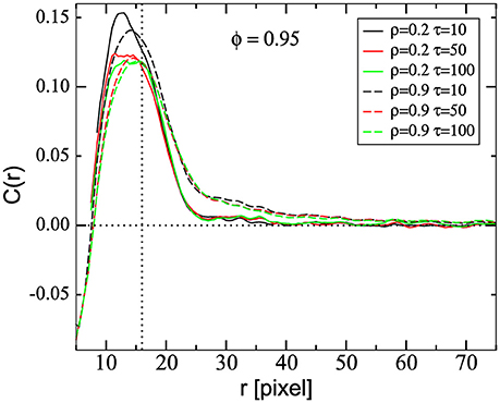
Figure 6. Average spatial correlation function of the velocities, C(r), as a function of the distance r between cell pairs, for two different densities, ρ = 0.2 and 0.9 (continuous and dashed lines, respectively) and different values of τ, as indicated, and ϕ = 0.95. The vertical dashed line represents the average cell diameter equal to 16 μm as discussed in section 2.2. Data was obtained by averaging between 0 and 4,000 MCS and over 50 and 10 samples, for ρ = 0.2 and 0.9, respectively.

At intermediate distances C(r) decays exponentially allowing to define a correlation length. We found that, the correlation lengths obtained for ρ = 0.9 are larger than those obtained using ρ = 0.2, independently of the τ-value. Also, for ρ = 0.9, simulations with τ = 10 present a slightly smaller correlation length than simulations with τ = 50 and 100 (9.1, 10.2, and 11.0, respectively). This means that correlation length increases with cell velocity, as cell velocity also increases with τ. This fact is in agreement with previous findings reporting the increase of correlation length with cell velocities [48]. On the other hand, for ρ = 0.2, all simulations present similar values for the correlation length (5.2, 5.4, and 5.4 for τ = 10, 50, and 100, respectively).

Note that, according to Equation (3) the angle of the driving force Θ_M depends on its previous value but does not depend on the direction of the cell movement α_M. Other authors have considered the presence of a positive feedback loop in cell polarization dynamics, in which cell produces its own chemotactic signal [33, 36, 37]. In order to take into account this feedback loop, an alternative way to update the angle Θ_M is:

$\begin{array}{ll}{\Theta }_M(t^{*})=\varphi \overline{{\alpha }_M(t^{*})}+\Delta \Theta ϵ(t^{*}),& (5)\end{array}$

where $\overline{{\alpha }_M(t^{*})}$ is the mean displacement angle over the last τ MCS, and the other parameters are the same as in Equation (3). Thus, according to Equation (5) the angle of the driving force depends on the earlier cell displacements with a weight given by the parameter ϕ.

We observe that, for any cell density, both the temporal and spatial correlations of the cell velocities are higher when using Equation (5) instead of Equation (3) (see Supplementary Figures 4, 5). In particular, the increment in the correlations is more evident for ρ = 0.9, indicating that the differences between the angle update rules are more apparent in crowded cell cultures. C(t) obtained when considering Equation (5) for ρ = 0.2 is almost independent of the parameter ϕ, whereas for ρ = 0.9 short and long-time behavior of C(t) depends on τ and ϕ in a non trivial manner (see Supplementary Figure 4). Again, the correlation length obtained with Equation (5) increases with τ, reaching 1.6-fold of the cell size when τ = 100 (see Supplementary Figure 5). However, this value is smaller than the correlation length of 2–3 cell size, reported in Garcia et al. [48]. Interestingly, when a feedback from previous displacements is taken into account through Equation (5), C(r) is less negative at very short distances, suggesting that adjacent cells can be avoided in a more realistic way.

3.3. Mean-Squared Displacement

The mean-squared displacement (MSD) is a useful measure to find cell persistence of migration in two and three dimension microenvironments [49–52]. This is calculated as $\mathrm{\text{MSD}}(t)=\langle {({\vec{r}}_M(t)-{\vec{r}}_M(0))}^2\rangle$, where 〈…〉 indicates the average taken over all the cells on the substrate. Figure 7 shows MSD scaled with time as a function of time at ρ = 0.2 (solid lines) and at ρ = 0.9 (dashed lines) and three different values of τ. The MSD obtained for high density is lower than that obtained for low density, as expected. In all cases, MSD behaves as ~t² for short enough time scales (ballistic), and MSD behaves as ~t for long time scales (random walk), as expected for cell movements in the absence of symmetry-breaking gradients [34, 41]. Scaling MSD with τ² and the time with τ, we can observe that the scaled behavior is independent of ϕ and τ for ρ = 0.2. However, for high density, there is a small deviation and scaled behavior depends on the τ-value, showing the complex behavior generated by the interaction between cells.

FIGURE 7

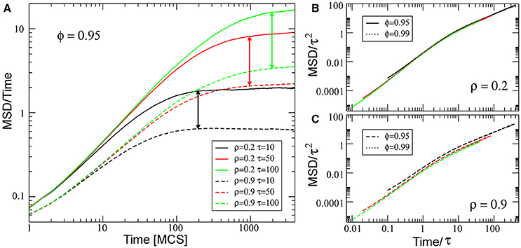
Figure 7. (A) Log-log plot of the scaled mean-squared displacement vs. time t, for three different values of τ, ϕ = 0.95 and for two different densities: ρ = 0.2 (solid lines) and ρ = 0.9 (dashed lines). Vertical arrows mark the transition between ballistic and random walk behavior. (B,C) shows the collapse of the curves by rescaling the horizontal axes by τ and vertical axes by τ², for the simulations at low and high density, respectively. All other parameters values are the same as for Figure 2.

4. Discussion

Since the classical Steinberg experiments, it has been demonstrated that differential adhesion is a key ingredient for cell rearrangement and cell sorting [53, 54]. Graner and Glazier have shown that the CPM model with solely differential adhesion, as driving force, is able to generate cell sorting [16]. However, during the morphogenetic processes, there are other ingredients that also play important roles, like chemotaxis. Savill and Hogeweg have extended the CPM by considering a “directional propensity" vector to model the chemotactic response of Dictyostelium cells [35]. This vector can induce a bias on the membrane sites belonging to a cell in the direction given by chemoattractant gradients. Thus, the cells move at a constant velocity whose module depends almost linearly on the intensity of the bias [36]. Accordingly, the extension of the CPM allows to leave considering cells as passive objects, giving them the possibility to actively explore the environment beyond the local fluctuations of their cell membranes, both in the presence or absence of external signals. This extension has been used to model the D. discoideum morphogenesis [19–21], to investigate collective cell migration (or motion) in Szabó et al. [36], Kabla [37], Czirók et al. [55], and Czirók et al. [56], and more recently to study the chemotactic response of cells [45]. In this paper, following the line of pioneering works that use the CPM to study persistent cell motion in the absence of external cues [33, 36], we take advantage of a directional propensity vector linked to a first order autoregressive process that governs the dynamics of cell movement direction. Thus, the timing of the cell movement is given by two parameters: the persistence time τ and the autoregressive parameter ϕ, instead of only one as in Beltman et al. [33] and Szabó et al. [36].

We study here some statistical features of the cell movement in this model under different conditions and observe that it is able to reproduce several features of the motility of real cells observed in the absence of chemoattractants. It has been pointed-out that the motion of Dictyostelium and Polyphondylum cells does not follow the Brownian motion and, unlike the Ornstein-Uhlenbeck process, cell velocity distribution deviates from Gaussian distribution [34]. In the same line, we observe a gap in the velocity distribution when an effective persistence time is present. On the other hand, bell-shape distributions were observed when τ = 1 or in a crowded neighborhood. Both bell- and crater-shape distributions for cell velocity have been predicted by a mathematical model that considers the actin flow [47], connecting persistent motion with crater-shape distribution, in agreement with our findings. Also, we observe in our simulations at low density cultures that the temporal autocorrelation of the cell velocity obtained for ϕ = 0.99 decays exponentially, while for high density and/or ϕ = 0.95 the behavior deviates from the expected random motion under the traditional Ornstein-Uhlenbeck process. For ϕ = 0.95 and low density, we observe a double exponential decay with a slower decrease of the autocorrelation function at long time scales independent on the τ value. This two-step profile for the autocorrelation function has been previously observed in different experimental setups [41, 57]. On the other hand, the effect of the density on the autocorrelation function depends on the value of the persistence time. Moreover, similarly to the effect of ϕ = 0.95, the cell-cell interaction induces a no-single exponential decay behavior. This complex decay behavior could be the result of the interplay between the parameters τ and ϕ. Besides, we find that the particular way in which the cell movement direction is updated has important effects on the spatial correlation. In this sense, when this update rule considers a feedback between polarity and cell motion, similarly to proposed in Szabó et al. [36], we obtain larger correlation length than when this feedback is absent. We also find that high density cultures have larger correlation length than low density cultures, suggesting that cell-cell interactions play a crucial role in cell collective motion. Summing up, these results suggest that the representation of individual cells and their interactions, allowed by the CPM, can be critical to study the effect of different density cultures on the statistical feature of the cell movement.

While the parameter ϕ has important effects over the temporal autocorrelation function, almost no effect can be seen in the mean-squared displacement, mainly modified by the cell-cell interactions. We found that these results are consistent with the prediction of the persistent random walk model [49–51]. This agreement is not in itself enough to completely specify the dynamics of cell motion, since other processes used to model random motion also share this feature [25, 58]. The behavior of the mean-squared displacement observed in our simulations is in agreement with the one observed in different experimental setups [34, 41]. Moreover, the temporal autocorrelation function of the cell velocities also deviates from the single exponential decay predicted by the persistent random walk model. It is interesting to note that anomalous diffusion of cells has also been reported from different experiments [29, 30]. This type of cell motion is better understood in terms of the fractional Klein-Kramers equation, which includes the Ornstein-Uhlenbeck process as a special case [30].

These examples put in evidence the difficulty to find in a single model the ability to accurately represent the full range of cell movements observed in nature. Therefore, the model proposed here can be added to the cell movement model repository with promising perspectives.

Author Contributions

NG, KM, and LD conceived the paper, revised the manuscript and approved the final version. LD developed the the structure and design of the manuscript. NG and KM developed the algorithms and wrote the manuscript.

Funding

This research was supported by CONICET, Argentine (PIP No. 0597).

Conflict of Interest Statement

The authors declare that the research was conducted in the absence of any commercial or financial relationships that could be construed as a potential conflict of interest.

Acknowledgments

We would like to thank Luciana Bruno and Fernando Peruani for the fruitful discussions and for their helpful comments on this work.

Supplementary Material

The Supplementary Material for this article can be found online at: https://www.frontiersin.org/articles/10.3389/fphy.2018.00061/full#supplementary-material

References

1. Salazar-Ciudad I, Jernvall JM, Newman SA. Mechanisms of pattern formation in development and evolution. Development (2003) 130:2027–37. doi: 10.1242/dev.00425

PubMed Abstract | CrossRef Full Text | Google Scholar

2. Gonzalez-Rodriguez D, Guevorkian K, Douezan S, Brochard-Wyart F. Soft matter models of developing tissues and tumors. Science (2012) 338:910–7. doi: 10.1126/science.1226418

PubMed Abstract | CrossRef Full Text | Google Scholar

3. Mogilner A, Wollman R, Marshall WF. Quantitative modeling in cell biology: what is it good for? Dev Cell (2006) 11:279–87. doi: 10.1016/j.devcel.2006.08.004

PubMed Abstract | CrossRef Full Text | Google Scholar

4. Grima R. Multiscale modeling of biological pattern formation. Curr Top Dev Biol. (2008) 81:435–60. doi: 10.1016/S0070-2153(07)81015-5

PubMed Abstract | CrossRef Full Text | Google Scholar

5. Murray JD. Mathematical Biology : I. An Introduction. 3rd Edition. New York, NY: Springer-Verlag (2002).

6. Painter KJ. Continuous models for cell migration in tissues and applications to cell sorting via differential chemotaxis. Bull Math Biol. (2009) 72:1117–47. doi: 10.1007/s11538-009-9396-8

CrossRef Full Text | Google Scholar

7. Vicsek T, Czirok A, Benjacob E, Cohen I, Shochet O. Novel type of phase-transition in a system of self-driven particles. Phys Rev Lett. (1995) 75:1226–9.

PubMed Abstract | Google Scholar

8. Grégoire G, Chaté H, Tu Y. Moving and staying together without a leader. Phys D (2003) 181:157–70. doi: 10.1016/S0167-2789(03)00102-7

CrossRef Full Text | Google Scholar

9. Sepúlveda N, Petitjean L, Cochet O, Grasland-Mongrain E, Silberzan P, Hakim V. Collective cell motion in an epithelial sheet can be quantitatively described by a stochastic interacting particle model. PLoS Comput Biol. (2013) 9:e1002944. doi: 10.1371/journal.pcbi.1002944

PubMed Abstract | CrossRef Full Text | Google Scholar

10. Bialké J, Löwen H, Speck T. Microscopic theory for the phase separation of self-propelled repulsive disks. EPL (2013) 103:30008. doi: 10.1209/0295-5075/103/30008

CrossRef Full Text | Google Scholar

11. Peruani F, Starruß J, Jakovljevic V, Søgaard-Andersen L, Deutsch A, Bär M. Collective motion and nonequilibrium cluster formation in colonies of gliding bacteria. Phys Rev Lett. (2012) 108:098102. doi: 10.1103/PhysRevLett.108.098102

PubMed Abstract | CrossRef Full Text | Google Scholar

12. Beatrici CP, Brunnet LG. Cell sorting based on motility differences. Phys Rev E (2011) 84:031927. doi: 10.1103/PhysRevE.84.031927

PubMed Abstract | CrossRef Full Text | Google Scholar

13. Cates ME, Tailleur J. Motility-induced phase separation. Annu Rev Conden Matter Phys. (2015) 6:219–44. doi: 10.1146/annurev-conmatphys-031214-014710

CrossRef Full Text | Google Scholar

14. Ermentrout GB, Edelstein-Keshet L. Cellular automata approaches to biological modeling. J Theor Biol. (1993) 160:97–133.

PubMed Abstract | Google Scholar

15. Deutsch A, Dormann S. Cellular Automaton Modeling of Biological Pattern Formation: Characterization, Applications, and Analysis. Basel: Birkhäuser (2007). doi: 10.1007/b138451

CrossRef Full Text | Google Scholar

16. Graner F, Glazier JA. Simulation of biological cell sorting using a two-dimensional extended Potts model. Phys Rev Lett. (1992) 69:2013.

PubMed Abstract | Google Scholar

17. Alber MS, Kiskowski MA, Glazier JA, Jiang Y. On cellular automaton approaches to modeling biological cells. In: Mathematical Systems Theory in Biology, Communications, Computation, and Finance, New York, NY: Springer (2003), 1–39.

Google Scholar

18. Glazier JA, Graner F. Simulation of the differential adhesion driven rearrangement of biological cells. Phys Rev E (1993) 47:2128–54.

PubMed Abstract | Google Scholar

19. Marée AFM, Panfilov AV, Hogeweg P. Migration and thermotaxis of Dictyostelium discoideum slugs, a model study. J Theor Biol. (1999) 199:297–309.

Google Scholar

20. Marée AFM, Hogeweg P. How amoeboids self-organize into a fruiting body: Multicellular coordination in Dictyostelium discoideum. Proc Natl Acad Sci USA. (2001) 98:3879–83. doi: 10.1073/pnas.061535198

PubMed Abstract | CrossRef Full Text | Google Scholar

21. Marée A. Modelling Dictyostelium discoideum morphogenesis: the culmination. Bull Math Biol. (2002) 64:327–53. doi: 10.1006/bulm.2001.0277

PubMed Abstract | CrossRef Full Text | Google Scholar

22. Shirinifard A, Gens JS, Zaitlen BL, Popławski NJ, Swat M, Glazier JA. 3D multi-cell simulation of tumor growth and angiogenesis. PLoS ONE (2009) 4:e7190. doi: 10.1371/journal.pone.0007190

PubMed Abstract | CrossRef Full Text | Google Scholar

23. Merks RM, Perryn ED, Shirinifard A, Glazier JA. Contact-inhibited chemotaxis in de novo and sprouting blood-vessel growth. PLoS Comput Biol. (2008) 4:e1000163. doi: 10.1371/journal.pcbi.1000163

PubMed Abstract | CrossRef Full Text | Google Scholar

24. Palmieri B, Bresler Y, Wirtz D, Grant M. Multiple scale model for cell migration in monolayers: elastic mismatch between cells enhances motility. Sci Rep. (2015) 5:11745. doi: 10.1038/srep11745

PubMed Abstract | CrossRef Full Text | Google Scholar

25. Rieu JP, Upadhyaya A, Glazier JA, Ouchi NB, Sawada Y. Diffusion and deformations of single hydra cells in cellular aggregates. Biophys J. (2000) 79(4):1903–14. doi: 10.1016/S0006-3495(00)76440-X

PubMed Abstract | CrossRef Full Text | Google Scholar

26. Mombach JC, Glazier JA. Single cell motion in aggregates of embryonic cells. Phys Rev Lett. (1996) 76:3032–5.

PubMed Abstract | Google Scholar

27. Ouchi NB, Glazier JA, Rieu JP, Upadhyaya A, Sawada Y. Improving the realism of the cellular Potts model in simulations of biological cells. Phys A (2003) 329:451–8. doi: 10.1016/S0378-4371(03)00574-0

CrossRef Full Text | Google Scholar

28. Upadhyaya A, Rieu JP, Glazier JA, Sawada Y. Anomalous diffusion and non-Gaussian velocity distribution of Hydra cells in cellular aggregates. Phys A (2001) 293:549–58. doi: 10.1016/S0378-4371(01)00009-7

CrossRef Full Text | Google Scholar

29. Diambra L, Cintra LC, Chen Q, Schubert D, Costa L da F. Cell adhesion protein decreases cell motion: statistical characterization of locomotion activity. Phys A (2006) 365:481–90. doi: 10.1016/j.physa.2005.10.006

CrossRef Full Text | Google Scholar

30. Dieterich P, Klages R, Preuss R, Schwab A. Anomalous dynamics of cell migration. Proc Natl Acad Sci USA. (2008) 105:459–63. doi: 10.1073/pnas.0707603105

PubMed Abstract | CrossRef Full Text | Google Scholar

31. McCann CP, Kriebel PW, Parent CA, Losert W. Cell speed, persistence and information transmission during signal relay and collective migration. J Cell Sci. (2010) 123:1724–31. doi: 10.1242/jcs.060137

PubMed Abstract | CrossRef Full Text | Google Scholar

32. Haga H, Irahara C, Kobayashi R, Nakagaki T, Kawabata K. Collective movement of epithelial cells on a collagen gel substrate. Biophys J. (2005) 88:2250–6. doi: 10.1529/biophysj.104.047654

PubMed Abstract | CrossRef Full Text | Google Scholar

33. Beltman JB, Marée AFM, Lynch JN, Miller MJ, de Boer RJ. Lymph node topology dictates T cell migration behavior. J Exp Med. (2007) 204:771–80. doi: 10.1084/jem.20061278

PubMed Abstract | CrossRef Full Text

34. Liang Li L, Nørrelykke SF, Cox EC. Persistent cell motion in the absence of external signals: a search strategy for eukaryotic cells. PLoS ONE (2008) 3:e2093. doi: 10.1371/journal.pone.0002093

PubMed Abstract | CrossRef Full Text | Google Scholar

35. Savill NJ, Hogeweg P. Modelling morphogenesis: from single cells to crawling slugs. J Theor Biol. (1997) 184:229–35.

Google Scholar

36. Szabó A, Ünnep R, Méhes E, Twal WO, Argraves WS, Cao Y, et al. Collective cell motion in endothelial monolayers. Phys Biol. (2010) 7:046007. doi: 10.1088/1478-3975/7/4/046007

PubMed Abstract | CrossRef Full Text | Google Scholar

37. Kabla AJ. Collective cell migration: leadership, invasion and segregation. J R Soc Interface (2012) 9:3268–78. doi: 10.1098/rsif.2012.0448

PubMed Abstract | CrossRef Full Text

38. Doxzen K, Vedula SRK, Leong MC, Hirata H, Gov NS, Kabla AJ, et al. Guidance of collective cell migration by substrate geometry. Integr Biol. (2013) 5:1026–35. doi: 10.1039/c3ib40054a

PubMed Abstract | CrossRef Full Text | Google Scholar

39. Niculescu I, Textor J, de Boer RJ. Crawling and gliding: a computational model for shape-driven cell migration. PLoS Comput Biol. (2015) 11:e1004280. doi: 10.1371/journal.pcbi.1004280

PubMed Abstract | CrossRef Full Text | Google Scholar

40. Marée AFM, Jilkine A, Dawes A, Grieneisen VA, Edelstein-Keshet L. Polarization and movement of keratocytes: a multiscale modelling approach. Bull Math Biol. (2006) 68:1169–211. doi: 10.1007/s11538-006-9131-7

PubMed Abstract | CrossRef Full Text | Google Scholar

41. Wu PH, Giri A, Sun SX, Wirtz D. Three-dimensional cell migration does not follow a random walk. Proc Natl Acad Sci USA. (2014) 111:3949–54. doi: 10.1073/pnas.1318967111

CrossRef Full Text

42. Marée AF, Grieneisen VA, Hogeweg P. The Cellular Potts Model and biophysical properties of cells, tissues and morphogenesis. In: Anderson A, Chaplain M, Rejniak K. editors, Single-Cell-Based Models in Biology and Medicine, Basel: Birkhäuser. (2007), p. 107–136.

43. Stott EL, Britton NF, Glazier JA, Zajac M. Stochastic simulation of benign avascular tumour growth using the Potts model. Math Comput Model. (1999) 30:183–98. doi: 10.1016/S0895-7177(99)00156-9

CrossRef Full Text | Google Scholar

44. Beysens D, Forgacs G, Glazier J. Cell sorting is analogous to phase ordering in fluids. Proc Natl Acad Sci USA. (2000) 97:9467–71.

PubMed Abstract | Google Scholar

45. Käfer J, Hogeweg P, Marée AFM. Moving forward moving backward: directional sorting of chemotactic cells due to size and adhesion differences. PLoS Comput Biol. (2006) 2:e0056. doi: 10.1371/journal.pcbi.0020056

PubMed Abstract | CrossRef Full Text | Google Scholar

46. Segerer FJ, Thüroff F, Alberola AP, Frey E, Rädler JO. Emergence and persistence of collective cell migration on small circular micropatterns. Phys Rev Lett. (2015) 114:228102. doi: 10.1103/PhysRevLett.114.228102

PubMed Abstract | CrossRef Full Text | Google Scholar

47. Maiuri P, Rupprecht JF, Wieser S, Ruprecht V, Bénichou O, Carpi N, et al. Actin flows mediate a universal coupling between cell speed and cell persistence. Cell (2015) 161:374–86. doi: 10.1016/j.cell.2015.01.056

PubMed Abstract | CrossRef Full Text | Google Scholar

48. Garcia S, Hannezo E, Elgeti J, Joanny JF, Silberzan P, Gov NS. Physics of active jamming during collective cellular motion in a monolayer. Proc Natl Acad Sci USA. (2015) 112:15314–9. doi: 10.1073/pnas.1510973112

PubMed Abstract | CrossRef Full Text | Google Scholar

49. Stokes CL, A LD, Williams SK. Migration of individual microvessel endothelial cells: Stochastic model and parameter measurement. J Cell Sci. (1991) 99(Pt 2):419–30.

PubMed Abstract | Google Scholar

50. Dunn GA. Characterising a kinesis response: time averaged measures of cell speed and directional persistence. Agents Actions Suppl. (1983) 12:14–33.

PubMed Abstract | Google Scholar

51. Richard B Dickinson RB, Tranquillo RT. Optimal estimation of cell movement indices from the statistical analysis of cell tracking data. AIChE J. (1993) 39:1995–2010.

Google Scholar

52. Mizutani T, Haga H, Kawabata K. Data set for comparison of cellular dynamics between human AAVS1 locus-modified and wild-type cells. Data Brief. (2016) 6:793–98. doi: 10.1016/j.dib.2015.12.053

PubMed Abstract | CrossRef Full Text | Google Scholar

53. Steinberg MS. Reconstruction of tissues by dissociated cells: some morphogenetic tissue movements and the sorting out of embryonic cells may have a common explanation. Science (1963) 141:401–8.

PubMed Abstract | Google Scholar

54. Foty RA, Steinberg MS. The differential adhesion hypothesis: a direct evaluation. Dev Biol. (2005) 278:255–63. doi: 10.1016/j.ydbio.2004.11.012

PubMed Abstract | CrossRef Full Text | Google Scholar

55. Szabó A, Varga K, Garay T, Hegedüs B, Czirók A. Invasion from a cell aggregate - The roles of active cell motion and mechanical equilibrium. Phys Biol. (2012) 9:016010. doi: 10.1088/1478-3975/9/1/016010

PubMed Abstract | CrossRef Full Text | Google Scholar

56. Czirók A, Varga K, Méhes E, Szabó A. Collective cell streams in epithelial monolayers depend on cell adhesion. N J Phys. (2013) 15:075006. doi: 10.1088/1367-2630/15/7/075006

PubMed Abstract | CrossRef Full Text

57. Selmeczi D, Mosler S, Hagedorn P, Larsen N, Flyvbjerg H. Cell motility as persistent random motion: theories from experiments. Biophys J. (2005) 89:912–31. doi: 10.1529/biophysj.105.061150

PubMed Abstract | CrossRef Full Text | Google Scholar

58. DiMilla PA, Quinn JA, Albelda SM, Lauffenburger DA. Measurement of individual cell migration parameters for human tissue cells. AlChE J. (1992) 38:1092–104.

Google Scholar