
94% of researchers rate our articles as excellent or good
Learn more about the work of our research integrity team to safeguard the quality of each article we publish.
Find out more
ORIGINAL RESEARCH article
Front. Phys., 17 May 2018
Sec. Low-Temperature Plasma Physics
Volume 6 - 2018 | https://doi.org/10.3389/fphy.2018.00044
This article is part of the Research TopicAdaptive Kinetic-Fluid Models for Plasma Simulations on Modern Computer SystemsView all 9 articles
 Yann Pfau-Kempf1*
 Markus Battarbee1Urs Ganse1Sanni Hoilijoki1,2Lucile Turc1Sebastian von Alfthan3Rami Vainio4Minna Palmroth1,5
In hybrid-Vlasov plasma modeling, the ion velocity distribution function is propagated using the Vlasov equation while electrons are considered a charge-neutralizing fluid. It is an alternative to particle-in-cell methods, one advantage being the absence of sampling noise in the moments of the distribution. However, the discretization requirements in up to six dimensions (3D position, 3V velocity) make the computational cost of hybrid-Vlasov models higher. This is why hybrid-Vlasov modeling has only recently become more popular and available to model large-scale systems. The hybrid-Vlasov model Vlasiator is the first to have been successfully applied to model the solar-terrestrial interaction. It includes in particular the bow shock and magnetosheath regions, albeit in 2D-3V configurations so far. The purpose of this study is to investigate how Vlasiator parameters affect the modeling of a plasma shock in a 1D-3V simulation. The setup is similar to the Earth's bow shock in previous simulations, so that the present results can be related to existing and future magnetospheric simulations. The parameters investigated are the spatial and velocity resolution, as well as the phase space density threshold, which is the key parameter of the so-called sparse velocity space. The role of the Hall term in Ohm's law is also studied. The evaluation metrics used are the convergence of the final state, the complexity of spatial profiles and ion distributions as well as the position of the shock front. In agreement with previous Vlasiator studies it is not necessary to resolve the ion inertial length and gyroradius in order to obtain kinetic phenomena. While the code remains numerically stable with all combinations of resolutions, it is shown that significantly increasing the resolution in one space but not the other leads to unphysical results. Past a certain level, decreasing the phase space density threshold bears a large computational weight without clear physical improvement in the setup used here. Finally, the inclusion of the Hall term shows only minor effects in this study, mostly because of the 1D configuration and the scales studied, at which the Hall term is not expected to play a major role.
Direct numerical simulation is a cornerstone of modern plasma physics. It is equally crucial in the study of laboratory plasmas [e.g., 1], in the design of fusion devices [e.g., 2] and spacecraft [e.g., 3] or to provide context to and interpretations of observations in space, helio- and astrophysics [e.g., 4–6]. Simulation methods for plasma can be broadly classified according to the amount of physical detail they include [e.g., 7]. At the computationally lighter end are fluid methods like magnetohydrodynamics, which treat the plasma medium as a single fluid. At the other extreme lie fully kinetic methods providing a comprehensive description of both electron and ion dynamics, with a high computational price.
Describing systems at large scales while retaining a certain level of kinetic physics, hybrid algorithms model ions kinetically while approximating electron dynamics with a fluid description. They follow the temporal and spatial scales of ion dynamics instead of the much shorter electron scales, hence a major gain in computations. This however by definition excludes electron kinetic phenomena from the model.
The most popular kinetic algorithms sample particle distributions using a reduced number of macro-particles representing a group of particles with a given charge/mass ratio. They obey the equations of Newtonian or relativistic dynamics in electromagnetic fields in the same way as single particles do and are quite intuitive in nature [e.g., 8–19]. These so-called particle-in-cell (PIC) algorithms offer flexibility regarding the number of macro-particles used, with the drawback of statistical shot noise scaling with the inverse square-root of the particle number.
A second class of kinetic algorithms is based on the propagation of the particle distribution function f in the six-dimensional position and velocity phase space (x, y, z, vx, vy, vz), using the Boltzmann equation [e.g., 20] or the Vlasov equation in the collisionless case [e.g., 21–36]. These methods do not suffer from statistical noise but they are significantly heavier due to the higher-dimensional space to be sampled. That is why they have hitherto been less favored and are more difficult to use to model large-scale systems. While the statistical noise and its scaling in PIC methods is easily understandable and has been investigated for a long time [e.g., 37–39], the use of Vlasov methods to model large systems is more recent [e.g., 26, 29, 40–42] and it is less straightforward to apprehend the effects of their numerical parameters on the simulation results.
Hybrid-Vlasov models describe ions with their velocity distribution function while approximating electrons with a fluid approach. Vlasiator is the first hybrid-Vlasov model to have been applied to model the terrestrial magnetosphere at global scales, albeit in a 2D-3V reduced configuration so far [30, 43–49]. The purpose of this work is to provide a benchmark of the behavior of a hybrid-Vlasov model when varying several key numerical parameters. These are the position and velocity space resolutions, the phase space density threshold defining the sparse phase space strategy upon which Vlasiator relies [30] and the inclusion of the Hall term in Ohm's law.
The test case chosen is the simulation of a collisionless shock in a 1D-3V setup. The reduced spatial dimensionality eases the intercomparison of the runs and allows to sample a range of resolutions at a moderate computational cost. Furthermore, the test case is tailored toward the comparison with previously reported simulations which model the interaction of the solar wind with the bow shock upstream of the Earth [44, 45].
The simulation model and setup are presented in section 2. The results are shown in section 3 and discussed in section 4, covering the representativeness of the test case, the shock position, the convergence of the runs, the foreshock ion velocity distributions, the computational weight and implications for future applications. Final conclusions are drawn in section 5.
This study uses the hybrid-Vlasov model Vlasiator1 [30, 41, 45]. Vlasiator describes collisionless plasmas by propagating the proton velocity distribution function in up to three position and three velocity dimensions using the Vlasov equation. The electric and magnetic fields are propagated using the Maxwell—Ampère and Maxwell—Faraday equations in the Darwin approximation. The system of equations is closed via Ohm's law which can include the Hall term, hence the electrons are a charge-neutralizing fluid in this approach. If the Hall term is switched off in Ohm's law, the model results in a Hall-less hybrid model [50].
The position space is discretized uniformly on a Cartesian grid. In each spatial cell, the three-dimensional velocity space is discretized and stored on another uniform Cartesian grid. The spatial and velocity resolutions Δx and Δv are fixed a priori and constant throughout the run. A fundamental feature of Vlasiator is the sparse coverage of velocity space. A threshold in phase space density fmin is set and velocity space cells with a density going below (above) that value are dynamically discarded (allocated). This allows to track features in velocity space such as cold populations or beams without having to cover the whole velocity space. The benefit in terms of memory and computations is at least two orders of magnitude with respect to an equivalent case where the whole potentially reachable velocity space would be stored and propagated. Vlasiator can use a constant threshold throughout the simulation or a threshold varying linearly in each spatial cell with either the plasma density or the volume of filled velocity space. The runs presented here use a constant fmin.
The runs in this work are 1D-3V simulations of a shock with parameters similar to those of the bow shock diverting the solar wind upstream of the terrestrial magnetosphere. The spatial domain is one-dimensional along the x-axis with periodic conditions in the y and z directions. The shock is initialized at x = 0. Constant inflow conditions are enforced at the upstream boundary, whereas a copy-condition boundary is applied at the downstream end. The velocity space is fully three-dimensional with a constant fmin.
All runs have the same initial physical parameters, which are listed in Table 1. The parameters prescribe the upstream (x ≥ 0) and downstream (x < 0) regions of a shock and all parameters are uniform in the upstream, respectively downstream region. The parameters change smoothly from the upstream to the downstream value in a transition region of width 1,000 km centred at x = 0. The scaling function used for the transition is the smootherstep function proposed by Perlin [51]. The oblique nature of the shock allows ion reflection at the shock and the development of a foreshock in the upstream region. The shock is initialized in the de Hoffmann—Teller frame with parameters matching the magnetohydrodynamic Rankine—Hugoniot jump conditions, in order for the shock to remain as stationary as possible in the simulation domain, reducing the global size of the box needed with respect to systems like magnetic pistons or flow-reflecting walls where the shock travels throughout the simulation. The simulations are run for a total time of 1,000 s or 76.2 upstream proton gyroperiods.
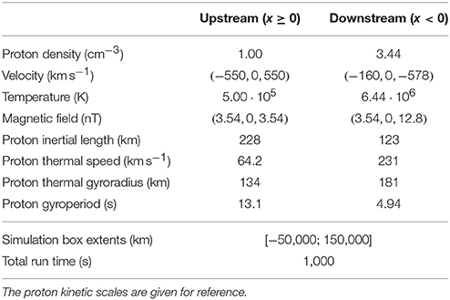
Table 1. Simulation parameters at initialization common to all runs, for the upstream (x ≥ 0) and downstream (x < 0) regions of the prescribed shock.
The simulations differ by a set of parameters as listed in Table 2. Two different Δx and three different Δv values are used, in runs with and without the Hall term in Ohm's law. A set of runs with fixed Δx, Δv and varying fmin is also performed. Additionally, a set of test-Vlasov runs are performed, that is runs in which only the proton velocity distribution function is propagated while the electric and magnetic fields are kept constant at their initial values. These test-Vlasov runs are conceptually equivalent to test-particle simulations in static fields performed with particle-based simulation methods. Table 3 gives the overview of the runs performed and the index used hereafter to refer to individual runs.
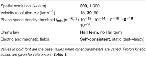
Table 2. Simulation parameter ranges tested between separate runs.
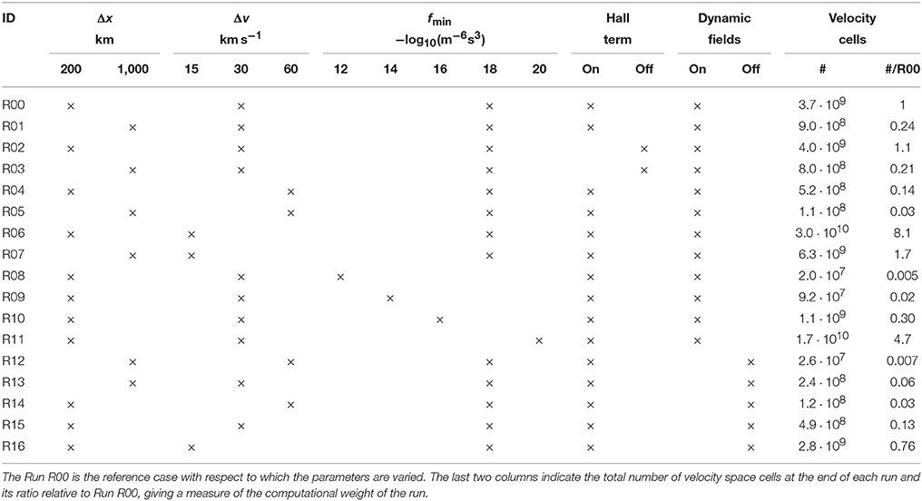
Table 3. Overview matrix of the runs performed.
The following standard visualization has been chosen in Figures 1, 3, 5, 7 to compare the output of all the runs performed. The ion number density is represented on a linear color scale ranging 0.8−4cm−3. Additionally, three-dimensional isosurface plots in velocity space of the phase space density at f = 10−15 m−6s3 (equivalent to a sphere with a radius of 5.0 proton thermal speeds in the upstream region at initialization) are shown at evenly-spaced locations along the box, marked with arrows. The velocity space coordinates are rotated such that the horizontal velocity axis is aligned with the instantaneous magnetic field and a cubic box of side length 3,000 km s−1 is included as a scale reference. For each figure showing this visualization of a set of runs, a corresponding animation showing the evolution of the system for the complete simulated time span is presented in the Supplemental data. The figures include 10 distribution plots per run, while the Supplemental data animations include 20 such plots.
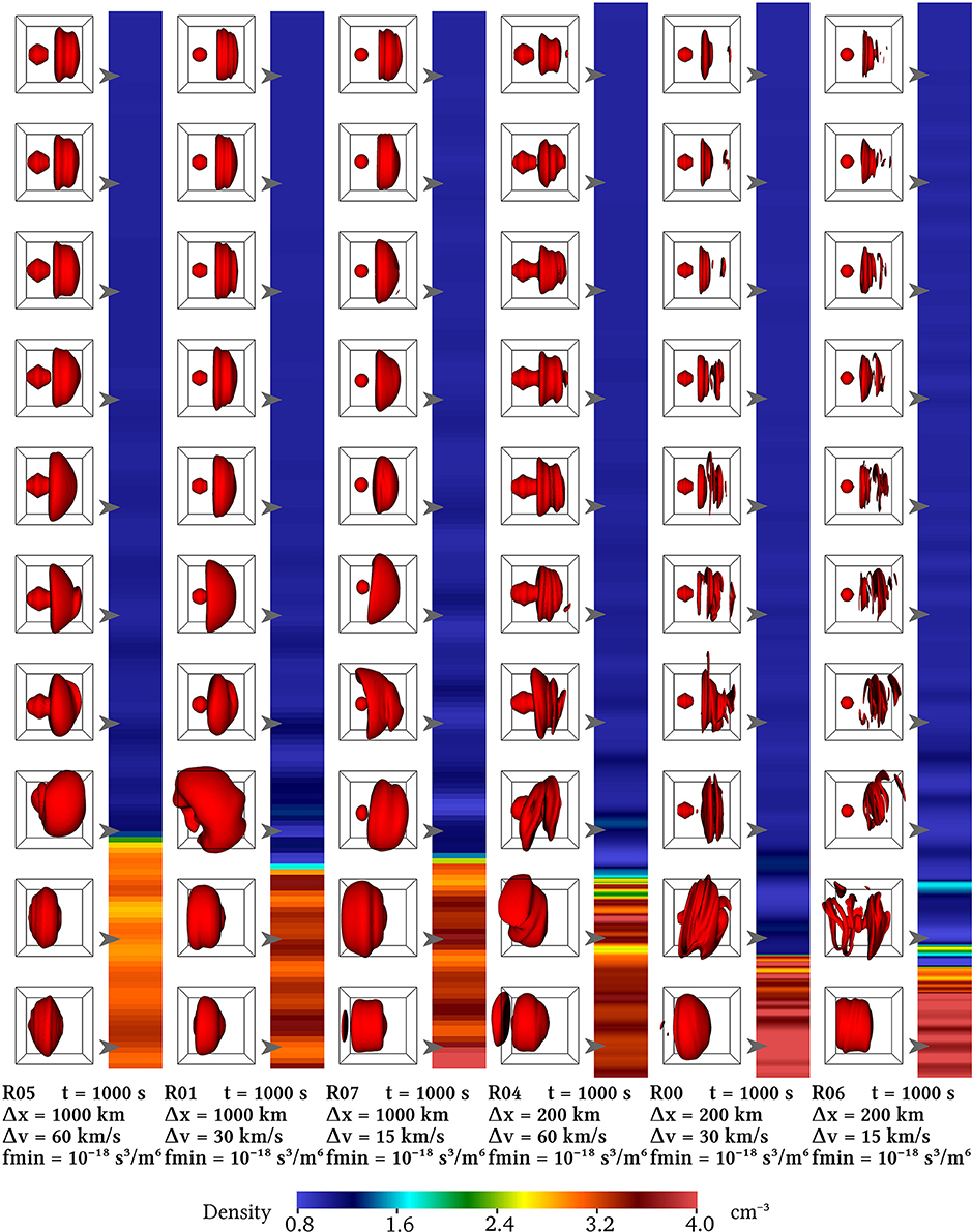
Figure 1. Runs R05, R01, R07, R04, R00, and R06 showing the effects of varying Δx and Δv, along with corresponding Supplemental data Animation A1. The profiles of ion number density and temperature are shown in Figure 2.
Given their identical initialization, all the runs are expected to evolve in a similar way which is summarized here. A high-density transient wave front travels through the downstream region until it exits the simulation box after approximately 350s. By that time, the reflected ion population forming the foreshock [44] has propagated upstream and the right-hand resonant beam instability grows, generating typical foreshock ULF waves [30, 45]. In the downstream region, the anisotropic heating of the ion population drives the 1D equivalent of mirror mode waves [47]. In the later phases of the simulation, the modulation of the upstream conditions by the foreshock ULF waves influences the evolution of the downstream region, with varying degrees of wave steepening observed in the upstream region.
The sets of Runs R05, R01, and R07 at Δx = 1,000 km and R04, R00, and R06 at Δx = 200km at their respective values of Δv = 60, 30, and 15kms−1 are first used to investigate the effects of improving Δx on the simulation. The final state of these runs is shown in Figure 1 and their entire sequence in Supplemental data Animation A1. Figure 2 shows the ion number density and temperature profiles for the final state of the same set of runs.
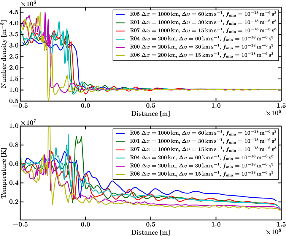
Figure 2. Number density and temperature profiles for Runs R05, R01, R07, R04, R00, and R06 showing the effects of varying Δx and Δv.
All runs shown in Figures 1, 2 exhibit the formation of foreshock and downstream waves. The comparison of the occurrence of steepened foreshock waves impinging on the shock front reveals that they reach similar amplitudes both at low and high Δx. However, the five-fold improvement in spatial resolution leads to a corresponding increase in the complexity and diversity of physical phenomena described by the runs. At Δx = 1,000 km, the foreshock and downstream waves are only approximately resolved by the grid, whereas Δx = 200km provides much better sampling of the dominant wavelengths. The finer resolution also allows shorter wavelength waves to be present and enables steeper gradients, for example at the steepened foreshock waves mentioned above or in the downstream waves visible in Figure 6. The study of the velocity distribution functions reveals that the spatial resolution has a large impact on their morphology. The finer detail of the spatial description leads to a greater complexity of the distributions at all Δv. The effects of varying Δx are further discussed in section 4.3.
The same set of Runs R05 and R04 (Δv = 60kms−1), R01 and R00 (Δv = 30kms−1), R07 and R06 (Δv = 15kms−1) is used to study the effect of varying Δv at both spatial resolution values Δx = 1,000 and 200km, with the same Figures 1, 2 as well as Supplemental data Animation A1.
At coarse Δx the improved Δv does not have major consequences when comparing Runs R01 and R07. The morphology of the foreshock and downstream waves as well as the velocity distributions are remarkably similar. More differences emerge at Δx = 200km, although Runs R00 and R06 are similar as well. Nevertheless, improving Δv has a fundamental impact on the diffusive properties of the model. It is best visible when considering the shape of the core solar wind population when it propagates from the upstream boundary toward the shock. The finer Δv is, the closer the core distribution is to the initial and nominal Maxwellian distribution throughout the upstream region. In comparison, decreasing the velocity resolution to Δv = 60kms−1 results in a significantly misshapen core distribution and a connected beam distribution. This has a distinct effect in over-representing the upstream temperature, as seen in Figure 2. This and further topics relating to the convergence of the simulation as a function of resolution are discussed further in section 4.3.
The sequence of runs R08, R09, R10, R00, and R11 allows to investigate the effect of the fmin threshold on the simulation, as each of these runs only differs by the value and 10−20m−6s3, respectively. These values correspond to a sphere with a radius of respectively 3.3, 4.5, 5.4, 6.2, and 6.9 proton thermal speeds in the upstream region at initialization. Figure 3 shows the final state of these runs, while Animation A2 in the Supplemental data shows the whole run sequences. Figure 4 shows the ion temperature profiles for the final state of these runs.
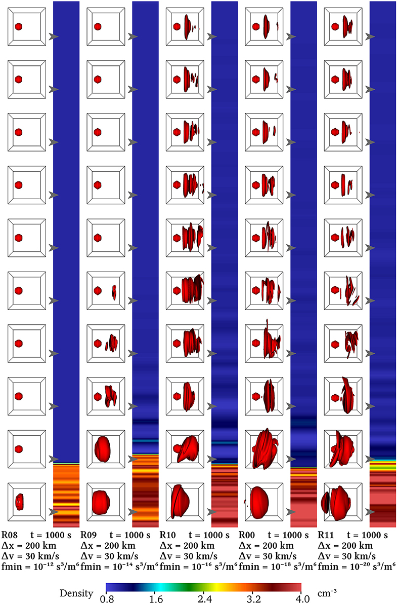
Figure 3. Runs R08, R09, R10, R00, and R11 showing the effect of decreasing fmin. For the given resolution parameters, the result of the shock simulation is converging, as can also be seen in the corresponding Supplemental data Animation A2 and Figure 4.
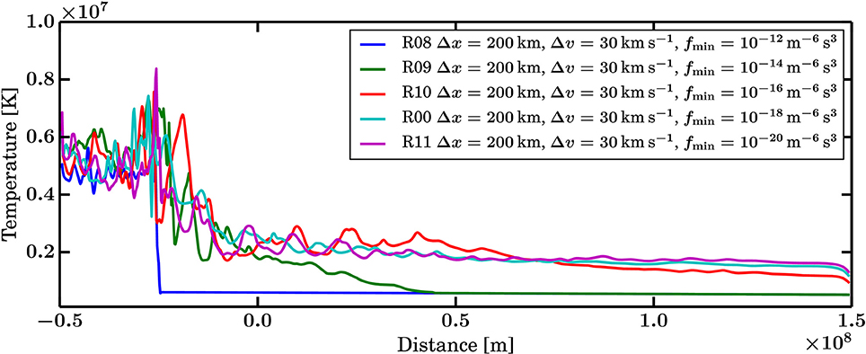
Figure 4. Temperature profiles for Runs R08, R09, R10, R00, and R11 showing the effect of decreasing fmin.
Although the isosurface plots of the velocity distribution function are all drawn at f = 10−15m−6s3 (sphere of 5.0 upstream proton thermal speeds at initialization), the velocity distributions are visible throughout Figure 3 and Animation A2. This stems from the fact that a layer of up to 8 velocity space cells is included beyond the last cells which have f > fmin, as explained by von Alfthan et al. [30] and Pfau-Kempf [41]. Within this layer, f is still propagated and it decreases steeply, so that it can reach values as low as the isosurface value even though that is well below fmin in R08 and R09. This is however not always the case, so that gaps can appear in the plots such as in the bottom left velocity distribution plot in R08 in Figure 3.
At the higher end of the range, R08 and R09 demonstrate the danger of setting a high value for fmin. This can lead to the complete loss of a significant fraction of the ions such as the foreshock ion beams reflected off the shock. Indeed the temperature profiles of Figure 4 show that for these two runs the temperature in the upstream region is constant at the core population value, whereas for the other cases the upstream temperature is strongly affected by the presence of the foreshock reflected ions. This is also evident in the near-total and total lack of foreshock waves in runs R09 and R08, respectively. R10, R00, and R11 are near and below the fmin values typically used in global magnetospheric simulations [44, 45, 47–49] and they result in similar states. In particular the latter R00 and R11 are very similar, as can be seen in Figure 4. Further implications of the choice of fmin are discussed in section 4.4.
Unsurprisingly, the inclusion of the Hall term in Ohm's law in the field solver has been shown to be instrumental in modeling wave modes and their dispersion beyond the plain magnetohydrodynamic behavior [50]. However, at the spatial resolutions which are currently computationally feasible for global magnetospheric simulations, the ion kinetic scales are not yet well-resolved, so that for example the whistler waves stemming from the Hall term inclusion are not resolved either. This means that the Hall term in Ohm's law only has a limited impact on the simulations performed in the present study. Comparing the Hall-less Runs R03 and R02 at Δx = 1,000 and 200km, respectively with their counterparts R01 and R00 in Figure 5, and Supplemental data Animation A3 shows that there is indeed no major differences with and without the Hall term in Ohm's law. This is also visible in Figure 6 which shows the profile of the magnetic field By component for these same runs.
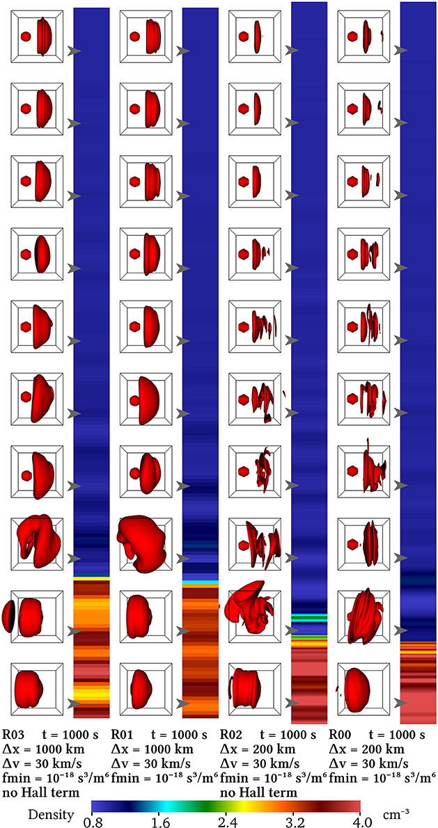
Figure 5. Runs R03, R01, R02, and R00 showing the effect of the Hall term in Ohm's law in the field solver. At these spatial resolutions, the Hall term effects are not expected to make a significant difference, as can also be seen in the corresponding Supplemental data Animation A3 and Figure 6.
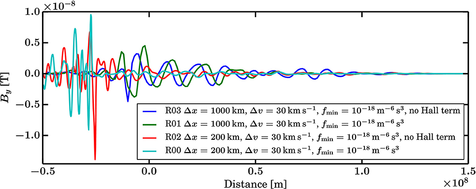
Figure 6. Magnetic field By profiles for Runs R03, R01, R02, and R00 showing the effect of the Hall term in Ohm's law in the field solver.
The runs R12, R13, R14, R15, and R16 are particular as they are performed in static fields. This means that after the initialization of the electric and magnetic fields, only f is propagated in time. It should be noted that due to the lack of electron physics and since the spatial resolutions are not sufficient, no particular structure or feature such as the cross-shock potential is present at the shock. These test-Vlasov runs are conceptually equivalent to test-particle simulations in static fields, where particles are subject to the Lorentz force but do not affect the fields in return. Runs R12 and R13 use Δv = 60 and 30kms−1 for the coarser Δx = 1,000 km and Runs R14, R15, and R16 use Δv = 60, 30, and 15kms−1 for the finer Δx = 200km. Their results are shown in Figure 7 and the corresponding Supplemental data Animation A4.
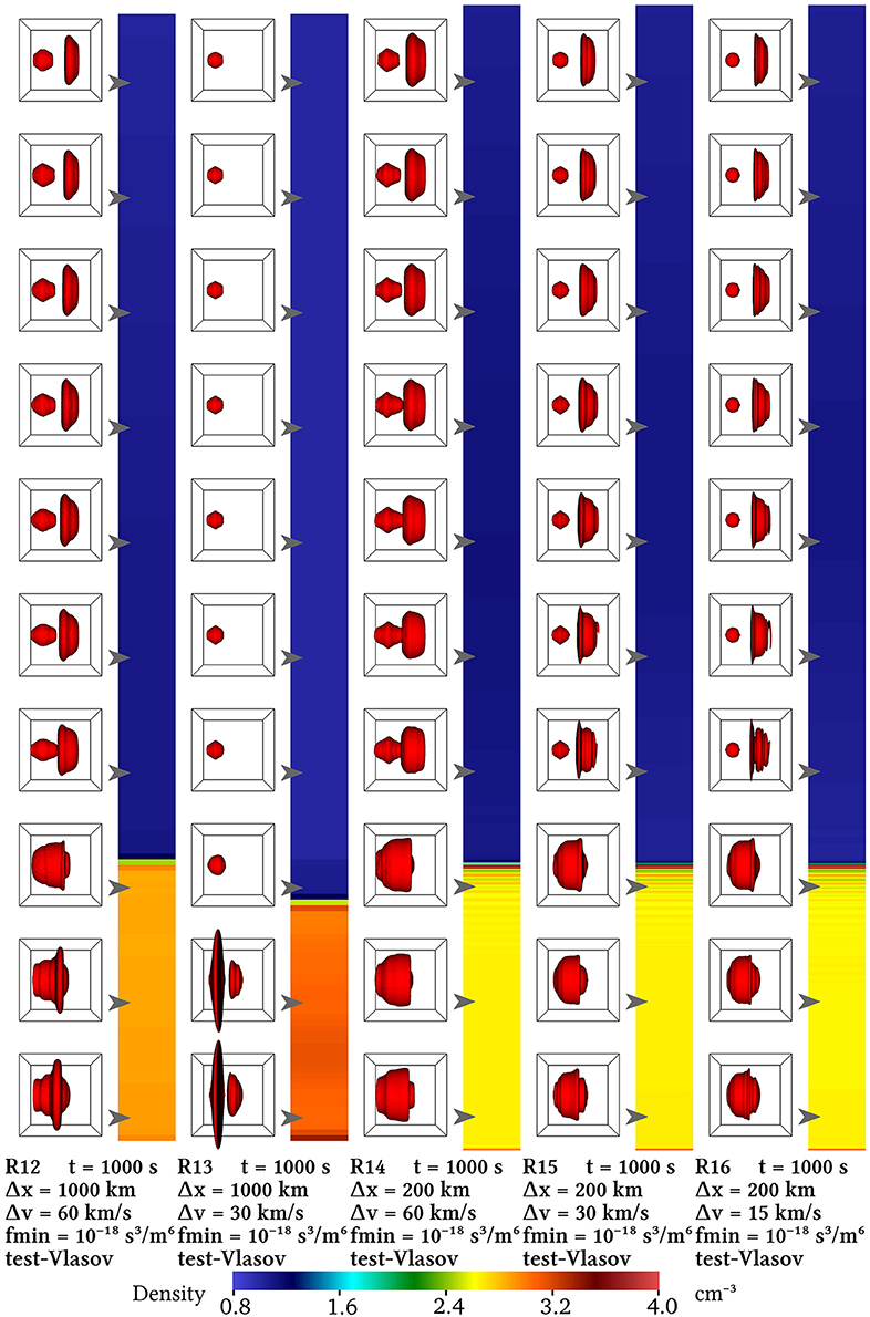
Figure 7. Runs R12, R13, R14, R15, and R16 in the test-Vlasov (static fields) configuration. Although the results do converge at finer Δx and Δv (R15, R16), the coarser cases (R12, R13, R14) give clearly unphysical results. Animation A4 is the corresponding Supplemental data.
Runs R15 and R16, with the finer resolution parameters, show convergence indeed. However, the three cases with coarser Δx and/or Δv (R12, R13, R14) clearly depart from the expected physical results, up to even losing the reflected foreshock ion population. In comparison, the equivalent self-consistent runs—respectively R05, R01, R04—do not fare as badly, as can be seen in Figure 1 and its corresponding Supplemental data Animation A1. Consequently, should Vlasiator be used in a test-Vlasov configuration, care has to be taken to ensure that the spatial and velocity resolutions are sufficiently good, and even better than for fully self-consistent runs.
In order to reduce the parameter space to be covered, the physical system chosen for this study is relatively simple, in particular with respect to global magnetospheric simulations which are the primary target in the development of Vlasiator. This simplification however makes it possible to explore a range of parameters at a fraction of the computational cost of global simulations. It also makes the visualization of the runs and their intercomparison less cumbersome.
The 1D-3V shock simulation simplifies shock reformation physics and excludes phenomena such as shock curvature and shock beading by design. Their analysis is well beyond the scope of the present study. A parameter study using magnetospheric simulations can be envisaged, but it involves a multitude of additional factors, regardless of the computational cost of such a simulation campaign. Such factors include possible feedback from the magnetopause [48, 49], or the consequences of the high magnetic fields of the geomagnetic dipole on the time propagation algorithm.
The shock parameters are chosen to be similar to those used in global magnetospheric simulations [44, 45, 47], in an effort to explain differences in the foreshock distribution functions. The discussion of this aspect is given in section 4.5 below.
The simulated shock is initialized in the de Hoffmann—Teller frame and according to the Rankine—Hugoniot conditions for a plasma shock, in an effort to keep the simulation domain size requirements minimal thanks to a stationary shock. The figures and Supplemental data animations show that this goal is approximately achieved, however it is clear that in all but the test-Vlasov runs the shock front moves downstream. Closer scrutiny reveals that the time when the shocks starts to recede, the receding speed, and the total distance the shock front travels during the simulation varies across the runs.
The explanation for this behavior is to be sought in the conditions for the stability of the shock. The Rankine–Hugoniot conditions are derived from the magnetohydrodynamic equations, which in turn imply a set of assumptions regarding the modeled plasma. In particular, the assumption that the plasma can be described by a single, isotropic Maxwellian particle population is not valid in the present hybrid-Vlasov simulations. As a result, the Rankine–Hugoniot conditions are violated to a certain degree due to the inherently kinetic description of the shock in Vlasiator.
The systematic analysis of the deviations from each of the components of the Rankine–Hugoniot jump conditions, performed for each of the runs in this study, confirms what the physical intuition regarding the setup suggests. The recession of the shock is mostly due to an imbalance in the conservation of the longitudinal momentum of the plasma. Indeed the reflection of the foreshock ions off the shock is a kinetic phenomenon not accounted for in the magnetohydrodynamic description. Another discrepancy with respect to the magnetohydrodynamic theory is the loss of isotropy/gyrotropy of the velocity distribution. It leads to the violation of the coplanarity theorem which stipulates that the upstream and downstream magnetic field and velocity vectors are coplanar across a magnetohydrodynamic shock. As a consequence of this violation, some momentum is transferred into the out-of-plane direction.
The dependency of the shock position on the “amount” of kinetic physics can be appreciated in Figure 1 and Supplemental data Animation A1 as well as in the density profiles shown in Figure 2. The “more” kinetic Runs R00 and R06 (as discussed further in section 4.3) are deviating most from the initial magnetohydrodynamic equilibrium position. The comparison with Figure 3 and Supplemental data Animation A2 shows that Δx and Δv have a stronger impact on the shock position than fmin in this setting, whereas Figure 5 and Supplemental data Animation A3 suggest that the Hall term does not have a significant impact at the Δx used. The resolution and fmin are discussed further in sections 4.3 and 4.4, respectively. The recession of the shock in the runs of this study is therefore no more than a confirmation of the kinetic nature of the simulations, departing from the simpler magnetohydrodynamic theory used to derive the initial shock stability conditions.
The quality and trustworthiness of a numerical model is always and naturally assessed in terms of its convergence toward a reference or true result, both in verification against another previously established model or theory [e.g., 49, 50, in the case of Vlasiator] and validation against experimental data [e.g., 44, 45]. The parameter space covered by the runs in this work gives an insight into the convergence properties of Vlasiator with respect to Δx, Δv, and fmin. The former two are discussed here, the latter is discussed in section 4.4.
The set of Runs R05, R01, R07 and R04, R00, R06 presented in sections 3.1 and 3.2 as well as Figures 1, 2 and Supplemental data Animation A1 is designed to investigate the convergence as a function of Δx and Δv. Only two values of Δx are used, which is insufficient to claim that the results converge. Additionally, the spatial resolution does not yet allow to properly resolve the ion kinetic scales (ion gyroradius and inertial length), which are however of physical relevance in a hybrid model including the Hall term in Ohm's law. As an illustration, the magnetic field By component profiles in Figure 6 show that neither the amplitude nor the wavelength of the waves are similar when comparing both values of Δx, indicating a lack of convergence in this respect. Yet, as stated before, one goal of this study is to provide a reference for existing and future global magnetospheric simulations. Thus, for the sake of comparison to existing magnetospheric simulations and to stay within realistic computation times for such a study, the present choice of resolution parameters is made.
The comparison of Runs R00 and R06 shows that for Δx = 200km, improving Δv from 30 to 15km s−1 yields a very similar result in terms of shock position, upstream, and downstream waves and suprathermal ion distributions, while Run R04 at Δv = 60km s−1 exhibits less complex distributions and a shock position closer to the magnetohydrodynamic rest position. In contrast, at Δx = 1,000 km the two Runs R01 and R07 at finer Δv do feature more complex waves than the coarsest Run R05 but the morphology of the velocity distributions does not vary much in these three runs. Hence the conclusion that Δx and Δv have to be considered together, as improving only Δv at coarse Δx does not produce as complex kinetic physics as a moderate improvement of Δv coupled with an improved Δx does.
The adequate choice of Δx with respect to the length scales of the modeled phenomena is particularly important in studies involving plasma instabilities and their growth. Indeed as was already pointed out in previous work with Vlasiator [30], the wave number and growth rate of the fastest growing mode of a given instability is influenced by the total size of the box and the number of grid points resolving the wave. The systematic study of plasma beam instabilities in the relativistic regime by Shalaby et al. [52] shows that even in the linear growth phase the resolution and simulation domain extents have to be sufficient in order to cover the spectral support of the instability and obtain the correct growth rate and wave number of the fastest-growing mode. While the detail of instabilities is not investigated here, this factor has to be taken into account when interpreting such instabilities in simulation results or defining the parameters of new simulations.
A major discussion point on the impact of resolution in Vlasiator simulations pertains to the numerical diffusive properties of the model. As reported elsewhere [30, 41, 45], the propagation algorithm is split in three parts. In the current version of the solvers the acceleration of f is solved to fifth order in Δv, the translation of f is solved to third order in Δx and the field propagation is solved to second order in Δx. The time stepping is of second order due to the Strang splitting scheme applied and thanks to the second-order Runge—Kutta stepping of the field solver. Therefore, Δx affects the amount of numerical diffusion in translation, for instance a finer resolution allows to better preserve steep gradients such as shocks and steepened waves, as visible for example in Figure 6. Similarly Δv affects the level of diffusion in velocity space. This is particularly evident when observing the solar wind core distribution in Figure 1 and Supplemental data Animation A1. At coarse Δv the initially isotropic and relatively cold Maxwellian distribution is distorted into a gyrotropic but clearly non-spherical shape, and its width increases during propagation toward the shock. This directly affects the moments of f such as the ion temperature, which increases due to this numerical diffusion. At the intermediate and finer Δv values the diffusion is much better kept at bay and the solar wind core population remains similar to the nominal distribution. The analysis of the temperature profiles shown in Figure 2 confirms this behavior, as only Runs R00 and R06 converge to a similar state, whereas the coarser runs exhibit higher temperatures and stronger temperature perturbations in the upstream region due to the diffusion. Finally the resolution parameters have an impact on the length of the time steps that the solver can take. Finer resolutions require shorter time steps as signals propagating with advection and plasma wave speeds must not travel more than one cell width per time step. Therefore, a larger number of steps has to be taken in order to reach the same simulated time, which increases the level of diffusion. The runs presented here however show that sufficient Δx and Δv are required to obtain physical results at kinetic scales, be it at the cost of shorter and more numerous time steps, in addition to the higher cost of the larger number of grid points.
The runs presented in section 3.3 investigate the convergence of the simulation with respect to the value of fmin. For obvious reasons the sparse velocity space strategy violates the conservation of f and its moments (density, momentum, pressure, etc.) inherent to the Vlasov equation. While this permits enticing computational gains, the higher the level of fmin, the more drastic the losses of f become as illustrated in Figure 3 and Supplemental data Animation A2. The temperature profiles of Figure 4 show the same result. For both Runs R08 and R09 with highest fmin the ion temperature shows that the foreshock beam population is no longer present in the upstream region. This variable is very sensitive to the presence of a fast ion beam.
The first aspect to consider is the accurate description of the prescribed initial and boundary conditions. The values of fmin and Δv have to be set such that the moments of f have the desired accuracy. Coarse parameters lead to a worse accuracy of the moments independently of the subsequent numerical diffusion occurring during propagation.
The second aspect to consider is the quality of mass conservation and the preservation of desired features such as more tenuous ion beams. By definition, the lower the threshold is set, the more low-density features in phase-space are preserved which could have a dynamic significance. With parameters such as Run R08 or R09 even the ion foreshock beams have densities lower than the threshold, leading to their loss, corresponding to a mass loss of the order of 1% of the total mass. Higher moments are even more affected, as the high-velocity tails of the distributions are the first to be truncated due to a high fmin value. For most applications, such values of fmin are likely insufficient.
Nevertheless, the computational cost of decreasing fmin is steep. As shown in the last two columns of Table 3, the number of velocity space cells, that is the number of 1D-3V phase space sampling points in the Runs R08, R09, R10, R00, and R11 is respectively 2.0 · 107, 9.2 · 107, 1.1 · 109, 3.7 · 109, and 1.7 · 1010, which gives an indication of the evolution of the computational cost as a function of fmin in these runs.
Of the simulations presented here, R00 and R11 do converge toward a similar state. It is however not excluded that dynamically significant but more tenuous parts of the velocity distributions have been discarded due to the sparse velocity space mechanism. Hence, the choice of fmin has to be a trade-off between the degree of physical accuracy and the computational weight of the simulation. Future avenues of development include a more adaptive determination of fmin based on, for instance, the local thermal velocity of the distribution, or adaptive mesh refinement in velocity space, both of which could allow the tracking of low-density phase-space features at an affordable computational cost.
The shock parameters in this study are similar to those used in global magnetospheric simulations [44, 45, 47]. The early simulation [44] exhibits well-identified velocity distribution types matching spacecraft observations. However the foreshock ion distributions in the latter simulations presented by Palmroth et al. [45] and in particular Hoilijoki et al. [47] are more complex and a classification according to the types presented by Kempf et al. [44] is not possible.
There are numerous differences between these two generations of simulations. The Vlasov solver evolved from a Eulerian propagator to the current semi-Lagrangian one, decreasing the overall numerical diffusivity of the model. This and further code improvements enabled significant improvements in Δx (from 850 to 227km) while relaxing the requirements on Δv (from 20 to 30kms−1) but still improving the diffusive properties of the solver. The solar wind and shock parameters, especially the Alfvénic Mach number, are not identical. Closer inspection reveals that, due to a combination of the above, the bow shock structure is much smoother in the former simulation than in the latter, where shock beading occurs albeit close to the grid resolution.
The runs presented here demonstrate that, notwithstanding all the other differences, the improved Δx alone is sufficient to achieve the quantum leap seen in the ion velocity distribution complexity. This is evident when comparing the velocity distributions in Runs R01 and R00 in Figure 1 and Supplemental data Animation A1 and noticing that the step from coarse to fine Δx (Run R01 to R00) has a much stronger impact than the step to a finer Δv (Run R00 to R06).
The computational weight of the field solver in Vlasiator scales linearly with the number of spatial cells, thus with (Δx)−1. However, the computational cost is dominated by the Vlasov solver's translation and acceleration operations, which scale approximately linearly with the number of velocity space cells, thus with (Δv)−3. The memory consumption is also dominated by the velocity space and it scales as (Δv)−3. These approximate scalings are reflected in the total number of velocity cells as is visible in Table 3. R01 and R03 at Δx = 1,000 km have close to 5 times less velocity cells than R00 and R02 with Δx = 200km, whereas R06 (Δv = 15kms−1) has about 8 = 23 times more cells than R00 (Δv = 30kms−1). The scaling of the number of velocity cells with fmin is not linear, as shown in section 4.4, but very steep so that lowering fmin comes at a large computational cost.
In addition to the memory usage and the raw number of computations per step, the computational cost of a run scales inversely with the length of the time steps. That in turn is affected by Δx, but also by the physical parameters simulated. For example, higher magnetic fields result in shorter allowed gyration steps and limit the length of the admissible field solver time steps, as do lower densities in the latter case. These combined effects however cannot be controlled directly by setting simulation parameters. Additionally the length of the time step is adapted dynamically during a run.
Lastly, the computational weight is dependent on the architecture the code is run on, and on the parallelization parameters. Velocity space computations greatly benefit from vectorization, while the number of threads per process and the overall number of processes or computation nodes used affect the quality of the load balancing and the efficiency of inter-process communication.
The overall computational weight of a run is the result of a number of parameters. The interdependence of these parameters means that the effective computational cost of a simulation run cannot be determined exactly beforehand. The parameter most affected by Δx, Δv, and fmin is the number of 1D-3V phase space sampling points, affecting mostly the Vlasov solver. The detailed study of the computational efficiency of Vlasiator is however beyond the scope of this work. It should also be noted that as with any simulation software, new improvements to numerical efficiency are constantly being implemented.
It would be futile to state here explicit quantitative recommendations in terms of Δx, Δv, and fmin for future applications of Vlasiator or any other hybrid-Vlasov model. Their choice is dictated by a range of technical and physical requirements, as evidenced in the previous sections.
First of all, the resolutions have to ensure that the quality of the propagation in terms of the conservation of the moments of f in particular meets quality criteria sufficient for the targeted modeling. In that sense, Δv should ensure that for example the thermal width of the coldest relevant component—the upstream inflowing population in this study—is well-resolved, that is resolved by at least a few velocity cells. Likewise, fmin should ensure mass conservation to required accuracy. This means covering an amplitude of at least 5–6 orders of magnitude of phase space density in the runs presented here. In other cases, like studies of particle acceleration at shocks, a larger range of f is required in order to allow the acceleration process to proceed from tenuous, high-energy accelerated ions to a full-fledged tail of the ion energy spectrum.
The next step is to evaluate which spatial scales are relevant to the problem and must be well-resolved. As an extreme example, the electron gyroradius and the Debye length are not relevant in the hybrid-Vlasov context. The ion kinetic scales (ion gyroradius and inertial length), however, are potentially of interest, even though this and previous work shows that even with under-resolved kinetic scales Vlasiator produces kinetic phenomena. Unlike the Δv and fmin parameters, a coarser Δx does not directly affect the conservation of moments of f but it can reduce the range of physical phenomena modeled in the simulation.
Finally, the likely most stringent factor to determine simulation parameters is the availability and manageability of computational resources. The runs in this study can be performed using on the order of ~10 to ~5,000 node-hours (excluding post-processing) on a modern supercomputer, the upper limit being reached for runs with a fine Δv and low fmin like Runs R06 and R11. Large-scale magnetospheric simulations, on the other hand, require investments on the scale of 105 − 106 node-hours despite significant trade-offs being made in terms of the dimensionality of the problem and the resolution of kinetic scales.
Therefore, a balance of physical resolutions compounded by the computational feasibility has to be struck whenever a new setup is considered. The results of this study also show that care has to be exercised when trying to extrapolate from low-resolution test setups toward large-scale production runs. A synthetic overview of the parameters, their requirements as well as their major advantages and disadvantages is given in Table 4.
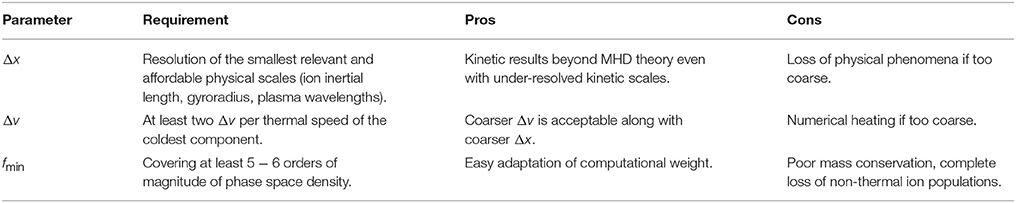
Table 4. Minimum requirements for Δx, Δv, and fmin along with related major advantages and disadvantages in hybrid-Vlasov simulations with Vlasiator.
A set of 1D-3V simulations of a shock with parameters similar to the terrestrial bow shock was performed using the hybrid-Vlasov model Vlasiator. The set was designed to investigate the effects of varying the spatial and velocity resolution, the minimum phase space density threshold and including or excluding the Hall term in Ohm's law in the field solver. Test-Vlasov runs in which the electric and magnetic fields are kept static were also performed for comparison.
The results presented highlight specificities of the hybrid-Vlasov method, which only relatively recently became affordable for large-scale plasma modeling. Therefore, this work is a benchmark for existing and future large-scale simulations performed with Vlasiator. It also documents the effects the various investigated parameters can have on the behavior of the algorithm.
In agreement with previously published global magnetospheric simulations performed with Vlasiator [44, 45, 47], it appears that it is not necessary to fully resolve ion kinetic spatial scales in order to obtain kinetic results departing from magnetohydrodynamic theory. However, the choice of resolution and minimum phase space threshold values must take into account the physical phenomena to be modeled as well as the momentum conservation properties of the algorithm. It is shown in particular that the spatial and velocity resolutions should be increased together rather than favoring either one. The resulting choice of parameters must ensure that targeted quality criteria are met while remaining within acceptable limits of computational weight.
YP-K designed the study following discussions with and a visit to Bertrand Lembège at Laboratoire ATmosphères, Milieux, Observations Spatiales (LATMOS), Université de Versailles Saint-Quentin-en-Yvelines, Guyancourt, France, as well as discussions with all co-authors. YP-K performed the simulations and their post-processing with the help of MB and UG. All co-authors contributed to the analysis of the results and commented extensively on the manuscript during its writing by YP-K.
The authors acknowledge support of the Academy of Finland through grant 267144 and the Finnish Centre of Excellence in Research of Sustainable Space (Academy of Finland grant number 312351), as well as the European Research Council Consolidator through grant 682068-PRESTISSIMO. Vlasiator (http://www.physics.helsinki.fi/vlasiator) has also been developed with the support of the Academy of Finland and the European Research Council Starting grant 200141-QuESpace. YP-K acknowledges financial support by the Magnus Ehrnrooth foundation for a scientific visit to Bertrand Lembège at LATMOS, UVSQ, Guyancourt, France and by the Finnish Social Insurance Institution of Finland during his parental leave. The work of LT was supported by a Marie Skłodowska-Curie Individual Fellowship (#704681).
The authors declare that the research was conducted in the absence of any commercial or financial relationships that could be construed as a potential conflict of interest.
The reviewer VF and handling editor declared their shared affiliation.
YP-K acknowledges discussions with Bertrand Lembège.
We acknowledge the PRACE Tier-0 14th call grant 2016153521 for the use of Marconi at CINECA, Italy and CSC – Finnish IT Center for Science for the use of Sisu at CSC, Finland.
The source code is available on the GitHub platform (http://github.com/fmihpc/vlasiator), the code version used in this work corresponds to the commit tag 09ea808d with the modification #define MAX_BLOCKS_PER_DIM 268 in the file common.h.
The GNU Parallel tool is used in many steps for the production of the Supplemental data animations [53].
The Supplementary Material for this article can be found online at: https://www.frontiersin.org/articles/10.3389/fphy.2018.00044/full#supplementary-material
A set of animations is provided as Supplemental data. Each animation corresponds to a figure and their design is explained in section 2.3.
1. Supplemental data Animation A1 corresponding to Figure 1.
2. Supplemental data Animation A2 corresponding to Figure 3.
3. Supplemental data Animation A3 corresponding to Figure 5.
4. Supplemental data Animation A4 corresponding to Figure 7.
1. Fisher DM, Rogers BN. Two-fluid biasing simulations of the large plasma device. Phys Plasmas (2017) 24:022303. doi: 10.1063/1.4975616
2. Görler T, Lapillonne X, Brunner S, Dannert T, Jenko F, Merz F, et al. The global version of the gyrokinetic turbulence code GENE. J Comput Phys. (2011) 230:7053–71. doi: 10.1016/j.jcp.2011.05.034
3. Vaivads A, Retinò A, Soucek J, Khotyaintsev YV, Valentini F, Escoubet CP, et al. Turbulence Heating ObserveR–satellite mission proposal. J Plasma Phys. (2016) 82:90582050. doi: 10.1017/S0022377816000775
4. Innocenti ME, Cazzola E, Mistry R, Eastwood JP, Goldman MV, Newman DL, et al. Switch-off slow shock/rotational discontinuity structures in collisionless magnetic reconnection: what to look for in satellite observations. Geophys Res Lett. (2017) 44:3447–55. doi: 10.1002/2017GL073092
5. Bourdin PA, Bingert S, Peter H. Scaling laws of coronal loops compared to a 3D MHD model of an active region. A&A (2016) 589:A86. doi: 10.1051/0004-6361/201525840
6. Kempf A, Kilian P, Spanier F. Energy loss in intergalactic pair beams: particle-in-cell simulation. A&A (2016) 585:A132. doi: 10.1051/0004-6361/201527521
7. Büchner J, Dum C, Scholer M. (ed.). Space Plasma Simulation. Vol. 615 of Lecture Notes in Physics. Berlin; Heidelberg: Springer Verlag (2003).
8. Hockney RW, Eastwood JW. Computer Simulation Using Particles. New York, NY; London: CRC Press (1988).
9. Birdsall CK, Langdon AB. Plasma Physics via Computer Simulation. Series in Plasma Physics. New York, NY; London: CRC Press (2004).
10. Omidi N, Blanco-Cano X, Russell CT. Macrostructure of collisionless bow shocks: 1. Scale lengths. J Geophys Res. (2005) 110:A12212. doi: 10.1029/2005JA011169
11. Blanco-Cano X, Omidi N, Russell CT. Macrostructure of collisionless bow shocks: 2. ULF waves in the foreshock and magnetosheath. J Geophys Res. (2006) 111:10205. doi: 10.1029/2005JA011421
12. Markidis S, Lapenta G, Rizwan-uddin. Multi-scale simulations of plasma with iPIC3D. Math Comput Simul. (2010) 80:1509–19. doi: 10.1016/j.matcom.2009.08.038
13. Daughton W, Roytershteyn V, Karimabadi H, Yin L, Albright BJ, Bergen B, et al. Role of electron physics in the development of turbulent magnetic reconnection in collisionless plasmas. Nat Phys. (2011) 7:539–42. doi: 10.1038/nphys1965
14. Savoini P, Lembège B, Stienlet J. On the origin of the quasi-perpendicular ion foreshock: full-particle simulations. J Geophys Res. (2013) 118:1132–45. doi: 10.1002/jgra.50158
15. Karimabadi H, Roytershteyn V, Vu HX, Omelchenko YA, Scudder J, Daughton W, et al. The link between shocks, turbulence, and magnetic reconnection in collisionless plasmas. Phys Plasmas (2014) 21:062308. doi: 10.1063/1.4882875
16. Kempf A, Kilian P, Ganse U, Schreiner C, Spanier F. PICPANTHER: a simple, concise implementation of the relativistic moment implicit particle-in-cell method. Comput Phys Commun. (2015) 188:198–207. doi: 10.1016/j.cpc.2014.11.010
17. Lu S, Lu Q, Lin Y, Wang X, Ge Y, Wang R, et al. Dipolarization fronts as earthward propagating flux ropes: a three-dimensional global hybrid simulation. J Geophys Res. (2015) 120:6286–300. doi: 10.1002/2015JA021213
18. Hao Y, Gao X, Lu Q, Huang C, Wang R, Wang S. Reformation of rippled quasi-parallel shocks: 2-D hybrid simulations. J Geophys Res. (2017) 122:6385–96. doi: 10.1002/2017JA024234
19. Lin Y, Wing S, Johnson JR, Wang XY, Perez JD, Cheng L. Formation and transport of entropy structures in the magnetotail simulated with a 3-D global hybrid code. Geophys Res Lett. (2017) 44:5892–9. doi: 10.1002/2017GL073957
20. Arslanbekov RR, Kolobov VI, Frolova AA. Kinetic solvers with adaptive mesh in phase space. Phys Rev E (2013) 88:063301. doi: 10.1103/PhysRevE.88.063301
21. Sonnendrücker E, Roche J, Bertrand P, Ghizzo A. The Semi-Lagrangian method for the numerical resolution of the Vlasov equation. J Comput Phys. (1999) 149:201–20. doi: 10.1006/jcph.1998.6148
22. Filbet F, Sonnendrücker E, Bertrand P. Conservative numerical schemes for the Vlasov equation. J Comput Phys. (2001) 172:166–87. doi: 10.1006/jcph.2001.6818
23. Besse N, Sonnendrücker E. Semi-Lagrangian schemes for the Vlasov equation on an unstructured mesh of phase space. J Comput Phys. (2003) 191:341–76. doi: 10.1016/S0021-9991(03)00318-8
24. Nunn D. Vlasov hybrid simulation—an efficient and stable algorithm for the numerical simulation of collision-free plasma. Trans Theory Stat Phys. (2005) 34:151–71. doi: 10.1080/00411450500255518
25. Schmitz H, Grauer R. Darwin–Vlasov simulations of magnetised plasmas. J Comput Phys. (2006) 214:738–56. doi: 10.1016/j.jcp.2005.10.013
26. Valentini F, Trávníček P, Califano F, Hellinger P, Mangeney A. A hybrid-Vlasov model based on the current advance method for the simulation of collisionless magnetized plasma. J Comput Phys. (2007) 225:753–70. doi: 10.1016/j.jcp.2007.01.001
27. Qiu JM, Christlieb A. A conservative high order semi-Lagrangian WENO method for the Vlasov equation. J Comput Phys. (2010) 229:1130–49. doi: 10.1016/j.jcp.2009.10.016
28. Eliasson, B Numerical simulations of the Fourier-transformed Vlasov-Maxwell system in higher dimensions–theory and applications. Transport Theory Stat Phys. (2011) 39:387–465. doi: 10.1080/00411450.2011.563711
29. Umeda T, Fukazawa K, Nariyuki Y, Ogino T. A scalable full-electromagnetic Vlasov solver for cross-scale coupling in space plasma. IEEE Trans Plasma Sci. (2012) 40:1421–8. doi: 10.1109/TPS.2012.2188141
30. von Alfthan S, Pokhotelov D, Kempf Y, Hoilijoki S, Honkonen I, Sandroos A, et al. Vlasiator: first global hybrid-Vlasov simulations of Earth's foreshock and magnetosheath. J Atmos Sol-Terr Phys. (2014) 120:24–35. doi: 10.1016/j.jastp.2014.08.012
31. Tronci C, Tassi E, Camporeale E, Morrison PJ. Hybrid Vlasov-MHD models: Hamiltonian vs. non-Hamiltonian. Plasma Phys Controll Fus. (2014) 56:095008. doi: 10.1088/0741-3335/56/9/095008
32. Kormann K. A Semi-Lagrangian Vlasov solver in tensor train format. SIAM J Sci Comput. (2015) 37:B613–32. doi: 10.1137/140971270
33. Cerri SS, Servidio S, Califano F. Kinetic cascade in solar-wind turbulence: 3D3V hybrid-kinetic simulations with electron inertia. Astrophys J Lett. (2017) 846:L18. doi: 10.3847/2041-8213/aa87b0
34. Sarrat M, Ghizzo A, Del Sarto D, Serrat L. Parallel implementation of a relativistic semi-Lagrangian Vlasov-Maxwell solver. Eur Phys J D (2017) 71:271. doi: 10.1140/epjd/e2017-80188-4
35. Wettervik BS, DuBois TC, Siminos E, Fülöp T. Relativistic Vlasov-Maxwell modelling using finite volumes and adaptive mesh refinement. Eur Phys J D (2017) 71:157. doi: 10.1140/epjd/e2017-80102-2
36. Juno J, Hakim A, TenBarge J, Shi E, Dorland W. Discontinuous Galerkin algorithms for fully kinetic plasmas. J Comput Phys. (2018) 353:110–47. doi: 10.1016/j.jcp.2017.10.009
37. Sydora RD. Low-noise electromagnetic and relativistic particle-in-cell plasma simulation models. J Comput Appl Math. (1999) 109:243–59. doi: 10.1016/S0377-0427(99)00161-2
38. Nevins WM, Hammett GW, Dimits AM, Dorland W, Shumaker DE. Discrete particle noise in particle-in-cell simulations of plasma microturbulence. Phys Plasmas (2005) 12:122305. doi: 10.1063/1.2118729
39. Holod I, Lin Z. Statistical analysis of fluctuations and noise-driven transport in particle-in-cell simulations of plasma turbulence. Phys Plasmas (2007) 14:032306. doi: 10.1063/1.2673002
40. Palmroth M, Honkonen I, Sandroos A, Kempf Y, von Alfthan S, Pokhotelov D. Preliminary testing of global hybrid-Vlasov simulation: magnetosheath and cusps under northward interplanetary magnetic field. J Atmos Solar-Terrest Phys. (2013) 99:41–6. doi: 10.1016/j.jastp.2012.09.013
41. Pfau-Kempf, Y Vlasiator – From Local to Global Magnetospheric Hybrid-Vlasov Simulations. Finnish Meteorological Institute Contributions (2016).
42. Hoilijoki S. Simulations of Solar Wind – Magnetosheath – Magnetopause Interactions. Finnish Meteorological Institute Contributions (2017).
43. Pokhotelov D, von Alfthan S, Kempf Y, Vainio R, Koskinen HEJ, Palmroth M. Ion distributions upstream and downstream of the Earth's bow shock: first results from Vlasiator. Ann Geophys. (2013) 31:2207–12. doi: 10.5194/angeo-31-2207-2013
44. Kempf Y, Pokhotelov D, Gutynska O, Wilson III LB, Walsh BM, von Alfthan S, et al. Ion distributions in the Earth's foreshock: hybrid-Vlasov simulation and THEMIS observations. J Geophys Res. (2015) 120:3684–701. doi: 10.1002/2014JA020519
45. Palmroth M, Archer M, Vainio R, Hietala H, Pfau-Kempf Y, Hoilijoki S, et al. ULF foreshock under radial IMF: THEMIS observations and global kinetic simulation Vlasiator results compared. J Geophys Res. (2015) 120:8782–98. doi: 10.1002/2015JA021526
46. Sandroos A, von Alfthan S, Hoilijoki S, Honkonen I, Kempf Y, Pokhotelov D, et al. “Vlasiator: global kinetic magnetospheric modeling tool,” in Numerical Modeling of Space Plasma Flows ASTRONUM-2014, Vol. 498 of Astronomical Society of the Pacific Conference Series (2015). p. 222.
47. Hoilijoki S, Palmroth M, Walsh BM, Pfau-Kempf Y, von Alfthan S, Ganse U, et al. Mirror modes in the Earth's magnetosheath: results from a global hybrid-Vlasov simulation. J Geophys Res. (2016) 121:4191–204. doi: 10.1002/2015JA022026
48. Pfau-Kempf Y, Hietala H, Milan SE, Juusola L, Hoilijoki S, Ganse U, et al. Evidence for transient, local ion foreshocks caused by dayside magnetopause reconnection. Ann Geophys. (2016) 34:943–59. doi: 10.5194/angeo-34-943-2016
49. Hoilijoki S, Ganse U, Pfau-Kempf Y, Cassak PA, Walsh BM, Hietala H, et al. Reconnection rates and X-line motion at the magnetopause: global 2D-3V hybrid-Vlasov simulation results. J Geophys Res. (2017) 122:2877–88. doi: 10.1002/2016JA023709
50. Kempf Y, Pokhotelov D, von Alfthan S, Vaivads A, Palmroth M, Koskinen HEJ. Wave dispersion in the hybrid-Vlasov model: verification of Vlasiator. Phys Plasmas (2013) 20:112114. doi: 10.1063/1.4835315
Keywords: plasma physics, kinetic modeling, hybrid-Vlasov modeling, Vlasiator, collisionless shock, foreshock, velocity distribution function, resolution
Citation: Pfau-Kempf Y, Battarbee M, Ganse U, Hoilijoki S, Turc L, von Alfthan S, Vainio R and Palmroth M (2018) On the Importance of Spatial and Velocity Resolution in the Hybrid-Vlasov Modeling of Collisionless Shocks. Front. Phys. 6:44. doi: 10.3389/fphy.2018.00044
Received: 15 February 2018; Accepted: 30 April 2018;
Published: 17 May 2018.
Edited by:
Vladimir I. Kolobov, CFD Research Corporation, United StatesReviewed by:
Ashkbiz Danehkar, Harvard-Smithsonian Center for Astrophysics, United StatesCopyright © 2018 Pfau-Kempf, Battarbee, Ganse, Hoilijoki, Turc, von Alfthan, Vainio and Palmroth. This is an open-access article distributed under the terms of the Creative Commons Attribution License (CC BY). The use, distribution or reproduction in other forums is permitted, provided the original author(s) and the copyright owner are credited and that the original publication in this journal is cited, in accordance with accepted academic practice. No use, distribution or reproduction is permitted which does not comply with these terms.
*Correspondence: Yann Pfau-Kempf, eWFubi5rZW1wZkBoZWxzaW5raS5maQ==
Disclaimer: All claims expressed in this article are solely those of the authors and do not necessarily represent those of their affiliated organizations, or those of the publisher, the editors and the reviewers. Any product that may be evaluated in this article or claim that may be made by its manufacturer is not guaranteed or endorsed by the publisher.
Research integrity at Frontiers
Learn more about the work of our research integrity team to safeguard the quality of each article we publish.