 Daniel Ruiz-Cadalso*
 Cosme Furlong
- Center for Holographic Studies and Laser micro-mechaTronics (CHSLT), Mechanical & Materials Engineering Department, Worcester Polytechnic Institute, Worcester, MA, United States
Quantitative imaging technologies for in-situ non-destructive testing (NDT) demand high-resolution, wide-field, and stable metrology capabilities. Moreover, live processing and automation are vital for real-time quality control and inspection. Conventional methods use complex optical setups, resulting in large, immobile systems which can solely operate within controlled environmental conditions due to temporal instabilities, rendering them unsuitable for in-situ measurements of micro-to nano-scale physical phenomena. This article delves into the multiphysics application of lensless digital holography, emphasizing its metrological capacity for various in-situ scenarios, while acknowledging and characterizing the differing constraints imposed by various physical phenomena, both transient and steady-state. The digital reconstruction of holograms is computed in real-time, and numerical focusing capabilities allow for instantaneous retrieval of the optical phase at various working distances without the need of complex optical setups, making lensless digital holography well-suited for in-situ quantitative imaging under various types of environments. Current NDT capabilities are demonstrated, including high-resolution and real-time reconstructions, simultaneous measurements for comparative metrology, and practical applications ranging from vibrations and acoustics to thermo-mechanics. Furthermore, methodologies to enhance overall metrology capabilities are exploited, addressing the study of existing physical phenomena, thereby expanding the applicability of holographic techniques across diverse industrial sectors.
1 Introduction
The applicability of optical and non-destructive testing (NDT) technologies for in-situ measurement of components within industrial environments relies on key metrological capabilities. In order to meet the stringent demands of in-situ and fast-paced industrial quality control and inspection, such technologies require aspects such as miniaturization, opto-mechanical stability, real-time processing, and automation. Digital Image Correlation (DIC) is one of the most prominent optical metrology tools that has been used in industry for a variety of applications. However, DIC requires time-consuming preparation of samples as well as extensive calibration procedures and the measurement resolution is limited compared to interferometric methods (O'Donoughue et al., 2023). Laser metrology methods such as digital shearography and Scanning Laser Doppler Vibrometry (SLDV) have also been implemented within industrial applications and are both relatively robust to temporal instabilities (Fu et al., 2021). Digital shearography is a speckle pattern interferometry technique that directly measures the strain field. Since this method relies on shearing of one of the superimposed speckle fields, additional steps are necessary in order to capture the complete in-plane strain vector. SLDV uses the Doppler shift to measure the instantaneous velocity of a dynamic object, and its disadvantage lies in the fact that its full-field measurements are digitally constructed by individual point measurements taken at different instances in time. Therefore, full-field measurements of non-repeatable phenomenon, or where samples endure time-varying behaviors, are challenging for SLDV methods (Castellini et al., 2006).
Digital holographic interferometry (DHI) is a high-resolution quantitative imaging method to extract the optical phase changes in light and has been widely used for NDT (Pryputniewicz, 1988; Newman, 2005; Ganesan, 2009), measurement of micro-to nano-scale displacements (Rastogi, 2013; De la Torre Ibarra et al., 2014; Hernández-Montes et al., 2020), vibrations (Pryputniewicz, 1985; Picart et al., 2005), and fluid mechanics (Cubreli et al., 2021; Psota et al., 2023), among other applications and physical phenomena. Conventional DHI methods, such as Electro Speckle Pattern Interferometry (ESPI) and Stetson holographic interferometry, use the use of lens components to relay the optical information of interest onto a recording media, in most cases a camera sensor. Because of this, limitations to metrological capabilities are introduced, such as instabilities that arise from the addition of weighted components, and a constrained working distance (WD) which can only be adjusted by physically moving either the lenses or imaging sensor. Lensless DHI is a method which numerically reconstructs optical fields based on diffraction of light, and therefore, does not rely on optical lenses to retrieve this information. The ability to mathematically reconstruct a field at any given distance gives rise to special measurement capabilities that are of interest for in-situ metrology and industrial applications (Kumar and Dwivedi, 2023). Multiple components can be inspected at various WD’s instantaneously, and advanced methods have been implemented for extended capabilities such as 3D and tomographic measurements using multiplexed holography (Khaleghi et al., 2015a; Khaleghi et al., 2015b; Mustafi and Latychevskaia, 2023). Furthermore, the lack of optical lenses allows for miniaturization of DHI systems, which in turn leads to improvement in temporal stability.
The industrial realm demands a comprehensive array of metrological attributes to address the multifaceted challenges it presents (Harding, 2008). Prominent capabilities include large field-of-view (FOV), high-resolution, high temporal stability, real-time processing, and automation. In the aerospace industry, the inspection of large aircraft components requires wide-field metrology. Methods have been developed to enhance the FOV of holographic systems (Schnars et al., 1996; Tahara et al., 2015; Lagny et al., 2019). For quality testing of such components, the destructiveness in experimental testing must be minimized, and thus, vibration deformations must be kept in the micro-to nano-scale, leading to the need of high-resolution metrology. Quality inspection and testing within manufacturing processes requires real-time and in-situ monitoring, full-field analysis, and extended focusing, among other capabilities. Advanced digital holographic methodologies for use in direct printing as well as additive manufacturing of soft materials have been previously reported (Wang et al., 2022). Furthermore, the industrial workspace at times, especially for real-time and in-situ monitoring in additive manufacturing, will not allow the use of externally decoupled structural reference frames such as vibration-isolated optical tables. Therefore, temporal stability is regarded as one of the most prominent challenges for DHI in industry (Javidi et al., 2021). Methods such as single-shot phase extraction (Kakue et al., 2011; Xia et al., 2021; Kumon et al., 2023), self-reference (Hai and Rosen, 2021), common-path (Ebrahimi et al., 2020; Kumar et al., 2021; Zhang et al., 2021; Kumar et al., 2023), and de-noising by artificial intelligence (AI) (Montresor et al., 2020) can be implemented for tackling this challenge. Due to the fast-paced environment, time-consumption must be minimized, which makes real-time processing and automation capabilities crucial. This has led to the incorporation of AI in the processing of holographic data using deep-learning methods (Xu et al., 2023; Zhou et al., 2023). These challenges encompass not only the hardware and software components of DHI systems but also the adaptability and reliability of the technique within the demanding environments typical of industrial settings.
This paper centers on the multifaceted capabilities of lensless digital holography within a plethora of measurement and loading conditions, both transient and steady-state. The objective is to delineate the capabilities required for robust and reliable in-situ metrology under industrial settings. After the lensless DHI system is validated, practical applications are demonstrated in three examples, encompassing a wide range of industrial domains. The first example focuses on steady-state dynamics in the aerospace industry using real-world turbomachinery components. The second explores transient thermo-mechanics and thermally induced deformations in heat sinks for electronics and manufacturing sectors. Lastly, measurements of acoustically induced vibrations are demonstrated for the study of hearing mechanics and the auditory system.
2 Materials and methods
2.1 Lensless digital holography
Digital holography is an optical technique used to extract the amplitude and phase of light. In order to properly extract these parameters, digital holography uses the superposition of two unique coherent wavefronts which stem from the same light source but have each undergone diverse conditions in their respective paths. The superposition of these waves can be described by,
where
where
Each of the components can be visualized in the Fourier domain
The transmission, however, is calculated at the CCD plane instead of the object plane, where the complex information is of interest. Without a positive lens configuration which projects the object plane onto the CCD plane, the complex transmission at the object plane must be reconstructed. This is done by solving the Rayleigh-Sommerfeld diffraction formula (Kreis, 1996),
with,
where
2.1.1 Reconstruction algorithm
There are multiple methods for solving the diffraction formula (Kreis et al., 1997) to reconstruct the complex field at the object plane. Figure 1 displays the mathematical procedure (algorithm) used for reconstruction and extraction of the optical phase. In this paper, the Fresnel approximation method with the chirp function is used. The transmission function calculated from the phase-shifted holograms is first multiplied by the chirp function,
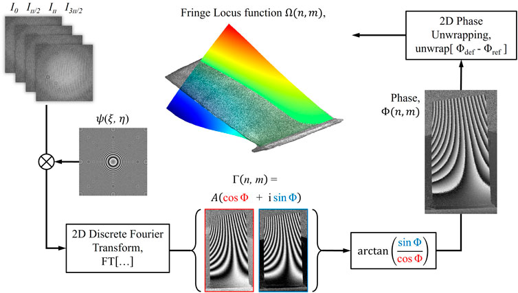
Figure 1. Schematic of the numerical reconstruction process. The phase shifted holograms are recorded and then multiplied by a 2D chirp function,
The reconstructed complex field is denoted by
and
where
The reconstructed field is complex in nature,
where
2.1.2 Double exposure method
The optical phase calculated from a single reconstructed field would yield static information, and thus, changes to the optical phase are measured interferometrically via a double exposure (DE) method. In this method, a hologram of an “undeformed” reference state is recorded and subsequently subtracted from “deformed” states of the object. This operation yields the phase difference, which for simplification of algorithm, can be directly calculated by,
Due to the nature of the four-quadrant inverse tangent, the phase values are wrapped within
where
2.1.3 Numerical focusing
Conventional holographic methods, such as electro-speckle pattern interferometry (ESPI) and Stetson holographic interferometry, use imaging lenses which have a positive effective focal length to project the object plane onto the CCD plane (Kreis et al., 1997). Due to this, either the lenses or the CCD plane must be physically moved in order to modify the object plane’s distance. In lensless digital holography, as described in Section 2.1.1, the complex field is numerically reconstructed at the object plane, and therefore, multiple fields at different distances can be reconstructed instantaneously, as shown in Figure 2. This is especially useful in circumstances where, for example, the sample’s geometry extends beyond the system’s depth-of-field (DOF) at the object plane, or there are multiple components at various distances to be inspected for comparative metrology purposes.
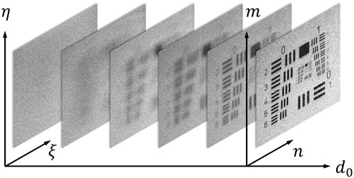
Figure 2. Instantaneous numerical focusing capabilities of lensless holography from a single phase-shifted hologram based on Fresnel approximation method. The complex field at the CCD plane
2.1.4 Reconstructed imaging parameters
The chirp function,
2.1.4.1 Field-of-view (FOV)
The field-of-view (FOV) of the reconstructed field is determined by the maximum angle permissible between the object and reference wavefronts. Therefore, the FOV is dependent on the geometrical constraints of the incoming reference as well as the CCD sensor. To satisfy the Nyquist criteria, the maximum accepted angle,
2.1.4.2 Resolution
The resolution of the reconstructed field can be determined by discretizing the FOV,
2.1.5 Enhancement of FOV by creation of virtual object
As mentioned in Section 1, an important in-situ and industrial metrology capability is the measurement of large FOV components. To fit such components within the maximum permissible angle of the object wavefront, described in Section 2.1.4.1, the working distance would need to be increased. This solution, however, will decrease the signal-to-noise ratio (SNR) and further expose the stability of the system to random external environmental fluctuations.
Therefore, in the measurement of components that do not fit within the reconstructed FOV, a negative lens is placed in front of the CCD. The negative focal length modifies the object wave incident ray angles, and therefore, larger angles now fit within the permissible range. Due to the inclusion of a lens, the reconstruction distance is modified, as shown in Figure 3. Mathematically, a virtual object, which is smaller than the real object and whose size depends on the focal length of the lens, is created at a distance,
where
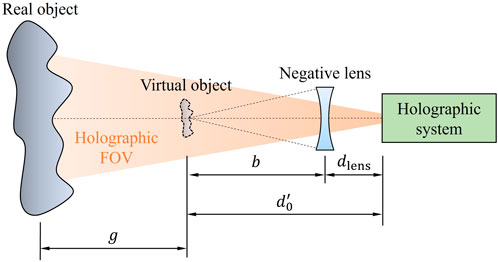
Figure 3. Creation of a virtual object for capturing large FOV samples by use of a negative focal length lens. Objects with areas which are outside of the holographic FOV, determined by the maximum permissible angle,
2.2 Stroboscopic modality
The measurement of high-speed motions typically requires high-speed recording devices. High-speed holographic interferometry has some advantages for industrial applications because the motions are captured within 5–20 ms (Ruiz-Cadalso and Furlong, 2023a; Ruiz-Cadalso and Furlong, 2023b), and thus, its sensitivity to external environmental disturbances is minimized. However, while the motions are repeatable, such as in the measurement of vibration deformations, a conventional CCD camera can be used as long as the illumination is strobed at the same frequency of the repeating high-speed motions. Therefore, for measurement of vibrations and acoustics, both the object and reference beams are strobed using an acousto-optic modulator (AOM). In these applications, the object motions are induced by sinusoidal excitations either mechanically or acoustically. In order to successfully strobe the illumination, the AOM is placed in front of the laser, interacting with the original beam prior to being split into reference and object counterparts. As part of the opto-electronic holographic system, a dual-channel arbitrary function generator (AFG) is used. The first channel generates the sinusoidal excitation signal which is used to stimulate the object, and the second channel generates a pulsed signal used for strobing. The pulse signal serves as a TTL interface for the AOM in order to engage it at the high-level range and disengage it at the low-level range. The frequencies of both channels are locked at the same value in order to avoid a frequency drift.
The AOM may be used as long as the response time is within 2.5% of the period of the high-speed motion. The pulse width, often called the duty cycle, of the strobe signal determines the percentage of the vibration cycle that is being illuminated, and it is typically 2%–5% (Flores Moreno et al., 2011; Khaleghi et al., 2013). The optimized duty cycle will depend on the frequency of excitation and the instantaneous velocity (temporal slope of deformation) of the motion that is being measured. With this configuration, specific instances of the vibration cycle can be captured by controlling the phase of the strobe signal as long as the excitation signal is phase-locked. The measurement procedure consists of first capturing a reference “undeformed” state of the object when the strobe phase is at
2.3 Design of experimental setup
The design of the opto-electronic holographic setup is displayed in Figure 4. The setup consists of a mechanical positioner, shown in Figure 4A, an optical head (OH), shown in Figures 4A, B laser delivery (LD) and the computer, instrumentation and software (CIS), shown in Figure 4C. A continuous-wave single-longitudinal-mode laser (Coherent, Inc. 315M-50 SL) generates a 50 mW beam with a diameter of 1 mm and a center wavelength of 532 nm in the LD in free-space and is subsequently diffracted by a Tellurium dioxide (TeO2) AOM (G&H Photonics 23110-1-LTD) with a rise time of 159 ns. The first order diffraction, which is modulable by the AOM as described in Section 2.2, is divided into two using a 10:90 beam splitter, reflecting 10% (reference beam) and transmitting 90% (object beam). Two externally triggered optical beam shutters are placed subsequent to the beam splitter, one on each path, in order to compute the beam ratio for optimization of fringe contrast. The reference beam is then deviated 90° by a mirror mounted onto a piezo-electric transducer (PZT) used for phase shifting. Both object and reference beams are then coupled into singlemode optical fibers 2.5 m in length using five-axis fiber-optic positioners (Newport 9131NF). At the OH, the optical fibers are connected to custom-manufactured opto-mechanics. The object beam fiber-optic output is expanded using a bi-concave lens prior to being illuminated onto the sample of interest. The reference beam is deviated 90° by a mirror and subsequently interfered with the scattered object irradiance via a 50:50 beam combiner. The superposition of the wavefronts is captured and recorded by a 5 MP (2,456
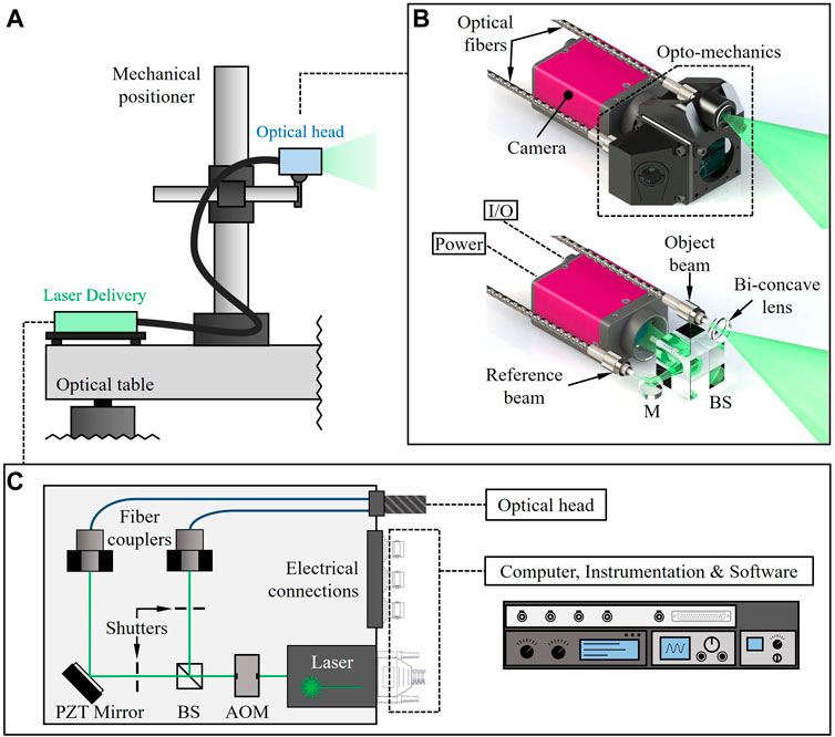
Figure 4. Designed opto-electronic setup for lensless stroboscopic digital holographic measurements: (A) integration of subsystems depicting the laser delivery (LD) connected to the optical head (OH) which is attached to the mechanical positioner; (B) the opto-mechanical design of the OH; and (C) the LD components and its connections to the OH and computer, instrumentation and software (CIS). I/O is trigger input/output, M is mirror, and BS is beam splitter.
2.3.1 Sensitivity vector variations
The stability of holographic systems relies, among other factors, on minimizing the absolute displacements, which are typically induced by external environmental disturbances, between the OH and the sample of interest along the sensitive direction. To correctly tackle the stability problem in digital holography, the sensitivity direction must be determined. This parameter depends on the sensitivity vector of the system, which is derived by the opto-geometric constraints between the OH setup and a sample of interest.
A schematic depicting the geometric constraints of the optical rays as well as their respective modifications during deformation of the sample is shown in Figure 5. The illumination of a point,
where
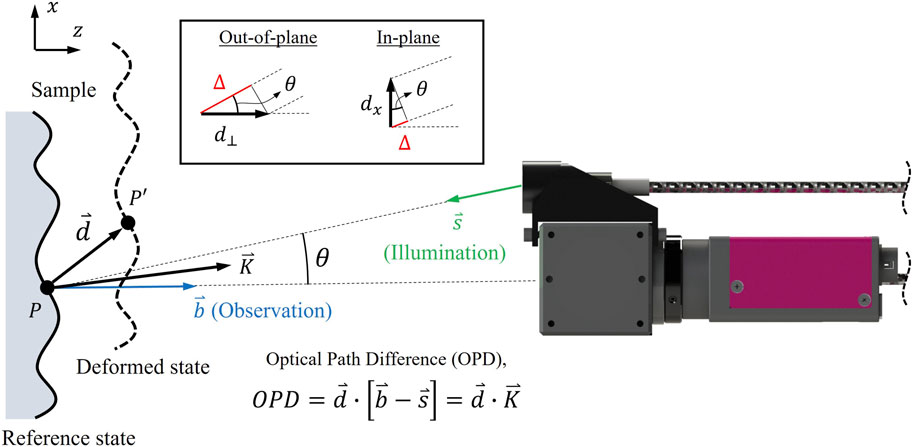
Figure 5. Schematic of geometrical arrangement for determination of sensitivity. When a sample undergoes a local displacement,
2.3.2 Stability
As discussed in the previous section, the stability of a holographic system is determined by its robustness to external factors which disturb the OPD between the reference and object beams. These disturbances can be categorized as either short- (transient) or long-term (steady-state). The stability of the system must be validated for these conditions in order to determine which applications it is suitable for.
The short-term stability of the system is studied by analyzing the mean optical phase,
where
3 Implementation and validation
3.1 Realized opto-electronic holographic setup
The realized opto-electronic setup for lensless digital holography is depicted in Figure 6. The LD subsystem is enclosed, and the optical fibers for reference and object beams connecting to the OH are encased in a stainless-steel jacket. The OH setup is attached to the end-effector of a custom-built mechanical positioner (Dobrev et al., 2010). The positioner’s base can be screwed onto the optical table for fixturing and disengaged for free positioning along the X-Z plane. The tower component contains two rack-and-pinion mechanisms, one for Y-adjustments (height) and the other for Z-adjustments. For additional degrees of freedom, a gimbal mount was installed for
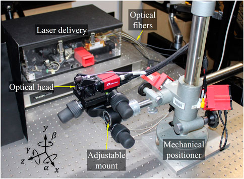
Figure 6. Realized opto-electronic holographic setup. The LD subsystem is enclosed, and the reference and object beam fibers which connect to the OH are encased in a stainless-steel jacket for protection. The OH is attached to the end-effector of the mechanical positioner, which has 7 degrees of freedom for high dexterity.
3.2 Validation of measuring performance
Various capabilities of the lensless holographic system are characterized as needed for in-situ metrology. The measurement and imaging performances are validated with the use of standardized samples. Throughout this section, the imaging resolution, DOF, and temporal stability are fully characterized prior to determining the system’s use for particular applications.
3.2.1 Imaging resolution
The spatial resolution of the system is validated with the use of a standardized resolution test target (USAF 1951). The target is positive, using a chrome pattern with clear background, and a white glass is placed behind to use as a background for improvement of contrast. The specific target has no birefringence and is therefore not polarization dependent. It can be used to characterize spatial resolutions from 1 to 57 lp/mm (Groups 0–5). The system is tested for working distances (WD’s) of 200, 500 and 1,000 mm. In order to achieve high uniformity in illumination distribution at each WD, the top-hat diffuser, described in Section 2.3, was used. The results are depicted in Figure 7, where Figure 7A shows the intensities of the reconstructed fields at each WD, and Figure 7B contains a plot comparing the cross-sectional distribution profiles of each field. The reconstructed intensities show groups 0 and 1, and zoomed-in versions show groups 2 and 3. The plot shows the intensity profiles for elements 1 through 6 in groups 0, 1 and 2 for all three WD’s. The validated resolutions determined are approximately 12.7, 9, and 5 lp/mm for WD’s 200, 500 and 1,000 mm, respectively.
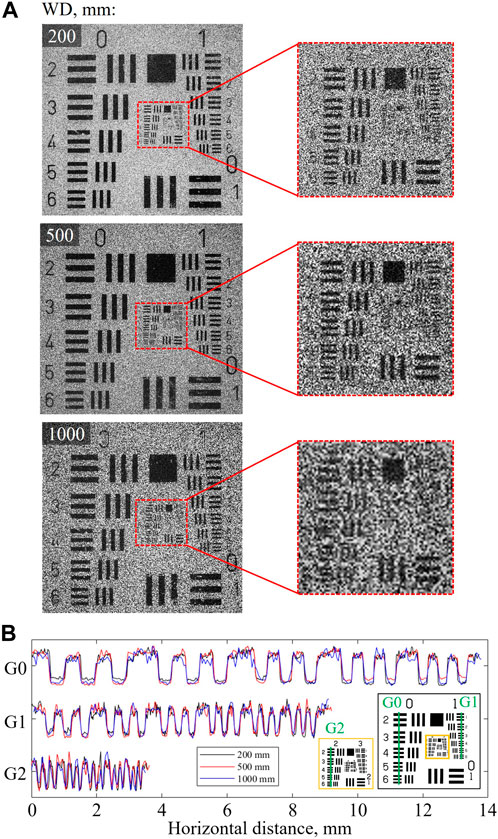
Figure 7. Validation of spatial resolution using a standard USAF resolution test target for three working distances (WD): (A) field intensity reconstructions of the target; and (B) cross-sectional intensity profiles of groups 0 (G0), 1 (G1), and 2 (G2). Zoomed-in cut-out sections are included for visualization of G2 in each WD. The determined resolutions for each WD are approximately 12.7, 9 and 5 lp/mm for 200, 500 and 1,000 mm, respectively.
3.2.2 DOF
The DOF of the system is characterized using a contrast target designed with one row of line pairs at 5 lp/mm. The line pairs are imaged perpendicularly with respect to the optical axis of the OH. Similar to the validations of spatial resolution, the system’s DOF is tested for WD’s of 200, 500 and 1,000 mm. At each WD, the OH is displaced over an array of stepped positions relative to the focal plane in order to measure the variability of defocusing. The results are depicted in Figure 8, where Figure 8A shows the intensities of the reconstructed fields at three chosen OH positions for each WD, Figure 8B depicts a plot of the intensity profiles of each field, and Figure 8C depicts the degree of defocusing trend calculated for each WD. The degree of focus is quantified by a Gaussian derivative filter and curve fitted with a Gaussian function. The DOF, which is twice that of the half-width at half-maximum (HWHM), is computed for each WD to be approximately 10, 50 and 360 mm for 200, 500 and 1,000 mm, respectively.
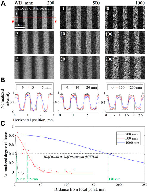
Figure 8. Validation of reconstructed depth-of-field (DOF) using a contrast target at each WD: (A) field intensity reconstructions at three OH positions; (B) 1D intensity profile plots of the line pairs; and (C) a plot of the quantified degree of focus. The legend in (B) delineates the OH distances from the focal plane. The degree of focus is quantified for each position from the focal plane by a Gaussian derivative filter, and the results are curve fitted by a Gaussian function. The determined DOF’s for each WD are approximately 10, 50 and 360 mm for 200, 500 and 1,000 mm, respectively.
3.2.3 Temporal stability
As discussed in Section 2.3.2, both transient and steady-state disturbances are characterized for validation of stability. The testing target is chosen to be a mechanically rigid artificial sample with negligible time-varying behaviors. Considering the variety of positioning requirements for in-situ metrology, the stability of the system will be validated for two setup configurations, first with a pitch angle of 0° (forward), and second with a pitch angle of 90° (top-down). Given the structural design of the mechanical positioner, the external disturbances have a varying effect on the stability of the system depending on the measurement orientation. For simplicity, throughout this section, the first setup configuration will be referred to as forward optical head (FOH), and the second as downward optical head (DOH). The results are shown in Figure 9, where Figures 9A, B display the FOH and DOH configurations, respectively.
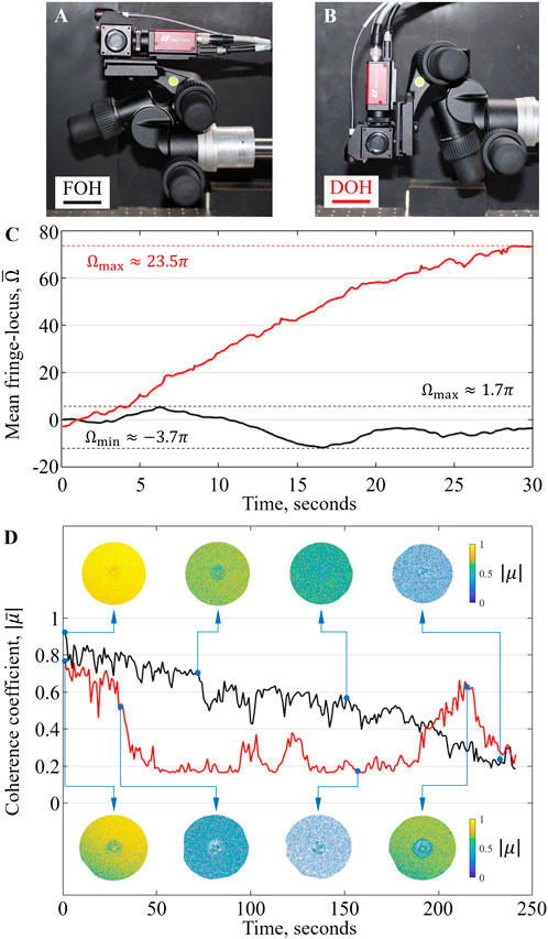
Figure 9. Validation of temporal stability: (A) first configuration studied named forward optical head (FOH); (B) second configuration studied named downward optical head (DOH); (C) short-term validation by mean optical phase throughout a 30s recording; (D) long-term validation by time lapse characterization of speckle decorrelation with a plot of the mean
Short-term stability validations are shown in Figure 9C. This set of measurement considers mainly transient disturbances and is done by computing the mean optical phase distribution in a recorded video. The video is approximately 30 s long and contains 300 frames of the extracted optical phase. As seen from the plot, the FOH configuration proves more stable than DOH since it deviates between
Long-term stability validations are shown in Figure 9D. This set of measurement considers mainly steady-state disturbances and is done by studying the decorrelation of speckles in DE holograms, as described in Section 2.3.2, as long as the reference hologram is unchanged for the complete measurement dataset. The degree of speckle decorrelation is computed by solving for the magnitude of the modulus of complex coherence coefficient during a time lapse measurement that lasts 4 h. As seen from the plot, the mean coherence factor computed for FOH is linearly decreasing at a slope of approximately
4 Representative results
4.1 Vibration measurements in aerospace turbomachinery components
Understanding the frequency response of a dynamic system is critical in the aerospace industry for characterizing the performance and behavior of turbomachinery components. The information that is recovered is crucial for predicting a component’s response to particular dynamic loads such as high-pressure rapid currents of air and random turbulence. Optical techniques such as Digital Image Correlation (DIC), Electro-Speckle Pattern Interferometry (ESPI) and Stetson holographic interferometry have been thoroughly exploited for use in the aerospace industry (Stetson, 1978; Pryputniewicz and Stetson, 1990; Stetson and Weaver, 2011).
4.1.1 Turbine blades with complex geometries
A particular interest in the field is the measurement of leading and trailing edges of a turbine blade. For such blades with complex geometries, it is challenging for most conventional techniques given the variability of measurement sensitivity that arises from a highly diversified surface normal vector. A solution previously used is the placement of a mirror to inspect both edges with maximized sensitivity in each. In DIC and ESPI methods, if the DOF is not high enough to cover both projections, at least two exposures must be taken for each edge due to their dependance on the projection of the object plane onto the sensor plane via a positive lens configuration. In lensless digital holography, the numerical focusing capabilities allow for the instantaneous reconstruction of fields at the leading and trailing edges.
4.1.1.1 Setup configuration for sensitivity optimization
With the placement of a mirror, lensless digital holography can be used to instantaneously reconstruct the fields at leading and trailing edges of a turbine blade with complex geometry. The experimental configuration can be seen in Figure 10, with a schematic visually describing the optimization of the sensitivity vector in Figure 10A, and the experimental configuration in Figure 10B. The sample is a titanium alloy aerospace compressor blade with approximate dimensions of 40
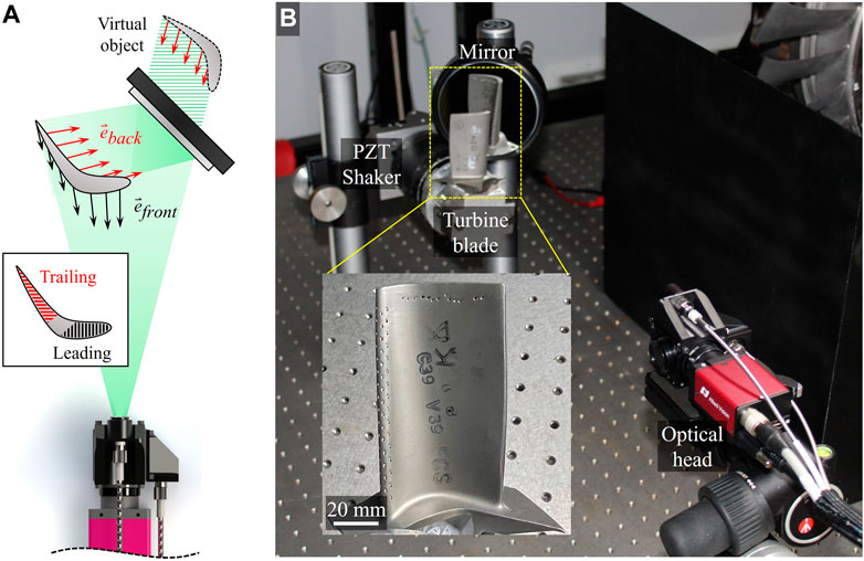
Figure 10. Configuration of OH setup and alignment for sensitivity optimization in leading and trailing edges: (A) schematic of setup depicting the geometrical configuration for maximizing sensitivity vectors in each edge; and (B) realized configuration with real turbine blade sample. The mirror is placed at a particular location and orientation such that a virtual object of the back of the turbine blade is created within the system’s FOV and the sensitivity is maximized at the trailing edge.
4.1.1.2 Instantaneous measurements of leading and trailing edges
The results for instantaneous vibration measurements of leading and trailing edges of turbine blades with complex geometries are displayed in Figure 11. Time averaged holograms as well as vibration deformations are shown for excitation frequencies of 2.49, 4.16, and 8.84 kHz in Figures 11A, B, and Figure 11C, respectively. For each frequency, the time averaged holograms are shown for the reconstructed fields at the leading and trailing edges in the first two columns. The third column displays the quantified deformation plot from the DE holograms. It can be seen when comparing the data between unoptimized and optimized regions of the trailing edge that the alignment of the surface normal vectors with respect to the sensitivity vectors of the holographic system is crucial to obtaining high quality results with low SNR.
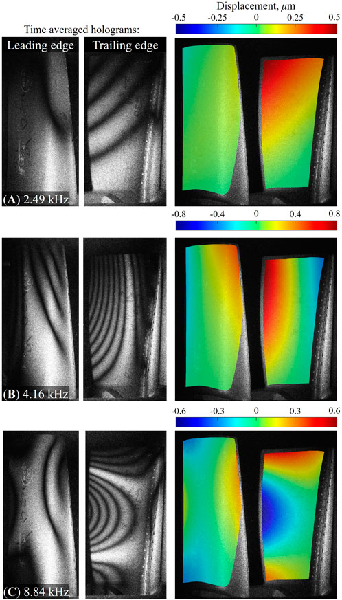
Figure 11. Instantaneous vibration measurements of leading and trailing edges for three frequencies: (A) 2.49 kHz; (B) 4.16 kHz; and (C) 8.84 kHz. For each frequency, the time averaged holograms of the leading and trailing edges are shown, as well as the strobed vibration deformations quantified. As seen, the matching of the direction of sensitivity vectors to the surface normal is crucial for obtaining high quality results with low SNR.
4.1.2 Complete mode shape analysis of large aerospace rotors
The individual blade that was tested with in the previous section is one of multiple that form part of a turbomachinery component called a rotor. In the aerospace industry, aside from characterizing the individual mode shapes of each blade, the measurement of a complete rotor is of high interest. Characterizing the mode shape of a rotor provides an understanding of the dynamic behavior of the entire assembly and is especially important in the avoidance of superimposed resonance in which every individual blade resonates with the same loading frequency.
4.1.2.1 Stitched time averaged holograms of rotor mode shapes
The sample used is a testing rotor for which the source, model, and measured data such as loading frequency and displacement data, among other parameters, are omitted due to nondisclosure agreements. The sample was loaded with the use of a PZT shaker attached to a particular location around the rim. The mode shapes for two frequencies were acquired for the complete rotor by recording multiple holograms which are subsequently laterally stitched to cover for the large size of the rotor. Each measurement is taken using the same frequency, and the OH is moved with the use of the mechanical positioner. The results are shown in Figure 12. Figure 12A displays the experimental setup depicting the OH and the rotor component. A reconstructed intensity image of the entire rotor blade is shown in Figure 12B. In order to enhance the FOV as necessary, a compound lens configuration with an effective focal length of −13.6 mm was used, as described in Section 2.3, and the illumination angle and uniformity was provided by a 50° top-hat diffuser. However, due to limited spatial frequency from the CCD sensor, the short fringe spacing is not able to be captured with the enhanced FOV. Therefore, individual blade mode shapes are measured and stitched together. The stitched representative measurements of the rotor’s mode shape are shown in Figures 12C, D.
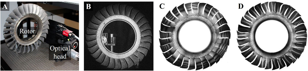
Figure 12. Vibration measurements of large rotor blade: (A) experimental setup showing the OH and the rotor; (B) reconstructed intensity with enhanced FOV; (C) stitched time averaged hologram for one frequency; and (D) stitched time averaged holograms for second frequency. The enhancement of FOV for (B) was provided by a compound lens assembly with an effective focal length of −13.6 mm. Stitched measurements were conducted due to low spatial resolution with the enhanced FOV. Frequency data as well as quantifications are not shown due to nondisclosure agreements.
4.2 Transient thermo-mechanical deformations in heat sinks
Heat sinks are crucial components to thermal management systems and are vital to various industrial applications, particularly in electronics and manufacturing. The thermo-mechanical deformations that these components endure are a direct consequence of the interactions between thermal effects and mechanical forces within the heat sink’s fins, leading to alterations in their structural integrity and performance. A specific area of interest is gaining a comprehensive understanding of the deformations occurring within the fin structures themselves. Therefore, characterizing these deformations and their impact on the overall performance of the heat sink is vital for optimizing thermal management strategies and ensuring the efficient operation of electronic components.
4.2.1 Experimental configuration
The sample used for this experiment is an aluminum heat sink designed for packaged electronics. The experimental configuration is shown in Figure 13, along with intensity reconstructions focused on different planes throughout the length of the heat sink fin. In the setup, as depicted in Figure 13A, the OH is aligned with respect to the heat sink sample, which is attached via a thermal paste onto a thermo-electric heater (TEH). The TEH is externally controlled from software and has a temperature stabilization range of 0.1°C. An infrared (IR) camera is used to inspect the temperature distribution throughout the length of the heat sink, and thus, is placed in perpendicular fashion. Figures 13B, C, and Figure 13D show the reconstructed intensities of the heat sink from a single phase-shifted hologram numerically focused on the front-plane, mid-plane, and back-plane of the heat sink, respectively.
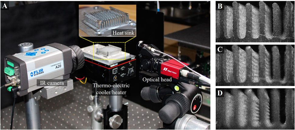
Figure 13. Setup for lensless holographic reconstructions of the interior of a heat sink: (A) experimental configuration with OH, heat sink, IR camera, and thermo-electric heater (TEH); and reconstructed intensities of the heat sink fin numerically focused on the (B) front-plane; (C) mid-plane; and (D) back-plane. The TEH is externally controlled through software and is used to increase the temperature in the heat sink. The IR camera is used to monitor the temperature distribution throughout the measurements.
4.2.2 Interior thermal expansions in a heat sink fin
Transient thermal deformations are measured throughout the interior surface of a heat sink fin, as shown in Figure 14. The experimental procedure consists of thermally loading the heat sink by increasing the top surface temperature of the TEH, where the sample’s bottom surface is thermal pasted, from 25 to 27°C. Throughout the temperature increase, a video of the optical phase is recorded at approximately 10 fps. A selected number of frames throughout the measurement are shown in Figure 14A, alongside the temperature field quantified by the IR camera. The DE holograms are divided into multiple sections at different distances along the heat sink fin and are each individually numerically reconstructed and unwrapped to compute the fringe-locus function,
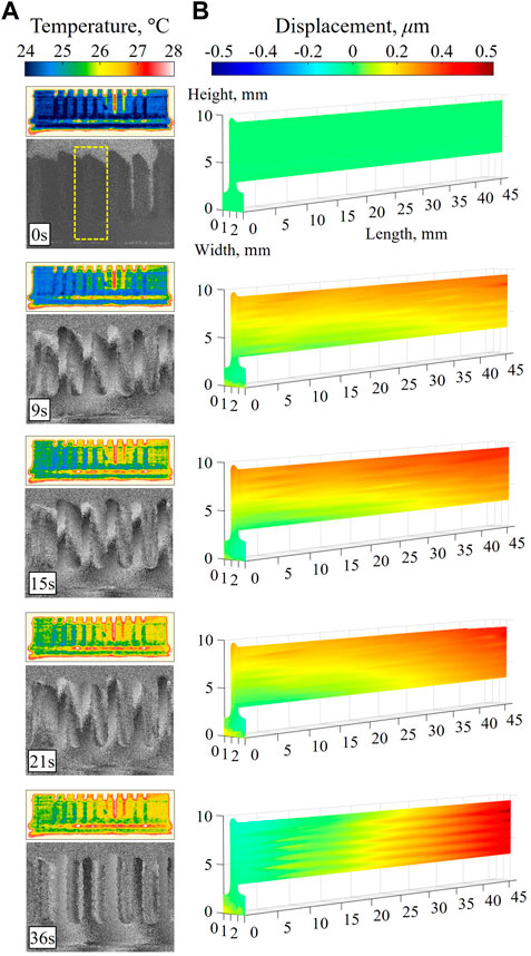
Figure 14. Thermo-mechanical deformations of heat sink shown for timestamps 0s, 9s, 15s, 21s, and 36s: (A) optical phase from DE holograms along with temperature fields from IR camera; and (B) deformation measurements stitched from individually reconstructed fields at various distances from the front to the back of the heat sink. Due to short-term instabilities and disturbances, the deformations are measured relative to the front-plane, and thus, are not regarded as absolute.
4.3 Acoustic deformations for the study of hearing mechanics
Acoustics play a fundamental role in the field of hearing mechanics, where the intricate interaction between sound waves and the human auditory system is extensively studied. Understanding the acoustically induced deformations within the human ear is pivotal for advancing comprehension of hearing mechanisms and the diagnosis of auditory disorders.
The pinna plays a crucial role in the initial stages of sound capture and localization within the hearing process and has a direct relationship with the frequency response of the auditory system. Therefore, characterizing the acoustical response leads to further understanding the performance of the ear in areas such as directionality detection and speech perception, as well as contributing to the design of hearing assistive devices. Additionally, measuring the acoustical response of both the front (anterior) and back (posterior) of the ear is of interest and has practical applications, for example, in hearing device design, binaural hearing research, and audiological assessments, contributing to our understanding of how the ear processes sound in various listening scenarios.
4.3.1 Instantaneous anterior and posterior measurements of a synthetic pinna
The test sample is a synthetic left pinna with anthropometric concha and ear canal made of soft silicone material. The sample was designed and fabricated to resemble the human pinna both in structure and performance to aid in the development of supra-aural and circum-aural earphones. Therefore, the frequency response and acoustic characteristics of this sample closely mimic that of a real human pinna. The results are shown in Figure 15. Figure 15A shows the experimental configuration used for these measurements as well as results. An acoustic speaker with a frequency range of 0–20 kHz is placed on the top surface of the optical table and below the sample. A mirror is placed behind the sample at a particular position and orientation such that the posterior of the ear is projected within the FOV of the holographic system.
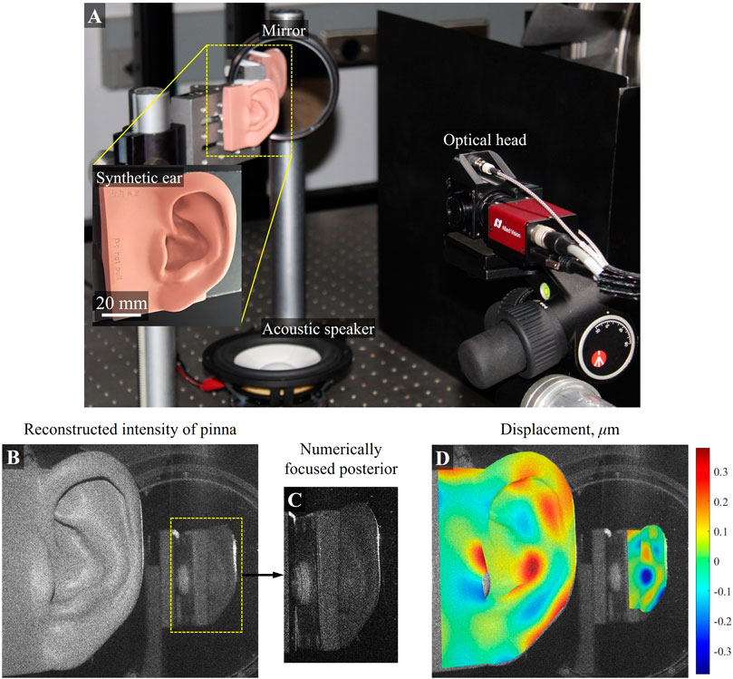
Figure 15. Acoustically induced vibration deformations in a synthetic pinna: (A) experimental configuration depicting the OH, the pinna, an acoustic speaker as the loading mechanism, and the mirror for posterior measurements; (B) reconstructed intensity of the pinna numerically focused on the anterior; (C) reconstructed intensity numerically focused on the posterior; and (D) quantified vibration deformation of both sides of the pinna overlayed on the intensity image. The pinna was acoustically loaded at 350 Hz.
Acoustically induced deformations on the synthetic pinna are measured in full-FOV. The reconstructed intensity of the anterior of the sample is shown in Figure 15B, and that of the posterior is shown in Figure 15C. The sample was stimulated with the use of the acoustic speaker at 350 Hz, and the deformation field for both anterior and posterior sides are instantaneously measured, as shown in Figure 15D.
5 Discussions
The multifaceted capabilities of lensless DHI have been exploited over a broad spectrum of measurement and loading conditions, both transient and steady-state. The instantaneous reconstruction of a field at any given distance has been applied to a variety of applications, from aerospace to thermo-mechanics, and hearing mechanics. In aerospace, the instantaneous vibration measurements of turbine blade leading and trailing edges were demonstrated by optimization of the sensitivity vectors using a mirror. Additionally, time averaged holograms are shown for large FOV turbomachinery rotors. The fins of heat sinks are often long parts which individually undergo thermo-mechanical deformations, and with the use of lensless DHI, various fields throughout a single fin were reconstructed and stitched together to study the effects of thermal loads. Lastly, acoustically induced vibrations of anterior and posterior areas of a synthetic pinna with anthropometric concha and ear canal are instantaneously quantified.
The results presented in this paper serve as a representative demonstration of in-situ metrological capabilities of lensless DHI given specific measurement and loading conditions over various applications. Nevertheless, it is important to note that some discussed metrological challenges were not formally addressed in the applied measurements. These measurements were conducted under controlled environmental conditions that, while suitable for this investigation, may not fully reflect the stringent stability requirements typically demanded by in-situ and industrial metrology. Furthermore, the large rotor blade measurements were constructed from stitched time averaged holograms of each individual blade. This approach was necessitated by the spatial resolution limitations of the CCD sensor, which, due to the enhanced FOV, could not sufficiently capture the short fringe spacing for every blade separately. The transient thermo-mechanical deformation measurements were especially challenging due to large absolute deformations that introduced a high degree of speckle decorrelation. Despite the aforementioned discussion points, this paper underscores the potential of lensless DHI in industrial applications while also acknowledging the need for further research and advancements.
Related work in this area is continually exploiting the capabilities of new and advanced holographic methods. As mentioned previously, temporal instability is a significant challenge for DHI within industrial settings, and this could be overcome with innovative phase retrieval methods such as single-shot dual-wavelength (Wang et al., 2016), space-time paradigm (Wang et al., 2023), parallel phase shifting (Du et al., 2023), optical vortex phase shifting (Qiu et al., 2023), and deep neural networks (Aleksandrovych et al., 2023), among others. Furthermore, the ability to instantaneously reconstruct the optical field at any given distance can be automated with advanced algorithms (Memmolo et al., 2011). At the reconstructed image, the DOF is a vital parameter in acquiring high-quality phase data in complex-shaped objects, and techniques are being investigated to further enhance it (Ferraro et al., 2005). Different areas within recording and processing of digital holographic information need to be explored to further enhance its metrological capacity as applied to a wide range of industrial sectors.
Capabilities that are vital for in-situ and industrial metrology have been demonstrated with lensless DHI. The complex metrological challenges have been systematically addressed and the representative results from this paper showcase the unique attributes of this technology as applied to in-situ NDT, real-time imaging, and industrial quality control. As lensless DHI continues to evolve and innovative methodologies are developed, it emerges as a formidable contender capable of meeting particular demands of industrial applications.
Data availability statement
The datasets presented in Section 4.1.2 of this article are not readily available due to third party confidential disclosure agreements. All remaining data which supports the conclusions of this article will be made available by the authors, without undue reservation.
Author contributions
DR-C: Conceptualization, Data curation, Formal Analysis, Investigation, Methodology, Validation, Visualization, Writing–original draft, Writing–review and editing. CF: Resources, Supervision, Writing–review and editing, Conceptualization.
Funding
The author(s) declare that no financial support was received for the research, authorship, and/or publication of this article.
Conflict of interest
The authors declare that the research was conducted in the absence of any commercial or financial relationships that could be construed as a potential conflict of interest.
Publisher’s note
All claims expressed in this article are solely those of the authors and do not necessarily represent those of their affiliated organizations, or those of the publisher, the editors and the reviewers. Any product that may be evaluated in this article, or claim that may be made by its manufacturer, is not guaranteed or endorsed by the publisher.
References
Aleksandrovych, M., Strassberg, M., Melamed, J., and Xu, M. (2023). Polarization differential interference contrast microscopy with physics-inspired plug-and-play denoiser for single-shot high-performance quantitative phase imaging. Biomed. Opt. Express 14 (11), 5833–5850. doi:10.1364/boe.499316
Castellini, P., Martarelli, M., and Tomasini, E. P. (2006). Laser Doppler Vibrometry: development of advanced solutions answering to technology's needs. Mech. Syst. Signal Process. 20 (6), 1265–1285. doi:10.1016/j.ymssp.2005.11.015
Cubreli, G., Psota, P., Dančová, P., Lédl, V., and Vít, T. (2021). Digital holographic interferometry for the measurement of symmetrical temperature fields in liquids. Photonics 8 (6), 200. doi:10.3390/photonics8060200
De la Torre Ibarra, M. H., Flores Moreno, J. M., Aguayo, D. D., Hernández-Montes, M. D. S., Pérez-López, C., and Mendoza-Santoyo, F. (2014). Displacement measurements over a square meter area using digital holographic interferometry. Opt. Eng. 53 (9), 092009. doi:10.1117/1.oe.53.9.092009
Dobrev, I., Moreno, J. F., Furlong, C., Harrington, E. J., Rosowski, J. J., and Scarpino, C. (2010). Design of a positioning system for a holographic otoscope. SPIE Interferom. XV Appl. 7791, 109–120.
Du, Y., Li, J., Zhao, H., Zhao, Z., Fan, C., Zhou, M., et al. (2023). Accurate dynamic 3D deformation measurement based on the synchronous multiplexing of polarization and speckle metrology. Opt. Lett. 48 (9), 2329. doi:10.1364/ol.485969
Ebrahimi, S., Dashtdar, M., Anand, A., and Javidi, B. (2020). Common-path lensless digital holographic microscope employing a Fresnel biprism. Opt. Lasers Eng. 128, 106014. doi:10.1016/j.optlaseng.2020.106014
Ferraro, P., Grilli, S., Alfieri, D., De Nicola, S., Finizio, A., Pierattini, G., et al. (2005). Extended focused image in microscopy by digital holography. Opt. Express 13 (18), 6738–6749. doi:10.1364/opex.13.006738
Flores Moreno, J. M., Furlong, C., Rosowski, J. J., Harrington, E., Cheng, J. T., Scarpino, C., et al. (2011). Holographic otoscope for nanodisplacement measurements of surfaces under dynamic excitation. Scanning 33 (5), 342–352. doi:10.1002/sca.20283
Fu, Y., Shang, Y., Hu, W., Li, B., and Yu, Q. (2021). Non-contact optical dynamic measurements at different ranges: a review. Acta Mech. Sin. 37 (4), 537–553. doi:10.1007/s10409-021-01102-1
Ganesan, A. R., “Holographic and laser speckle methods in non-destructive testing,” Proceedings of the National Seminar and Exhibition on Non-Destructive Evaluation, Chennai, India, 126, 2009.
Hai, N., and Rosen, J. (2021). Single-plane and multiplane quantitative phase imaging by self-reference on-axis holography with a phase-shifting method. Opt. Express 29 (15), 24210–24225. doi:10.1364/oe.431529
Harding, K. (2008). Challenges and opportunities for 3D optical metrology: what is needed today from an industry perspective. France, Europe: SPIE Two- and Three-Dimensional Methods for Inspection and Metrology VI, 112–119.
Harrington, E., Dobrev, I., Bapat, N., Flores, J. M., Furlong, C., Rosowski, J., et al. (2010). Development of an optoelectronic holographic platform for otolaryngology applications. SPIE Interferom. XV Appl. 7791, 163–176.
Hernández-Montes, M. del S., Mendoza-Santoyo, F., Moreno, M. F., de la Torre-Ibarra, M., Acosta, L. S., and Palacios-Ortega, N. (2020). Macro to nano specimen measurements using photons and electrons with digital holographic interferometry: a review. J. Eur. Opt. Soc. Rapid Publ. 16 (1), 16. doi:10.1186/s41476-020-00133-8
Javidi, B., Carnicer, A., Anand, A., Barbastathis, G., Chen, W., Ferraro, P., et al. (2021). Roadmap on digital holography [Invited]. Opt. Express 29 (22), 35078–35118. doi:10.1364/oe.435915
Kakue, T., Yonesaka, R., Tahara, T., Awatsuji, Y., Nishio, K., Ura, S., et al. (2011). High-speed phase imaging by parallel phase-shifting digital holography. Opt. Lett. 36 (21), 4131. doi:10.1364/ol.36.004131
Khaleghi, M., Furlong, C., Ravicz, M., Cheng, J. T., and Rosowski, J. J. (2015a). Three-dimensional vibrometry of the human eardrum with stroboscopic lensless digital holography. J. Biomed. Opt. 20 (5), 051028. doi:10.1117/1.jbo.20.5.051028
Khaleghi, M., Guignard, J., Furlong, C., and Rosowski, J. J. (2015b). Simultaneous full-field 3-D vibrometry of the human eardrum using spatial-bandwidth multiplexed holography. J. Biomed. Opt. 20 (11), 111202. doi:10.1117/1.jbo.20.11.111202
Khaleghi, M., Lu, W., Dobrev, I., Cheng, J. T., Furlong, C., and Rosowski, J. J. (2013). Digital holographic measurements of shape and three-dimensional sound-induced displacements of tympanic membrane. Opt. Eng. 52 (10), 101916. doi:10.1117/1.oe.52.10.101916
Kozma, A., and Christensen, C. R. (1976). Effects of speckle on resolution. JOSA 66 (11), 1257–1260. doi:10.1364/josa.66.001257
Kreis, T. (2002). Frequency analysis of digital holography. Opt. Eng. 41 (4), 771–778. doi:10.1117/1.1458551
Kreis, T., Adams, M., and Jueptner, W. P. O. (1997). Methods of digital holography: a comparison. SPIE Opt. Insp. Micromeasurements II 3098, 224–233. doi:10.1117/12.281164
Kumar, M., Matoba, O., Quan, X., Rajput, S. K., Awatsuji, Y., and Tamada, Y. (2021). Single-shot common-path off-axis digital holography: applications in bioimaging and optical metrology [Invited]. Appl. Opt. 60 (4), A195. doi:10.1364/ao.404208
Kumar, M., Pensia, L., and Kumar, R. (2023). Highly stable vibration measurements by common-path off-axis digital holography. Opt. Lasers Eng. 163, 107452. doi:10.1016/j.optlaseng.2022.107452
Kumar, R., and Dwivedi, G. (2023). Emerging scientific and industrial applications of digital holography: an overview. Eng. Res. Express 5 (3), 032005. doi:10.1088/2631-8695/acf97e
Kumon, Y., Hashimoto, S., Inoue, T., Nishio, K., Kumar, M., Matoba, O., et al. (2023). Three-dimensional video imaging of dynamic temperature field of transparent objects recorded by a single-view parallel phase-shifting digital holography. Opt. Laser Technol. 167, 109808. doi:10.1016/j.optlastec.2023.109808
Lagny, L., Secail-Geraud, M., Le Meur, J., Montresor, S., Heggarty, K., Pezerat, C., et al. (2019). Visualization of travelling waves propagating in a plate equipped with 2D ABH using wide-field holographic vibrometry. J. Sound. Vib. 461, 114925. doi:10.1016/j.jsv.2019.114925
Memmolo, P., Distante, C., Paturzo, M., Finizio, A., Ferraro, P., and Javidi, B. (2011). Automatic focusing in digital holography and its application to stretched holograms. Opt. Lett. 36 (10), 1945–1947. doi:10.1364/ol.36.001945
Meteyer, E., Foucart, F., Pezerat, C., and Picart, P. (2021). Modeling of speckle decorrelation in digital Fresnel holographic interferometry. Opt. Express 29 (22), 36180–36200. doi:10.1364/oe.438346
Montresor, S., Tahon, M., Laurent, A., and Picart, P. (2020). Computational de-noising based on deep learning for phase data in digital holographic interferometry. Apl. Photonics 5 (3), 030802. doi:10.1063/1.5140645
Mustafi, S., and Latychevskaia, T. (2023). Fourier transform holography: a lensless imaging technique, its principles and applications. Photonics 10 (2), 153. doi:10.3390/photonics10020153
Newman, J. W. (2005). Holographic and shearographic NDT applications in aerospace manufacturing. Mater. Eval. 63 (7).
O'Donoughue, P., Gautier, F., Meteyer, E., Durand-Texte, T., Secail-Geraud, M., Foucart, F., et al. (2023). Comparison of three full-field optical measurement techniques applied to vibration analysis. Sci. Rep. 13 (1), 3261. doi:10.1038/s41598-023-30053-9
Picart, P. (2021). Recent advances in speckle decorrelation modeling and processing in digital holographic interferometry. Photonics Lett. Pol. 13 (4), 73. doi:10.4302/plp.v13i4.1126
Picart, P., Leval, J., Mounier, D., and Gougeon, S. (2005). Some opportunities for vibration analysis with time averaging in digital Fresnel holography. Appl. Opt. 44 (3), 337–343. doi:10.1364/ao.44.000337
Pryputniewicz, R. J. (1985). Time average holography in vibration analysis. Opt. Eng. 24 (5), 843–848. doi:10.1117/12.7973586
Pryputniewicz, R. J. (1988). Vibration studies using heterodyne hologram interferometry. SPIE Ind. Laser Interferom. II 955, 154–161. doi:10.1117/12.947681
Pryputniewicz, R. J., and Stetson, K. A. (1990). Measurement of vibration patterns using electro-optic holography. SPIE Laser Interferom. Quantitative Analysis Interf. Third a Ser. 1162, 456–467.
Psota, P., Çubreli, G., Šimurda, D., Šidlof, P., Kredba, J., Stašík, M., et al. (2023). Noise-resistant two-wavelength interferometry for single-shot measurement of high-gradient flows. Opt. Lasers Eng. 164, 107505. doi:10.1016/j.optlaseng.2023.107505
Qiu, H., Liu, X., Wang, K., Dou, J., Di, J., and Qin, Y. (2023). Real-time phase measurement of optical vortex via digital holography. Front. Phys. 11, 1190616–1192023. doi:10.3389/fphy.2023.1190616
Ruiz-Cadalso, D., and Furlong, C. (2023a). “Comparative study of high-speed digital holographic interferometry and scanning laser Doppler vibrometry for modal analysis,” in Proc., SEM 2023 Annu. Conf., Orlando, FL, USA.
Ruiz-Cadalso, D., and Furlong, C. (2023b). “Non-destructive crack detection by high-speed digital holographic interferometry and impact-induced travelling waves,” in Proc., SEM 2023 Annu. Conf., Orlando, FL, USA.
Schnars, U., Kreis, T. M., and Jueptner, W. P. O. (1996). Digital recording and numerical reconstruction of holograms: reduction of the spatial frequency spectrum. Opt. Eng. 35 (4), 977–982. doi:10.1117/1.600706
Stetson, K. A. (1978). The use of an image derotator in hologram interferometry and speckle photography of rotating objects. Exp. Mech. 18, 67–73. doi:10.1007/bf02324502
Stetson, K. A., and Weaver, G. (2011). A study of pseudo-free mounting of turbine blades for digital holographic vibration analysis and modal assurance criteria calculations. Exp. Tech. 35 (6), 80–85. doi:10.1111/j.1747-1567.2010.00679.x
Tahara, T., Takahashi, Y., Komura, T., Kaku, T., and Arai, Y. (2015). Single-shot multiwavelength digital holography using angular multiplexing and spatial bandwidth enhancement for extending the field of view. J. Disp. Technol. 11 (10), 807–813. doi:10.1109/jdt.2015.2424082
Wang, Z., Bianco, V., Maffettone, P. L., and Ferraro, P. (2023). Phase-retrieval in scanning digital holography for optofluidics. SPIE Opt. Methods Insp. Charact. Imaging Biomaterials VI 12622, 173–176.
Wang, Z., Jiang, Z., and Chen, Y. (2016). Single-shot dual-wavelength phase reconstruction in off-axis digital holography with polarization-multiplexing transmission. Appl. Opt. 55 (22), 6072–6078. doi:10.1364/ao.55.006072
Wang, Z., Miccio, L., Coppola, S., Bianco, V., Memmolo, P., Tkachenko, V., et al. (2022). Digital holography as metrology tool at micro-nanoscale for soft matter. Light Adv. Manuf. 3 (1), 151–176. doi:10.37188/lam.2022.010
Xia, P., Ri, S., Inoue, T., Awatsuji, Y., and Matoba, O. (2021). Dynamic phase measurement of a transparent object by parallel phase-shifting digital holography with dual polarization imaging cameras. Opt. Lasers Eng. 141, 106583. doi:10.1016/j.optlaseng.2021.106583
Xu, X., Luo, W., Wang, H., and Wang, X. (2023). Robust holographic reconstruction by deep learning with one frame. Photonics 10 (10), 1155. doi:10.3390/photonics10101155
Zhang, J., Dai, S., Ma, C., Xi, T., Di, J., and Zhao, J. (2021). A review of common-path off-axis digital holography: towards high stable optical instrument manufacturing. Light Adv. Manuf. 2 (3), 1. doi:10.37188/lam.2021.023
Keywords: digital holographic interferometry, in-situ, industrial applications, numerical focusing, non-destructive testing (NDT), real-time lensless imaging
Citation: Ruiz-Cadalso D and Furlong C (2024) High-resolution imaging for in-situ non-destructive testing by quantitative lensless digital holography. Front. Photonics 5:1351744. doi: 10.3389/fphot.2024.1351744
Received: 06 December 2023; Accepted: 21 March 2024;
Published: 13 May 2024.
Edited by:
Claas Falldorf, Bremer Institut für Angewandte Strahltechnik, GermanyReviewed by:
Sara Coppola, National Research Council (CNR), ItalyAdam Styk, Warsaw University of Technology, Poland
Copyright © 2024 Ruiz-Cadalso and Furlong. This is an open-access article distributed under the terms of the Creative Commons Attribution License (CC BY). The use, distribution or reproduction in other forums is permitted, provided the original author(s) and the copyright owner(s) are credited and that the original publication in this journal is cited, in accordance with accepted academic practice. No use, distribution or reproduction is permitted which does not comply with these terms.
*Correspondence: Daniel Ruiz-Cadalso, ZGFydWl6Y2FkYWxzb0B3cGkuZWR1