Influence of the Signal-To-Noise Ratio on Variance of Chromophore Concentration Quantification in Broadband Near-Infrared Spectroscopy

This study presented a theoretical or analytical approach to quantify how the signal-to-noise ratio (SNR) of a near infrared spectroscopy (NIRS) device influences the accuracy on calculated changes of oxy-hemoglobin (Δ[HbO]), deoxy-hemoglobin (Δ[HHb]), and oxidized cytochrome c oxidase (Δ[oxCCO]). In theory, all NIRS experimental measurements include variations due to thermal or electrical noise, drifts, and disturbance of the device. Since the computed concentration results are highly associated with device-driven variations, in this study, we applied the error propagation analysis to compute the variability or variance of Δ[HbO], Δ[HHb], and Δ[oxCCO] depending on the system SNR. The quantitative expressions of variance or standard deviations of changes in chromophore concentrations were derived based on the error propagation analysis and the modified Beer-Lambert law. In order to compare and confirm the derived variances versus those from the actual measurements, we conducted two sets of broadband NIRS (bbNIRS) measurements using a solid tissue phantom and the human forearm. A Monte Carlo framework was also executed to simulate the bbNIRS data under two physiological conditions for further confirmation of the theoretical analysis. Finally, the confirmed expression for error propagation was utilized for quantitative analyses to guide optimal selections of wavelength ranges and different wavelength combinations for minimal variances of Δ[HbO], Δ[HHb], and Δ[oxCCO] in actual experiments.

1 Introduction

Near-infrared spectroscopy (NIRS) (Quaresima et al., 2012; Boas et al., 2014; Scholkmann et al., 2014; Bigio and Fantini, 2016; Shi and Alfano, 2017) has been considered an effective and non-invasive tool for functional imaging and diagnostics in medical applications. Besides the conventional NIR window from 650 to 950 nm (Villringer et al., 1993), the advancement of new technology made other NIR windows within the 1,000–2,500 nm wavelength range become possible (Shi et al., 2016; Wang W et al., 2016; Alfano et al., 2018). These NIR windows have gained much attention recently because of their capacity to obtain greater imaging and sensing depth, and thus capable of investigating both soft tissue constituents (such as with high lipid content or cancers) and hard tissue constituents (such as bones) (Shi and Alfano, 2017; Sordillo et al., 2017).

In this study, we focus on the conventional NIRS with the wavelength range from 650 to 950 nm, which facilitates quantitative changes of the hemodynamic (Boas and Franceschini, 2011) and metabolic state of various tissue types, such as the breast (Cerussi et al., 2011; Jiang et al., 2013), muscle (Ferrari et al., 2011; Wang X. et al., 2016), or brain (Villringer et al., 1993; Smith, 2011; Tian et al., 2016; Wang et al., 2017; Pruitt et al., 2020; Wang et al., 2022). In this spectral range, the three main chromophores of interest in most NIRS-based studies are oxyhemoglobin (HbO), deoxyhemoglobin (HHb), and cytochrome-c-oxidase (CCO) (Heekeren et al., 1999; Kolyva et al., 2012; Bale et al., 2014; Kolyva et al., 2014; Wang X. et al., 2016; Wang et al., 2017; Wang et al., 2022). Numerous studies have revealed the potential use of NIRS in a wide range of clinical applications, including neuromonitoring (Lange and Tachtsidis, 2019; Pinti et al., 2020), metabolic state observation (Durduran et al., 2010; Hamaoka et al., 2011), or cancer detection (Nioka and Chance, 2005; Cerussi et al., 2011; Jiang et al., 2013).

The modified Beer-Lambert law (Liu et al., 2000; Sassaroli and Fantini, 2004) is mostly employed as the mathematical fundamental of a NIRS system to quantify changes in chromophore concentrations, namely, changes of oxy-hemoglobin (Δ[HbO]), deoxy-hemoglobin (Δ[HHb]), oxidized cytochrome-c- oxidase (Δ[oxCCO]). Theoretically, the minimum number of wavelengths required for the calculation of chromophore concentration changes must be minimally equal to the number of chromophores. When Δ[oxCCO] is the parameter of interest, however, such an approach is extremely sensitive to the system noise and may lead to inaccurate quantification because of its low concentration in tissue with respect to Δ[HbO] and Δ[HHb]. Thus, an adequate signal-to-noise ratio (SNR) of a NIRS measurement becomes a key determinant to judge or predict accuracy of experimental results of chromophore concentration changes. Broadband NIRS (bbNIRS) (Heekeren et al., 1999; Kolyva et al., 2012; Bale et al., 2014; Kolyva et al., 2014), which provides a full or broad wavelength range of measurement, is expected to alleviate the influence of system noise and offer more reliable quantification results. Several studies have also been carried out to identify optimal wavelength combinations in order to minimize the measurement redundancy but still ensure the accuracy of the quantification results (Wobst et al., 2001; Arifler et al., 2015).

Since Δ[HbO], Δ[HHb], and Δ[oxCCO] must be inferred from the optical densities measured at multiple wavelengths, measurement variations caused by the system’s thermal or electrical noise, drifts, and disturbance will lead to variability in the respective quantities. To our knowledge, very few studies have addressed such a problem. Most existing works have focused on the effect of extinction coefficients, optical pathlengths, or wavelength combinations on the accuracy of estimated changes of chromophore concentrations. Kim and Liu (Kim and Liu, 2007) proved that small variations in hemoglobin extinction coefficients would lead to large variations in quantifications of hemoglobin concentration changes. Funane et al. (Funane et al., 2009) investigated the relationship between the errors in calculating Δ[HbO] and Δ[HHb] versus different wavelength selections or combinations. Recently, Sudakou et al. (2019) presented an error propagation analysis method to estimate the deviations of the recovered tissue constituent concentrations using a time-resolved NIRS.

In this study, we sought to investigate the influence of SNR of a bbNIRS system on quantifications of Δ[HbO], Δ[HHb], and Δ[oxCCO]. Practically, all measured data are not noise-free; they must consist of natural variability or uncertainty from the measurement system. The accuracy of the results derived from these measurements will depend on the measurement errors or SNR (Goodman, 1960; Bevington et al., 1993). In other words, measurement variances or errors will propagate to the quantified results. Note that the objective of this study was to quantify the SNR-derived variance of Δ[HbO], Δ[HHb], and Δ[oxCCO] caused only by the noise of the bbNIRS instruments/devices. Other parameters, such as the extinction coefficients and the optical pathlengths, are not the concern of variables in this study. Being aware of how much system noise propagates into the calculated chromophore concentration changes is essential when considering a bbNIRS system. Since the system SNR can be calculated easily throughout multiple baseline measurements, we can estimate or predict the SNR-derived variance of Δ[HbO], Δ[HHb], and Δ[oxCCO] based on the results of error propagation analysis. Consequently, one may want to improve the SNR of the bbNIRS system to lessen the uncertainties of calculated chromophore concentration changes by considering warming up the system to reach a stable state, optimizing the light exposure time, or selecting an optimal wavelength range.

Specifically, we performed the error propagation analysis for bbNIRS to calculate variances of Δ[HbO], Δ[HHb], and Δ[oxCCO] induced by the measurement system’s noise. We considered only the case where the number of wavelengths is larger than the number of chromophores. Thus, the chromophore concentration changes were estimated by fitting the model to the measured data using the least-squares method (Heekeren et al., 1999; Kolyva et al., 2012; Bale et al., 2014; Kolyva et al., 2014). As a consequence, the analytical expressions of the error propagation in estimating Δ[HbO], Δ[HHb], and Δ[oxCCO] were derived directly from the best-fit model. In order to compare the analytical results with experimental results, we first carried out two real bbNIRS experiments, namely, 1) one taken from a solid tissue phantom using two spectrometers concurrently and 2) the other from the human forearm at resting state. Then, a Monte Carlo (MC) simulation framework that permits to replicate or simulate the measurement of a bbNIRS system was conducted. To demonstrate good consistency of influence of SNR on chromophore concentrations among all three cases, the theoretical quantitation of the SNR-derived variances of Δ[HbO], Δ[HHb], and Δ[oxCCO] were compared with the respective variances calculated directly from the measured and simulated data. Finally, we also performed analyses to assess optimal selections and ranges of wavelengths for bbNIRS to minimize variances of Δ[HbO], Δ[HHb], and Δ[oxCCO].

2 Methodology

2.1 Modified Beer-Lambert Law

It is known that changes in chromophore concentrations are calculated based on the modified Beer-Lambert law (Liu et al., 2000; Sassaroli and Fantini, 2004; Kocsis et al., 2006):

$\mathrm{\Delta }\text{OD}\left({\lambda }_i\right)=-{\log }_{10}\left[\frac{I\left({\lambda }_i\right)}{I_0\left({\lambda }_i\right)}\right]=\sum _{k=1}^N{ϵ}_{{\text{C}}_k}\left({\lambda }_i\right)\times \mathrm{\Delta }\left[{\text{C}}_k\right]\times L\left({\lambda }_i\right)(1)$

where ΔOD(λ_i) is the change in optical density at wavelength λ_i, I₀ and I are the detected light intensities of the baseline and transient conditions, respectively. ${ϵ}_{{\text{C}}_k}({\lambda }_i)$ is the extinction coefficient of the k-th chromophore at wavelength λ_i, Δ[C_k] is the change of the k-th chromophore concentration, and L(λ_i) is the optical pathlength of wavelength λ_i. Such optical pathlength is estimated as L(λ_i) = r ×DPF(λ_i), where r is the source-detector separation distance, and DPF(λ_i) is the differential path-length factor, which is introduced to consider light scattering effects in Beer-Lambert’s law.

If the number of chromophores and wavelengths are equal, the chromophore concentration changes are calculated by simultaneously solving the number of equations (i.e., Eq. 1 with respective parameters). If the wavelength number is larger than the number of chromophores, the chromophore concentration changes are estimated by fitting the model (i.e., Eq. 1) to measured data using the least-squares method (Heekeren et al., 1999; Kolyva et al., 2012; Bale et al., 2014; Kolyva et al., 2014). In this study, we consider the general case using multiple wavelengths to estimate Δ[HbO], Δ[HHb], and Δ[oxCCO]. In such a case, the modified Beer-Lambert law, namely, Eq. 1, can be rewritten as follows:

$\left[\begin{array}{c}\hfill \mathrm{\Delta }\text{OD}\left({\lambda }_1\right)\hfill \\ \hfill \mathrm{\Delta }\text{OD}\left({\lambda }_2\right)\hfill \\ \hfill ⋮\hfill \\ \hfill \mathrm{\Delta }\text{OD}\left({\lambda }_m\right)\hfill \end{array}\right]=\left[\begin{array}{ccc}\hfill L\left({\lambda }_1\right){ϵ}_{\text{HbO}}\left({\lambda }_1\right)\hfill & \hfill L\left({\lambda }_1\right){ϵ}_{\text{HHb}}\left({\lambda }_1\right)\hfill & \hfill L\left({\lambda }_1\right){ϵ}_{\text{diffCCO}}\left({\lambda }_1\right)\hfill \\ \hfill L\left({\lambda }_2\right){ϵ}_{\text{HbO}}\left({\lambda }_2\right)\hfill & \hfill L\left({\lambda }_2\right){ϵ}_{\text{HHb}}\left({\lambda }_2\right)\hfill & \hfill L\left({\lambda }_2\right){ϵ}_{\text{diffCCO}}\left({\lambda }_2\right)\hfill \\ \hfill ⋮\hfill & \hfill ⋮\hfill & \hfill ⋮\hfill \\ \hfill L\left({\lambda }_m\right){ϵ}_{\text{HbO}}\left({\lambda }_m\right)\hfill & \hfill L\left({\lambda }_m\right){ϵ}_{\text{HHb}}\left({\lambda }_m\right)\hfill & \hfill L\left({\lambda }_m\right){ϵ}_{\text{diffCCO}}\left({\lambda }_m\right)\hfill \end{array}\right]\left[\begin{array}{c}\hfill \mathrm{\Delta }\left[\text{HbO}\right]\hfill \\ \hfill \mathrm{\Delta }\left[\text{HHb}\right]\hfill \\ \hfill \mathrm{\Delta }\left[\text{oxCCO}\right]\hfill \end{array}\right](2)$

where m is the total number of wavelengths, ϵ_HbO(λ_i), ϵ_HHb(λ_i), and ϵ_diffCCO(λ_i) are the extinction coefficients of HbO, HHb, and oxidized-reduced difference of CCO (Bale et al., 2016) at wavelength λ_i, respectively.

2.2 Error Propagation From Measurement Noise to Δ[HbO], Δ[HHb], and Δ[oxCCO]

For simplification, let $\mathbf{y}=\left[\begin{array}{cc}\hfill \mathrm{\Delta }\text{OD}({\lambda }_1)\dots \hfill & \hfill \mathrm{\Delta }\text{OD}({\lambda }_m)\hfill \end{array}\right]{\hspace{0.17em}}^{\mathrm{T}}$, $\mathbf{a}=\left[\begin{array}{ccc}\hfill \mathrm{\Delta }[\text{HbO}]\hfill & \hfill \mathrm{\Delta }[\text{HHb}]\hfill & \hfill \mathrm{\Delta }[\text{oxCCO}]\hfill \end{array}\right]{\hspace{0.17em}}^{\mathrm{T}}$, and $\mathbf{C}=\left[\begin{array}{c}\hfill L({\lambda }_1){ϵ}_{\text{HbO}}({\lambda }_1)L({\lambda }_1){ϵ}_{\text{HHb}}({\lambda }_1)L({\lambda }_1){ϵ}_{\text{diffCCO}}({\lambda }_1)\hfill \\ \hfill L({\lambda }_2){ϵ}_{\text{HbO}}({\lambda }_2)L({\lambda }_2){ϵ}_{\text{HHb}}({\lambda }_2)L({\lambda }_2){ϵ}_{\text{diffCCO}}({\lambda }_2)\hfill \\ \hfill ⋮\hfill & \hfill ⋮\hfill & \hfill ⋮\hfill \\ \hfill L({\lambda }_m){ϵ}_{\text{HbO}}({\lambda }_m)\hspace{0.17em}L({\lambda }_m){ϵ}_{\text{HHb}}({\lambda }_m)\hfill & \hfill \hspace{0.17em}\hspace{0.17em}\hspace{0.17em}\hspace{0.17em}L({\lambda }_m){ϵ}_{\text{diffCCO}}({\lambda }_m)\hfill \end{array}\right].$ Eq. 2 is equivalent to:

$\mathbf{y}=\mathbf{C}\mathbf{a}(3)$

Δ[HbO], Δ[HHb] and Δ[oxCCO] in Eq. 2 are typically estimated using the least-squares fitting method. The principle is to fit the results from the linear model $\widehat{\mathbf{y}}=\mathbf{C}\mathbf{a}$ to the measured data $\mathbf{y}={\left[\mathrm{\Delta }\text{OD}({\lambda }_1)\cdots \mathrm{\Delta }\text{OD}({\lambda }_m)\right]}^T$ as closely as possible. Such a best-fit minimizes the chi-squared optimization function defined as follows:

$\begin{array}{ll}\hfill {\chi }^2\left(\mathbf{a}\right)& =\sum _{i=1}^m\frac{{\left[{\widehat{y}}_i-y_i\right]}^2}{{\sigma }_{y_i}^2}={\left[\widehat{\mathbf{y}}-\mathbf{y}\right]}^T{\mathbf{V}}_{\mathbf{y}}^{-1}\left[\widehat{\mathbf{y}}-\mathbf{y}\right]={\left\{\mathbf{C}\mathbf{a}-\mathbf{y}\right\}}^T{\mathbf{V}}_{\mathbf{y}}^{-1}\left\{\mathbf{C}\mathbf{a}-\mathbf{y}\right\}\hfill \\ \hfill & ={\mathbf{a}}^T{\mathbf{C}}^T{\mathbf{V}}_{\mathbf{y}}^{-1}\mathbf{C}\mathbf{a}-2{\mathbf{a}}^T{\mathbf{C}}^T{\mathbf{V}}_{\mathbf{y}}^{-1}\mathbf{y}+{\mathbf{y}}^T{\mathbf{V}}_{\mathbf{y}}^{-1}\mathbf{y}\hfill \end{array}(4)$

where ${\mathbf{V}}_{\mathbf{y}}=\left[\begin{array}{cccc}\hfill {\sigma }_{y_1}^2\hfill & \hfill 0\hfill & \hfill \cdots \hfill & \hfill 0\hfill \\ \hfill 0\hfill & \hfill {\sigma }_{y_2}^2\hfill & \hfill \cdots \hfill & \hfill 0\hfill \\ \hfill ⋮\hfill & \hfill ⋮\hfill & \hfill \ddots \hfill & \hfill ⋮\hfill \\ \hfill 0\hfill & \hfill 0\hfill & \hfill \cdots \hfill & \hfill {\sigma }_{y_m}^2\hfill \end{array}\right]$ is the diagonal matrix of variances of y and ${\sigma }_{y_i}^2$ is the variance of the measurement y_i.

The χ² optimization function is minimized with respect to the parameters a by solving the equation of ${\left.\frac{\partial {\chi }^2}{\partial \mathbf{a}}\right|}_{\mathbf{a}=\widehat{\mathbf{a}}}=0$, which leads to the linear least-square estimate of the parameters a as follows:

$\widehat{\mathbf{a}}={\left[{\mathbf{C}}^T{\mathbf{V}}_{\mathbf{y}}^{-1}\mathbf{C}\right]}^{-1}{\mathbf{C}}^T{\mathbf{V}}_{\mathbf{y}}^{-1}\mathbf{y}(5)$

Note that the linear least square estimate of Δ[HbO], Δ[HHb] and Δ[oxCCO] defined in Eq. 5 is a function of the measured ΔOD, the ΔOD covariance matrix, the extinction coefficients, and the optical pathlength. As mentioned above, we consider the error propagation caused only by the noise from instruments. Thus, matrix C, which includes the extinction coefficients and the optical pathlengths at all wavelengths, is considered a constant matrix. The covariance matrix of the estimates of Δ[HbO], Δ[HHb] and Δ[oxCCO] is calculated as follows:

${\mathbf{V}}_{\widehat{\mathbf{a}}}=\left[\frac{\partial \widehat{\mathbf{a}}}{\partial \mathbf{y}}\right]{\mathbf{V}}_{\mathbf{y}}{\left[\frac{\partial \widehat{\mathbf{a}}}{\partial \mathbf{y}}\right]}^T={\left[{\mathbf{C}}^T{\mathbf{V}}_{\mathbf{y}}^{-1}\mathbf{C}\right]}^{-1}(6)$

By substituting the matrices C and V_y in Eq. 6 with the original definitions, the covariance matrix of the estimated Δ[HbO], Δ[HHb] and Δ[oxCCO] can be rewritten as:

${\mathbf{V}}_{\widehat{\mathbf{a}}}={\left[\begin{array}{ccc}\hfill \sum _{i=1}^m\frac{L^2\left({\lambda }_i\right){ϵ}_{\text{HbO}}^2\left({\lambda }_i\right)}{{\sigma }_{\mathrm{\Delta }OD\left({\lambda }_i\right)}^2}\hfill & \hfill \sum _{i=1}^m\frac{L^2\left({\lambda }_i\right){ϵ}_{\text{HbO}}\left({\lambda }_i\right){ϵ}_{\text{HHb}}\left({\lambda }_i\right)}{{\sigma }_{\mathrm{\Delta }OD\left({\lambda }_i\right)}^2}\hfill & \hfill \sum _{i=1}^m\frac{L^2\left({\lambda }_i\right){ϵ}_{\text{HbO}}\left({\lambda }_i\right){ϵ}_{\text{diffCCO}}\left({\lambda }_i\right)}{{\sigma }_{\mathrm{\Delta }OD\left({\lambda }_i\right)}^2}\hfill \\ \hfill \sum _{i=1}^m\frac{L^2\left({\lambda }_i\right){ϵ}_{\text{HbO}}\left({\lambda }_i\right){ϵ}_{\text{HHb}}\left({\lambda }_i\right)}{{\sigma }_{\mathrm{\Delta }OD\left({\lambda }_i\right)}^2}\hfill & \hfill \sum _{i=1}^m\frac{L^2\left({\lambda }_i\right){ϵ}_{\text{HHb}}^2\left({\lambda }_i\right)}{{\sigma }_{\mathrm{\Delta }OD\left({\lambda }_i\right)}^2}\hfill & \hfill \sum _{i=1}^m\frac{L^2\left({\lambda }_i\right){ϵ}_{\text{HHb}}\left({\lambda }_i\right){ϵ}_{\text{diffCCO}}\left({\lambda }_i\right)}{{\sigma }_{\mathrm{\Delta }OD\left({\lambda }_i\right)}^2}\hfill \\ \hfill \sum _{i=1}^m\frac{L^2\left({\lambda }_i\right){ϵ}_{\text{HbO}}\left({\lambda }_i\right){ϵ}_{\text{diffCCO}}\left({\lambda }_i\right)}{{\sigma }_{\mathrm{\Delta }OD\left({\lambda }_i\right)}^2}\hfill & \hfill \sum _{i=1}^m\frac{L^2\left({\lambda }_i\right){ϵ}_{\text{HHb}}\left({\lambda }_i\right){ϵ}_{\text{diffCCO}}\left({\lambda }_i\right)}{{\sigma }_{\mathrm{\Delta }OD\left({\lambda }_i\right)}^2}\hfill & \hfill \sum _{i=1}^m\frac{L^2\left({\lambda }_i\right){ϵ}_{\text{diffCCO}}^2\left({\lambda }_i\right)}{{\sigma }_{\mathrm{\Delta }OD\left({\lambda }_i\right)}^2}\hfill \end{array}\right]}^{-1}(7)$

For simplification, let ξ_HbO(λ_i) = L(λ_i)ϵ_HbO(λ_i), ξ_HHb(λ_i) = L(λ_i)ϵ_HHb(λ_i), and ξ_diffCCO(λ_i) = L(λ_i)ϵ_diffCCO(λ_i), the covariance matrix ${\mathbf{V}}_{\widehat{\mathbf{a}}}$ can be simplified as follows:

${\mathbf{V}}_{\widehat{\mathbf{a}}}={\left[\begin{array}{ccc}\hfill \sum _{i=1}^m\frac{{\xi }_{\text{HbO}}^2\left({\lambda }_i\right)}{{\sigma }_{\mathrm{\Delta }OD\left({\lambda }_i\right)}^2}\hfill & \hfill \sum _{i=1}^m\frac{{\xi }_{\text{HbO}}\left({\lambda }_i\right){\xi }_{\text{HHb}}\left({\lambda }_i\right)}{{\sigma }_{\mathrm{\Delta }OD\left({\lambda }_i\right)}^2}\hfill & \hfill \sum _{i=1}^m\frac{{\xi }_{\text{HbO}}\left({\lambda }_i\right){\xi }_{\text{diffCCO}}\left({\lambda }_i\right)}{{\sigma }_{\mathrm{\Delta }OD\left({\lambda }_i\right)}^2}\hfill \\ \hfill \sum _{i=1}^m\frac{{\xi }_{\text{HbO}}\left({\lambda }_i\right){\xi }_{\text{HHb}}\left({\lambda }_i\right)}{{\sigma }_{\mathrm{\Delta }OD\left({\lambda }_i\right)}^2}\hfill & \hfill \sum _{i=1}^m\frac{{\xi }_{\text{HHb}}^2\left({\lambda }_i\right)}{{\sigma }_{\mathrm{\Delta }OD\left({\lambda }_i\right)}^2}\hfill & \hfill \sum _{i=1}^m\frac{{\xi }_{\text{HHb}}\left({\lambda }_i\right){\xi }_{\text{diffCCO}}\left({\lambda }_i\right)}{{\sigma }_{\mathrm{\Delta }OD\left({\lambda }_i\right)}^2}\hfill \\ \hfill \sum _{i=1}^m\frac{{\xi }_{\text{HbO}}\left({\lambda }_i\right){\xi }_{\text{diffCCO}}\left({\lambda }_i\right)}{{\sigma }_{\mathrm{\Delta }OD\left({\lambda }_i\right)}^2}\hfill & \hfill \sum _{i=1}^m\frac{{\xi }_{\text{HHb}}\left({\lambda }_i\right){\xi }_{\text{diffCCO}}\left({\lambda }_i\right)}{{\sigma }_{\mathrm{\Delta }OD\left({\lambda }_i\right)}^2}\hfill & \hfill \sum _{i=1}^m\frac{{\xi }_{\text{diffCCO}}^2\left({\lambda }_i\right)}{{\sigma }_{\mathrm{\Delta }OD\left({\lambda }_i\right)}^2}\hfill \end{array}\right]}^{-1}(8)$

This covariance matrix is known as the error propagation matrix, which indicates how measurement errors in ΔOD, described by ${\sigma }_{\mathrm{\Delta }OD({\lambda }_i)}^2$, propagate to the estimated Δ[HbO], Δ[HHb] and Δ[oxCCO]. Based on the definition of ΔOD(λ_i) in Eq. 1 (i.e., $\mathrm{\Delta }\text{OD}({\lambda }_i)=-{\log }_{10}\left[\frac{I({\lambda }_i)}{I_0({\lambda }_i)}\right]$), the variance of ΔOD is computed as:

${\sigma }_{\mathrm{\Delta }\text{OD}\left({\lambda }_i\right)}^2=\frac{1}{{\left(\ln 10\right)}^2}\left(\frac{{\sigma }_{I_0\left({\lambda }_i\right)}^2}{{\left[I_0\left({\lambda }_i\right)\right]}^2}+\frac{{\sigma }_{I\left({\lambda }_i\right)}^2}{{\left[I\left({\lambda }_i\right)\right]}^2}\right)(9)$

If multiple measurements are repeated for both baseline and transient instant, the detected light intensities I₀ and I can be replaced by the mean values of all measurements’ detected light intensities. Mathematically, the fraction ${\bar{I}}^2/{\sigma }_I^2$ is equivalent to the SNR of the measurement system. Furthermore, assuming that the measurement system has consistent SNR for both baseline and transient instant measurements, Eq. 9 can be rewritten as:

${\sigma }_{\mathrm{\Delta }\text{OD}\left({\lambda }_i\right)}^2=\frac{1}{{\left(\ln 10\right)}^2}\frac{2}{\text{SNR}\left({\lambda }_i\right)}(10)$

Substituting Eq. 10 into Eq. 8, we obtain the error propagation matrix calculated from the SNR of the measurement system.

${\mathbf{V}}_{\widehat{\mathbf{a}}}=\frac{2}{{\left(\ln 10\right)}^2}{\left[\begin{array}{ccc}\hfill \sum _{i=1}^m{\xi }_{\text{HbO}}^2\left({\lambda }_i\right)\text{SNR}\left({\lambda }_i\right)\hfill & \hfill \sum _{i=1}^m{\xi }_{\text{HbO}}\left({\lambda }_i\right){\xi }_{\text{HHb}}\left({\lambda }_i\right)\text{SNR}\left({\lambda }_i\right)\hfill & \hfill \sum _{i=1}^m{\xi }_{\text{HbO}}\left({\lambda }_i\right){\xi }_{\text{diffCCO}}\left({\lambda }_i\right)\text{SNR}\left({\lambda }_i\right)\hfill \\ \hfill \sum _{i=1}^m{\xi }_{\text{HbO}}\left({\lambda }_i\right){\xi }_{\text{HHb}}\left({\lambda }_i\right)\text{SNR}\left({\lambda }_i\right)\hfill & \hfill \sum _{i=1}^m{\xi }_{\text{HHb}}^2\left({\lambda }_i\right)\text{SNR}\left({\lambda }_i\right)\hfill & \hfill \sum _{i=1}^m{\xi }_{\text{HHb}}\left({\lambda }_i\right){\xi }_{\text{diffCCO}}\left({\lambda }_i\right)\text{SNR}\left({\lambda }_i\right)\hfill \\ \hfill \sum _{i=1}^m{\xi }_{\text{HbO}}\left({\lambda }_i\right){\xi }_{\text{diffCCO}}\left({\lambda }_i\right)\text{SNR}\left({\lambda }_i\right)\hfill & \hfill \sum _{i=1}^m{\xi }_{\text{HHb}}\left({\lambda }_i\right){\xi }_{\text{diffCCO}}\left({\lambda }_i\right)\text{SNR}\left({\lambda }_i\right)\hfill & \hfill \sum _{i=1}^m{\xi }_{\text{diffCCO}}^2\left({\lambda }_i\right)\text{SNR}\left({\lambda }_i\right)\hfill \end{array}\right]}^{-1}(11)$

The square root of the diagonal of this covariance matrix corresponds to the standard deviation of Δ[HbO], Δ[HHb] and Δ[oxCCO], which indicates the uncertainties of the estimated chromophore concentration changes caused by the measurement system noise. We note the standard deviation of the chromophore concentration changes derived by the proposed error propagation analysis as ${\sigma }_{\mathrm{\Delta }[{\text{C}}_k]}^T$, where [C_k] denotes the chromophore concentration that includes [HbO], [HHb] and [oxCCO]. The superscript T indicates that ${\sigma }_{\mathrm{\Delta }[{\text{C}}_k]}^T$ was derived by the theoretical analysis (Eq. 11). In the later part, we would also calculate the standard deviation of Δ[C_k] from the measurement or simulation data and denote it as ${\sigma }_{\mathrm{\Delta }[{\text{C}}_k]}^M$ to distinguish it from ${\sigma }_{\mathrm{\Delta }[{\text{C}}_k]}^T$ estimated from the error propagation analysis.

2.3 Actual Measurements From a Solid Phantom and the Human Arm Using bbNIRS

In order to evaluate how well the derived error propagation calculations matched with the real bbNIRS data, we first conducted actual measurements from a solid phantom using two separate bbNIRS spectrometers combined with one light source, as shown in Figure 1A. The two spectrometers utilized 1) a two-dimensional CCD spectrograph (Teledyne Princeton Instrument, 3660 Quakerbridge Road Trenton, NJ 08619 United States) and 2) a back-thinned cool-down CCD spectrometer (QE-Pro, Ocean Optics Inc.). A tungsten halogen lamp (Model 3900, Illumination Technologies Inc., East Syracuse, NY) covering 400–1,500 nm light was used as the light source. We used the solid phantom provided by ISS (ISS Inc., Champaign, IL, United States) with the absorption coefficient μ_a of 0.155 cm⁻¹ at 690 nm and 0.15 cm⁻¹ at 830 nm. Three fiber bundles were used, one for the light delivery and two for light collection from the solid phantom. The distance between each detection bundle to the source bundle was 3 cm. The bbNIRS data were collected concurrently by these two spectrometers to ensure the identical environmental condition. The exposure time of both spectrometers was set to 1 s, and the data were collected continuously over 30 min, resulting in a total of 1800 data points for each spectrometer. We repeated the measurements seven times on different days to ensure the arbitrary nature of the data collection.

FIGURE 1

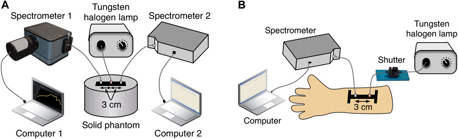
FIGURE 1. Experimental setup for the bbNIRS measurement taken from (A) a tissue phantom and (B) the human forearm. (A) Light source-detector configuration for the phantom measurement. (B) Light source-detector configuration for the human arm measurement.

The second experiment was conducted on the human forearm under the resting state with no stimulation. The experimental protocol was approved by the Institutional Review Board (IRB) of the University of Texas at Arlington. Two healthy adults participated in this experiment. Each subject attended eight measurement sessions on different days, which led to n = 16 measurements. Informed consent was acquired prior to all measurements.

The experimental setup was illustrated in Figure 1B. The bbNIRS system consisted of a tungsten halogen lamp (Model 3900, Illumination Technologies Inc., East Syracuse, NY) and a CCD spectrometer (QE-Pro, Ocean Optics Inc.), both of which were used in the phantom measurements. A flexible probe holder was used to firmly hold the two optical fiber bundles on the subject’s forearm. An optical shutter was also employed to switch on the light only during the exposure time to minimize the tissue heating effect from the broadband light source. An experiment lasted 15 min with a 5 s single light-exposure/data-acquisition time per minute, giving rise to 16 spectra per measurement.

2.4 Monte Carlo Simulations

We also conducted a Monte Carlo (MC) framework that simulated bbNIRS data of the hemodynamic and metabolic states of the exposed tissue. Two physiological conditions were defined within the MC simulation: 1) a baseline state corresponding to the normal resting state of the tissue and 2) a stimulated state where oxygenation and metabolism improved notably. We employed MCmatlab (Marti et al., 2018), an open-source MC program for light propagation in three-dimensional (3-D) media.

Specifically, a (600 × 600 × 300) voxel model corresponding to a (4 × 4 × 2 cm) 3-D volume was first defined as the simulation geometry. The medium that replicates general tissue was considered to be made of water, fat, blood with different oxygen saturation levels, and concentrations of oxCCO and reduced CCO (redCCO). The composition and the optical properties of the medium were defined based on the properties of biological tissues reported in (Jacques, 2013; Jacques et al., 2013). The scattering coefficient μ_s(λ) was considered to be dependent only on the wavelength λ, while the absorption coefficient μ_a(λ) was estimated as the sum of absorption coefficients of all major chromophores composing the medium (Jacques, 2013; Bale et al., 2016). Table 1 summarizes the simulation medium composition of two physiological conditions, while Figure 2 depicts the corresponding absorption coefficient μ_a(λ) (Figure 2A) and the scattering coefficient μ_s(λ) (Figure 2B). The Henyey-Greenstein scattering anisotropy factor g was set to 0.9.

TABLE 1

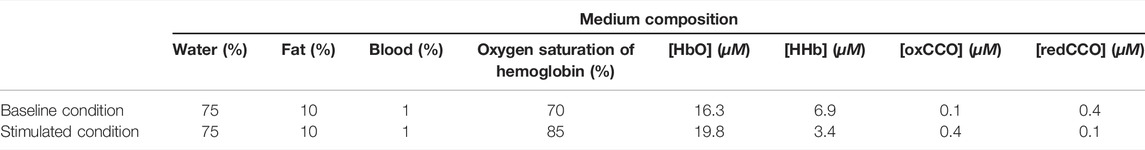
TABLE 1. Summary of the simulation medium composition of two physiological conditions.

FIGURE 2

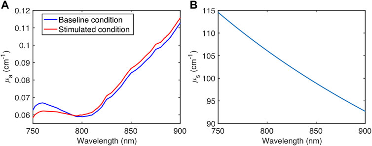
FIGURE 2. (A) Absorption coefficient μ_a(λ) for two physiological conditions and (B) Scattering coefficient μ_s(λ) used in MC simulation.

Note that the concentrations of HbO and HHb were estimated from the predefined percentages of blood and oxygen saturation of hemoglobin, with an average concentration of hemoglobin in blood equal to 150 g/L.

A light source and a detector of 2 cm distance were also defined and placed on the top surface of the 3D voxel model. MC simulation was repeated for different wavelengths within the NIRS range from 780 to 900 nm with 1-nm wavelength resolution, leading to a total of 121 wavelengths, for two physiological conditions. For each MC simulation execution, 50 million (i.e., 5 × 10⁷) photon packets were launched from the light source. The number of photons reaching the detector and their partial pathlengths were recorded for later use when calculating the changes in chromophore concentrations. We repeated the MC simulation 20 times for each wavelength and for each physiological condition. The recorded data were further permuted within each wavelength and each condition 50 times. Gaussian noise was also added to enrich the simulated data. Thus, the whole simulation framework can be considered to generate bbNIRS data of 50 measurements. Each consisted of 20 spectra for each condition, namely, I₀ for the baseline condition and I for the stimulated state.

2.5 Comparison of Measurement or Simulation Versus Theoretical Results of σ_Δ[HbO], σ_Δ[HHb] and σ_Δ[oxCCO]

We sought to compare ${\sigma }_{\mathrm{\Delta }[\text{HbO}]}^T$, ${\sigma }_{\mathrm{\Delta }[\text{HHb}]}^T$ and ${\sigma }_{\mathrm{\Delta }[\text{oxCCO}]}^T$ obtained by the analytical computations versus those by the bbNIRS measurement or MC simulation data, namely, ${\sigma }_{\mathrm{\Delta }[\text{HbO}]}^M$, ${\sigma }_{\mathrm{\Delta }[\text{HHb}]}^M$ and ${\sigma }_{\mathrm{\Delta }[\text{oxCCO}]}^M$. The comparison procedure is depicted in Figure 3. On the one hand, we first calculated Δ[HbO], Δ[HHb], and Δ[oxCCO] from the detected spectra by fitting the modified Beer-Lambert law. Consequently, the standard deviation of measured Δ[HbO], Δ[HHb], and Δ[oxCCO], namely, ${\sigma }_{\mathrm{\Delta }[\text{HbO}]}^M$, ${\sigma }_{\mathrm{\Delta }[\text{HHb}]}^M$ and ${\sigma }_{\mathrm{\Delta }[\text{oxCCO}]}^M$, were then computed. On the other hand, the SNR of the bbNIRS measurements was estimated as $\text{SNR}={\bar{I}}^2/{\sigma }_I^2$, where $\bar{I}$ is the mean spectral intensity and ${\sigma }_I^2$ is the variance of spectra. The SNR curve was then substituted into Eq. 11 to compute ${\sigma }_{\mathrm{\Delta }[\text{HbO}]}^T$, ${\sigma }_{\mathrm{\Delta }[\text{HHb}]}^T$ and ${\sigma }_{\mathrm{\Delta }[\text{oxCCO}]}^T$ from the theoretical analysis, namely, error propagation (EP) caused by system SNR. These steps were repeated for multiple measurements. The measured ${\sigma }_{\mathrm{\Delta }[\text{HbO}]}^M$, ${\sigma }_{\mathrm{\Delta }[\text{HHb}]}^M$ and ${\sigma }_{\mathrm{\Delta }[\text{oxCCO}]}^M$ and the EP by system SNR ${\sigma }_{\mathrm{\Delta }[\text{HbO}]}^T$, ${\sigma }_{\mathrm{\Delta }[\text{HHb}]}^T$ and ${\sigma }_{\mathrm{\Delta }[\text{oxCCO}]}^T$ were finally compared to verify/confirm the accuracy of the quantitative analysis.

FIGURE 3

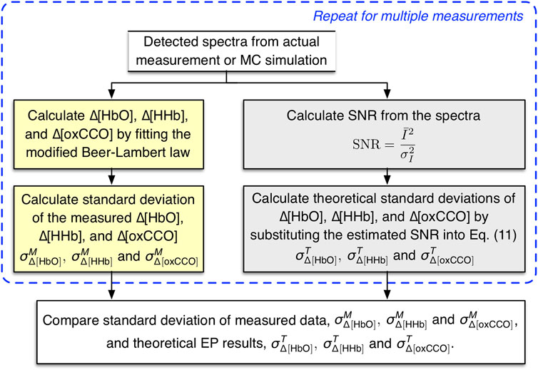
FIGURE 3. Procedure for comparing ${\sigma }_{\mathrm{\Delta }[\text{HbO}]}^M$, ${\sigma }_{\mathrm{\Delta }[\text{HHb}]}^M$ and ${\sigma }_{\mathrm{\Delta }[\text{oxCCO}]}^M$ obtained from the bbNIRS measurement or MC-simulation data (yellow-shaded steps) and the theoretical EP ${\sigma }_{\mathrm{\Delta }[\text{HbO}]}^T$, ${\sigma }_{\mathrm{\Delta }[\text{HHb}]}^T$ and ${\sigma }_{\mathrm{\Delta }[\text{oxCCO}]}^T$ calculated using system SNR (gray-shaded steps).

3 Results

3.1 Standard Deviation of Δ[HbO], Δ[HHb] and Δ[oxCCO] Derived From Error Propagation Analysis and Actual Measurement Data

Figure 4 presents comparative results of ${\sigma }_{\mathrm{\Delta }[\text{HbO}]}^M$, ${\sigma }_{\mathrm{\Delta }[\text{HHb}]}^M$ and ${\sigma }_{\mathrm{\Delta }[\text{oxCCO}]}^M$ obtained from the measurement data and ${\sigma }_{\mathrm{\Delta }[\text{HbO}]}^T$, ${\sigma }_{\mathrm{\Delta }[\text{HHb}]}^T$ and ${\sigma }_{\mathrm{\Delta }[\text{oxCCO}]}^T$ from the theoretical analysis (Eq. 11). Specifically, the mean and standard deviation spectra of SNR estimated from the detected optical spectra of multiple measurements are depicted in Figures 4A–C, taken from (A) spectrometer 1 in the phantom measurement, (B) spectrometer 2 also in the concurrent phantom experiment, and (C) the human forearm measurement, respectively. Consequently, Figures 4D–F show ${\sigma }_{\mathrm{\Delta }[\text{HbO}]}^M$, ${\sigma }_{\mathrm{\Delta }[\text{HHb}]}^M$ and ${\sigma }_{\mathrm{\Delta }[\text{oxCCO}]}^M$ computed/derived from the measured optical spectra (red bars) versus ${\sigma }_{\mathrm{\Delta }[\text{HbO}]}^T$, ${\sigma }_{\mathrm{\Delta }[\text{HHb}]}^T$ and ${\sigma }_{\mathrm{\Delta }[\text{oxCCO}]}^T$ by theoretically derived EP (blue bars).

FIGURE 4

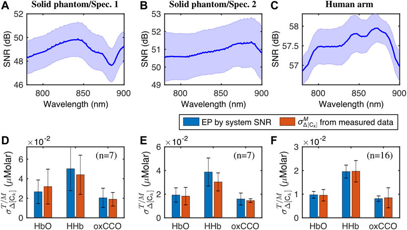
FIGURE 4. The top row depicts the mean and standard deviation of SNR spectra from (A) the solid phantom measurement with spectrometer 1, (B) the solid phantom measurement with spectrometer 2, and (C) the human forearm measurement. The bottom row shows the ${\sigma }_{\mathrm{\Delta }[\text{HbO}]}^T$, ${\sigma }_{\mathrm{\Delta }[\text{HHb}]}^T$ and ${\sigma }_{\mathrm{\Delta }[\text{oxCCO}]}^T$ obtained from the error propagation analysis (blue bars) and ${\sigma }_{\mathrm{\Delta }[\text{HbO}]}^M$, ${\sigma }_{\mathrm{\Delta }[\text{HHb}]}^M$ and ${\sigma }_{\mathrm{\Delta }[\text{oxCCO}]}^M$ from the measurement data (red bars) for (D) the solid phantom measurement with spectrometer 1, (E) the solid phantom measurement with spectrometer 2, and (F) the human forearm measurement. Error bars indicate the standard error of the mean of each group.

As seen in Figures 4A–C, the spectral shapes of SNR appeared to be different from one another. This observation is understandable since each of them was obtained from a specific bbNIRS system. Specifically, SNR spectra in Figures 4A,B were derived from the data collected concurrently by two spectrometers under the same experimental conditions, and the differences in the spectral sensitivity of these two spectrometers led to distinctive SNR spectral shapes. The bbNIRS data from the human arm experiment (Figure 4C) were acquired by the same QE-Pro spectrometer as in the solid phantom/spectrometer 2 case (Figure 4B). However, different exposure times for data acquisition (5 vs. 1 s) resulted in un-identical SNR spectra.

Despite the variations of SNR spectra, no significant differences were found between measured ${\sigma }_{\mathrm{\Delta }[\text{HbO}]}^M$, ${\sigma }_{\mathrm{\Delta }[\text{HHb}]}^M$ and ${\sigma }_{\mathrm{\Delta }[\text{oxCCO}]}^M$ versus ${\sigma }_{\mathrm{\Delta }[\text{HbO}]}^T$, ${\sigma }_{\mathrm{\Delta }[\text{HHb}]}^T$ and ${\sigma }_{\mathrm{\Delta }[\text{oxCCO}]}^T$ calculated directly from the EP analysis (Eq. 11) in all the cases. Specifically, the human forearm measurement led to a high SNR range (i.e., 57–58 dB) (Figure 4C) and low ${\sigma }_{\mathrm{\Delta }[\text{HbO}]}^{M/T}$, ${\sigma }_{\mathrm{\Delta }[\text{HHb}]}^{M/T}$ and ${\sigma }_{\mathrm{\Delta }[\text{oxCCO}]}^{M/T}$ (Figure 4F) because of a prolonged exposure time for data acquisition (5 s). The same spectrometer was used in the solid phantom measurement, but a shorter exposure time of 1 s resulted in a reduced SNR range of the measured data (Figure 4B). The measured data from both spectrometers in the solid phantom measurement led to higher ${\sigma }_{\mathrm{\Delta }[\text{HbO}]}^{M/T}$, ${\sigma }_{\mathrm{\Delta }[\text{HHb}]}^{M/T}$ and ${\sigma }_{\mathrm{\Delta }[\text{oxCCO}]}^{M/T}$ compared to the human arm measurement.

3.2 Standard Deviation of Δ[HbO], Δ[HHb] and Δ[oxCCO] Derived From Error Propagation Analysis and MC Simulation Data

We also compared the uncertainties of Δ[HbO], Δ[HHb] and Δ[oxCCO] obtained from the MC simulation and EP results derived from the corresponding SNR. Figure 5A depicts the mean and standard deviation spectra of SNR of the MC simulation, while Figure 5B presents the comparative results of ${\sigma }_{\mathrm{\Delta }[\text{HbO}]}^T$, ${\sigma }_{\mathrm{\Delta }[\text{HHb}]}^T$ and ${\sigma }_{\mathrm{\Delta }[\text{oxCCO}]}^T$ derived from the proposed EP calculation (blue bars) and ${\sigma }_{\mathrm{\Delta }[\text{HbO}]}^M$, ${\sigma }_{\mathrm{\Delta }[\text{HHb}]}^M$ and ${\sigma }_{\mathrm{\Delta }[\text{oxCCO}]}^M$ computed from the MC simulation data (red bars). One more time, no significant difference was found in the standard deviation of chromophore concentration changes calculated from the MC simulation data and from the EP analysis. The SNR of the MC simulation (Figure 5A) was lower than those of the real measurements (Figures 4A–C) due to the MC simulation settings. Nevertheless, it could be improved by having a larger tissue volume and a larger number of photons. Generally, the higher the average SNR of the measurement system, the lower the error propagates to the calculated changes in chromophore concentration.

FIGURE 5

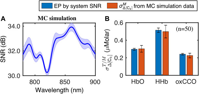
FIGURE 5. (A) Mean and standard deviation of SNR spectra from MC simulation data and (B) Comparison of ${\sigma }_{\mathrm{\Delta }[\text{HbO}]}^T$, ${\sigma }_{\mathrm{\Delta }[\text{HHb}]}^T$ and ${\sigma }_{\mathrm{\Delta }[\text{oxCCO}]}^T$ obtained from the error propagation analysis (blue bars) and ${\sigma }_{\mathrm{\Delta }[\text{HbO}]}^M$, ${\sigma }_{\mathrm{\Delta }[\text{HHb}]}^M$ and ${\sigma }_{\mathrm{\Delta }[\text{oxCCO}]}^M$ from the MC simulation data (red bars). Error bars indicate the standard error of the mean of each group.

These results confirmed that the analytically derived expressions of ${\sigma }_{\mathrm{\Delta }[\text{HbO}]}^T$, ${\sigma }_{\mathrm{\Delta }[\text{HHb}]}^T$ and ${\sigma }_{\mathrm{\Delta }[\text{oxCCO}]}^T$ matched well with those obtained from true experiments and MC simulations. Thus, the theoretical analysis of EP (i.e., Eq. 11) can be used as a quick reference or prediction to estimate measurement errors or accuracy of Δ[HbO], Δ[HHb] and Δ[oxCCO] given an SNR of a bbNIRS system. In the following two sub-sections, we applied the EP analysis to examine the influence of wavelength selection and spectral range of bbNIRS on the variance of chromophore concentration changes. Note that the values of the optical pathlength L(λ_i) = r ×DPF(λ_i) can be estimated by diffusion theory, as given in refs. Patterson et al. (1989), Sevick et al. (1991).

3.3 Influence of Selection of Wavelengths on ${\sigma }_{\mathrm{\Delta }[\text{HbO}]}^T$, ${\sigma }_{\mathrm{\Delta }[\text{HHb}]}^T$ and ${\sigma }_{\mathrm{\Delta }[\text{oxCCO}]}^T$

We further illustrated how wavelength selections would affect the SNR-derived ${\sigma }_{\mathrm{\Delta }[\text{HbO}]}^T$, ${\sigma }_{\mathrm{\Delta }[\text{HHb}]}^T$ and ${\sigma }_{\mathrm{\Delta }[\text{oxCCO}]}^T$. Theoretically, to quantify values of Δ[HbO], Δ[HHb] and Δ[oxCCO], at least three wavelengths are required for NIRS measurements. However, because of the spectrally smooth feature of CCO, it is rather challenging to accurately quantify Δ[oxCCO]. A small number of wavelengths typically leads to inaccurate quantification of Δ[HbO], Δ[HHb] and Δ[oxCCO]. To address this problem, broadband spectroscopy with a full wavelength range of measurement has been suggested and utilized in recent studies, such as 740–900 nm in studies of (Heekeren et al., 1999; Kolyva et al., 2012; Kolyva et al., 2014; Wang X. et al., 2016), 770–905 nm in publications of (Bale et al., 2014, 2019), and 780–900 nm in reports of (Heekeren et al., 1999; Kolyva et al., 2012; Kolyva et al., 2014; Giannoni et al., 2020). Since a large number of wavelengths required in bbNIRS can be an obstacle for development of a compact or portable system (Chitnis et al., 2016), various studies made efforts to find an optimal set of wavelengths to minimize the number of required wavelengths while keeping satisfactory accuracy for the quantifications (Arifler et al., 2015). Bale et al. (2016) reviewed existing clinical NIRS systems and summarized different broadband ranges or wavelength combinations used in these systems. We followed this review paper and selected/updated some representative wavelength ranges or wavelength combinations to illustrate how wavelength selections affect the accuracy of the calculated chromophore concentration changes. Table 2 summarizes different ranges of wavelengths or optimal wavelength sets that have been in the literature to estimate Δ[HbO], Δ[HHb] and Δ[oxCCO]. Note that Sudakou et al. (2019) performed a Monte Carlo study to estimate Δ[CCO] uncertainty using 16 consecutive wavelengths separated by an equal interval of 12.5 nm with a moving spectral window covering from 650 to 950 nm. However, such a study focused on the time-resolved NIRS and utilized a 3-layer model (scalp, skull, and brain). Consequently, the error propagation analysis included the moment method for analyzing time-resolved statistical uncertainty and multilayer considerations. Thus, the variance of Δ[CCO] and respective analysis by Sudakou et al. were distinct from this work and thus excluded in Table 2 for comparison.

TABLE 2

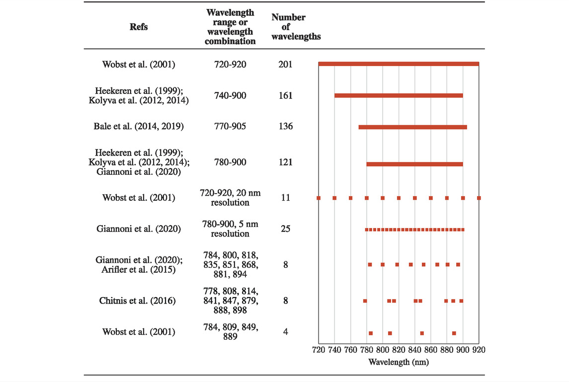
TABLE 2. Summary of different ranges of wavelengths or optimal wavelength combination sets.

Figure 6 depicts ${\sigma }_{\mathrm{\Delta }[\text{HbO}]}^T$, ${\sigma }_{\mathrm{\Delta }[\text{HHb}]}^T$ and ${\sigma }_{\mathrm{\Delta }[\text{oxCCO}]}^T$ calculated using the EP analytical expression (i.e., Eq. 11) for different broadband wavelength ranges (Figure 6A) or different wavelength combinations (Figure 6B). Selections of the ranges or combinations were based on the exact values given in Table 2. In these calculations, we temporally assumed a constant SNR value across all wavelengths and performed the EP calculation for different SNR values varying from 20 to 60 dB (equivalently, noise level (NL) being from 10% to 0.1%). As shown in Figure 6A, the broadest bandwidth of 720–920 nm (with 201 wavelengths) led to the smallest ${\sigma }_{\mathrm{\Delta }[\text{HbO}]}^T$, ${\sigma }_{\mathrm{\Delta }[\text{HHb}]}^T$ and ${\sigma }_{\mathrm{\Delta }[\text{oxCCO}]}^T$, while the narrowest range of 780–900 nm (with 121 wavelengths) resulted in the largest EP in respective concentrations, especially for the case of Δ[HHb]. In the case of using a limited number of wavelengths, calculated ${\sigma }_{\mathrm{\Delta }[\text{HbO}]}^T$, ${\sigma }_{\mathrm{\Delta }[\text{HHb}]}^T$ and ${\sigma }_{\mathrm{\Delta }[\text{oxCCO}]}^T$ increased noticeably, even by visual comparison between Figures 6A,B. For instance, at an SNR of 40 dB, EP varied from 0.08–0.12 μM for Δ[HbO] and from 0.05–0.1 μM for Δ[oxCCO] when using all wavelengths of bbNIRS, while the EP increased by at least four times when using a limited number of wavelengths; namely, EP varied from 0.25 to 0.64 μM for Δ[HbO] and from 0.2 to 0.5 μM for Δ[oxCCO]. In most cases, the more wavelengths used to calculate concentration changes of each chromophore, the smaller error propagation in the results. For the case that the same number of wavelengths was used (e.g., 8 wavelengths used in (Arifler et al., 2015; Giannoni et al., 2020) or in (Chitnis et al., 2016)), the distinct wavelength combinations led to different error propagation results. For instance, these two sets of 8 wavelengths led to approximate ${\sigma }_{\mathrm{\Delta }[\text{HbO}]}^T$ value but distinct ${\sigma }_{\mathrm{\Delta }[\text{HHb}]}^T$ and ${\sigma }_{\mathrm{\Delta }[\text{oxCCO}]}^T$ (green and pink curves in Figure 6B).

FIGURE 6

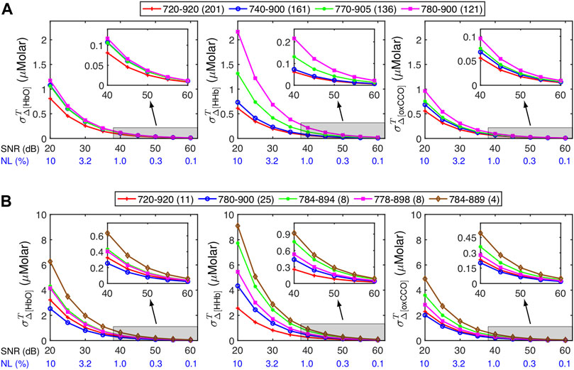
FIGURE 6. Influence of different spectral ranges of wavelengths or wavelength combinations on ${\sigma }_{\mathrm{\Delta }[\text{HbO}]}^T$, ${\sigma }_{\mathrm{\Delta }[\text{HHb}]}^T$ and ${\sigma }_{\mathrm{\Delta }[\text{oxCCO}]}^T$ for a bbNIRS system. (A) ${\sigma }_{\mathrm{\Delta }[\text{HbO}]}^T$, ${\sigma }_{\mathrm{\Delta }[\text{HHb}]}^T$ and ${\sigma }_{\mathrm{\Delta }[\text{oxCCO}]}^T$ obtained by using a broad range of bandwidths. The numbers in the legend labels correspond to the spectral bandwidth, while the number within the parenthesis is the total number of wavelengths used to compute ${\sigma }_{\mathrm{\Delta }[\text{HbO}]}^T$, ${\sigma }_{\mathrm{\Delta }[\text{HHb}]}^T$ and ${\sigma }_{\mathrm{\Delta }[\text{oxCCO}]}^T$. (B) ${\sigma }_{\mathrm{\Delta }[\text{HbO}]}^T$, ${\sigma }_{\mathrm{\Delta }[\text{HHb}]}^T$ and ${\sigma }_{\mathrm{\Delta }[\text{oxCCO}]}^T$ obtained by using different wavelength combinations. The numbers of the legend labels correspond to the minimum and maximum wavelength values; the numbers in the parentheses are the total number of wavelengths used to compute ${\sigma }_{\mathrm{\Delta }[\text{HbO}]}^T$, ${\sigma }_{\mathrm{\Delta }[\text{HHb}]}^T$ and ${\sigma }_{\mathrm{\Delta }[\text{oxCCO}]}^T$.

Note that the results presented here should be considered as approximate references to roughly estimate ${\sigma }_{\mathrm{\Delta }[\text{HbO}]}^T$, ${\sigma }_{\mathrm{\Delta }[\text{HHb}]}^T$ and ${\sigma }_{\mathrm{\Delta }[\text{oxCCO}]}^T$ measured from a bbNIRS system with an approximate SNR varying within the given range. For a specific bbNIRS system with a known SNR spectrum, more precise estimations of error propagation in calculating chromophore concentration changes can be carried out by substituting the system’s SNR spectrum into Eq. 11 according to the respective wavelength ranges or wavelength combinations.

3.4 Influence of Spectral Bandwidth in bbNIRS on ${\sigma }_{\mathrm{\Delta }[\text{HbO}]}^T$, ${\sigma }_{\mathrm{\Delta }[\text{HHb}]}^T$ and ${\sigma }_{\mathrm{\Delta }[\text{oxCCO}]}^T$

As revealed in Figure 6, using a broader wavelength range in bbNIRS led to significantly smaller ${\sigma }_{\mathrm{\Delta }[\text{HbO}]}^T$, ${\sigma }_{\mathrm{\Delta }[\text{HHb}]}^T$ and ${\sigma }_{\mathrm{\Delta }[\text{oxCCO}]}^T$. However, to our knowledge, no study has reported the spectral-bandwidth dependence of variance in calculating chromophore concentration changes. In the following, we demonstrate how selections of spectral ranges would impact the variances of Δ[HbO], Δ[HHb] and Δ[oxCCO] based on the derived Eq. 11.

As an example, three panels of Figure 7 depict ${\sigma }_{\mathrm{\Delta }[\text{HbO}]}^T$, ${\sigma }_{\mathrm{\Delta }[\text{HHb}]}^T$ and ${\sigma }_{\mathrm{\Delta }[\text{oxCCO}]}^T$ with different spectral ranges at the SNR of 40 dB (for simplicity). Each curve in each panel plots EP dependence on spectral ranges with a starting wavelength of λ_i and an ending wavelength of λ_j, where λ_i varies from 700 to 800 nm in a step of 10 nm (as noted on top of the figures), and λ_j corresponds to the x-axis from 820 to 920 nm in each panel, also in a step of 10 nm. For instance, the red curves represent ${\sigma }_{\mathrm{\Delta }[\text{HbO}]}^T$, ${\sigma }_{\mathrm{\Delta }[\text{HHb}]}^T$ and ${\sigma }_{\mathrm{\Delta }[\text{oxCCO}]}^T$ obtained with spectral ranges of 700–820 nm, 700–830 nm, … , and finally 700–920 nm. Similarly, the orange curves depict EP of respective concentration changes within wavelength ranges of 710–820 nm, 710–830 nm, … , 710–920 nm.

FIGURE 7

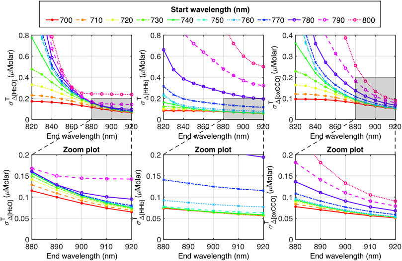
FIGURE 7. Top row: Dependance of ${\sigma }_{\mathrm{\Delta }[\text{HbO}]}^T$, ${\sigma }_{\mathrm{\Delta }[\text{HHb}]}^T$ and ${\sigma }_{\mathrm{\Delta }[\text{oxCCO}]}^T$, obtained by the derived EP expressions, on different spectral ranges with a spectral SNR of 40 dB. Each curve corresponds to a start wavelength of the bbNIRS spectral range as marked in the top legend, while the x-axis corresponds to the end wavelength of the bbNIRS spectral range. Bottom row: Respective zoomed plots of the gray areas shown in the top row.

The three zoomed panels in Figure 7 provide more detailed information. Specifically, ${\sigma }_{\mathrm{\Delta }[\text{HbO}]}^T$ varied around or below 0.15 μM if the starting λ_i was shorter than 780 nm and the ending λ_j equal to or longer than 880 nm. Meanwhile, both ${\sigma }_{\mathrm{\Delta }[\text{HHb}]}^T$ and ${\sigma }_{\mathrm{\Delta }[\text{oxCCO}]}^T$ had a large reduction if the start λ_i was shorter than 760 nm. Overall, the spectral range of 760–890 nm can be considered as an optimal range to minimize variances of calculated Δ[HbO], Δ[HHb] and Δ[oxCCO] in bbNIRS. Wider spectral ranges still can reduce ${\sigma }_{\mathrm{\Delta }[\text{HbO}]}^T$, ${\sigma }_{\mathrm{\Delta }[\text{HHb}]}^T$ and ${\sigma }_{\mathrm{\Delta }[\text{oxCCO}]}^T$, but the improvement may be non-significant.

4 Discussions

Accurate quantifications of Δ[HbO], Δ[HHb] and Δ[oxCCO] are of importance in most NIRS-based studies since they characterize and reflect hemodynamic and metabolic activities of the tissue under specific physiology. Since the values of Δ[HbO], Δ[HHb] and Δ[oxCCO] are deduced from measured optical densities at multiple wavelengths, the accuracy of the calculated results is inherently affected by the measurement variances or SNR of the hardware. Previous studies included analyses on the uncertainties of Δ[HbO], Δ[HHb] and Δ[oxCCO] caused by variances of extinction coefficients (Kim and Liu, 2007) or different wavelength combinations (Funane et al., 2009; Sudakou et al., 2019; Caredda et al., 2020). However, literature shows few publications that quantify the influence of SNR on variances of Δ[HbO], Δ[HHb] and Δ[oxCCO] derived from bbNIRS.

In this study, we performed the error propagation analysis to derive analytical variances of Δ[HbO], Δ[HHb] and Δ[oxCCO] caused by uncertainties of the bbNIRS measurement system. The derivation of EP of respective concentration changes was achieved by fitting the measured data using the least-squares method (York, 1966). The analytical expressions and experimental/MC-simulation results were compared and confirmed statistically non-significant difference between the theoretical and measurement-based variances of chromophore concentration changes. Experimental results also indicated that the larger the SNR of a bbNIRS system, the smaller the quantified ${\sigma }_{\mathrm{\Delta }[\text{HbO}]}^T$, ${\sigma }_{\mathrm{\Delta }[\text{HHb}]}^T$ and ${\sigma }_{\mathrm{\Delta }[\text{oxCCO}]}^T$ (Figure 4D–F). Note that in both actual experiments presented in Section 2.3 and Section 3.1, we tried to enhance the SNR of the bbNIRS system by warming up the system to reach a stable state before acquiring the data. For a new or self-designed bbNIRS system, the thermal and electrical fluctuations of the system over time should be first investigated to ensure the required warm-up time to reach the desired system stability.

In the case of bbNIRS, a large number of wavelengths with different spectral ranges or bandwidths have been considered when calculating the chromophore concentration changes (Heekeren et al., 1999; Kolyva et al., 2012; Bale et al., 2014; Kolyva et al., 2014; Wang X. et al., 2016; Bale et al., 2019; Giannoni et al., 2020), as summarized in Table 2. The results from our analysis clearly demonstrated that ${\sigma }_{\mathrm{\Delta }[\text{HbO}]}^T$, ${\sigma }_{\mathrm{\Delta }[\text{HHb}]}^T$ and ${\sigma }_{\mathrm{\Delta }[\text{oxCCO}]}^T$ were relatively small, varying from 0.07 to 0.1 μM for the wavelength range of 720–900 nm at an SNR of 40 dB. The bandwidth of the spectral ranges of bbNIRS also affect the variance of calculated Δ[HbO], Δ[HHb] and Δ[oxCCO]. Accordingly, Figure 7 may serve as a useful guide or predictor to select an optimal spectral range/bandwidth for accurate determination of changes in chromophore concentrations by a bbNIRS measurement device.

It is worth noting that although the results presented in Figures 6, 7 were calculated using a constant SNR value, this does not imply that the derived EP calculation cannot be applied to a real bbNIRS system where SNR has a spectral feature depending on the wavelength. We presented Figures 6, 7 for the purpose of giving the reader an approximated amount/order of ${\sigma }_{\mathrm{\Delta }[\text{HbO}]}^T$, ${\sigma }_{\mathrm{\Delta }[\text{HHb}]}^T$ and ${\sigma }_{\mathrm{\Delta }[\text{oxCCO}]}^T$ caused by a certain SNR level. For instance, in our previous studies on the effects of transcranial photobiomodulation (tPBM) (Wang et al., 2017; Pruitt et al., 2020), we employed the same bbNIRS system as that used in this study for the human arm measurement (Figures 4C, F). As seen in these two figures, SNRs in the wavelength range of 780–900 nm would be around 57–58 dB. With such a high SNR level, the respective EP were estimated or predicted to be about 0.01 μM for Δ[HbO], 0.02 μM for Δ[HHb], and less than 0.01 μM for Δ[oxCCO]. Meanwhile, the changes in [HbO] and [CCO] concentration induced by tPBM were about 5 and 0.6 μM, respectively (Wang et al., 2017; Pruitt et al., 2020). Compared to these actual measured values of Δ[HbO] and Δ[oxCCO], the EP caused by the measurement SNR were minimal. In particular, it is more critical to be able to estimate or predict ${\sigma }_{\mathrm{\Delta }[\text{oxCCO}]}^T$ values and consequently to design optimal wavelength range, spectral bandwidth, and light exposure time. In this way, the weaker signal from less concentrated Δ[oxCCO] in tissue can be still correctly determined without being shadowed or overwhelmed by much stronger signals from Δ[HbO] and Δ[HHb].

Some efforts have also been carried out to select a limited number of wavelengths to lessen the complexity of the spectral hardware or system but still ensure the calculation or quantification accuracy (Wobst et al., 2001; Arifler et al., 2015; de Roever et al., 2018; Caredda et al., 2020). One objective of such studies was to design wearable NIRS systems (Wyser et al., 2017; Chitnis et al., 2016). However, based on the results of error propagation analysis obtained in Section 3.3, limiting the wavelength number would lead to more uncertainties in the calculated Δ[HbO], Δ[HHb] and Δ[oxCCO]. For instance, at an SNR of 40 dB, σ_Δ[HbO], σ_Δ[HHb] and σ_Δ[oxCCO] varied from 0.2 to 0.9 μM if a limited number of wavelengths was used (Figure 6B), compared to 0.07–0.1 μM for the full bandwidth of 720–920 nm (Figure 6A, red curve). Moreover, distinct wavelength combinations led to different error propagation results. Thus, one may want to estimate the SNR-derived variance of Δ[HbO], Δ[HHb] and Δ[oxCCO] using different available wavelength combinations before deciding the optimal set that leads to minimal error propagation. Additional data processing or fitting steps, such as the genetic algorithm (Arifler et al., 2015), may be added to help improve the quantification accuracy. If such a step is taken, further error analysis should be carried out to consider the contribution of additional steps in the EP calculation.

Last, to better understand the scientific reasoning why the variance of chromophore concentration changes depends on the spectral range and wavelength selection, we performed a mathematical expansion of the EP matrix inverse (Eq. 11), as given in Appendix. The final results demonstrate that the variance for each of Δ[HbO], Δ[HHb], and Δ[oxCCO] is computed from the extinction coefficients of all three chromophores at given multiple wavelengths. Since these expressions are highly wavelength dependent and extinction coefficient nested, it is impossible to directly infer an optimal spectral bandwidth or wavelength combination that can lead to minimal error propagation. However, the knowledge learned from these equations is that the device-driven errors for Δ[HbO], Δ[HHb], and Δ[oxCCO] in a bbNIRS system depend closely on the extinction coefficient spectra of the three chromophores. Also, it might be theoretically possible to optimally select wavelengths by maximizing Eq. A2 and minimizing Eqs A4–A6 simultaneously for a given bandwidth. However, the latter point is beyond the scope of this work and needs to be investigated in future studies.

5 Conclusion

This study investigated the influence of SNR on variance of Δ[HbO], Δ[HHb] and Δ[oxCCO] measured by a bbNIRS device or system. Since all measured data contain inevitable uncertainties caused by thermal or electrical fluctuations or disturbance of the devices, such uncertainties or errors must impact the accuracy of the calculated Δ[HbO], Δ[HHb] and Δ[oxCCO]. Based on error propagation analysis, we derived analytical expressions of EP for all three chromophore concentrations depending on the SNR spectral curve of the bbNIRS measurement system. To compare the quantitative results and those obtained from actual bbNIRS measurements, we performed two sets of experiments on a solid tissue phantom and the human forearm using two bbNIRS systems. We also introduced an MC framework mimicking a set of bbNIRS measurements with two predefined physiological states of tissue. Both experimental and MC simulation results statistically confirmed and supported the analytical expression of the variance or EP of Δ[HbO], Δ[HHb], and Δ[oxCCO] derived in this work. Further analyses were further performed to demonstrate effects of the wavelength selection, spectral range and bandwidth, as well as spectral locations on the accuracy of the computed Δ[HbO], Δ[HHb], and Δ[oxCCO]. The presented work or results can be a helpful reference to guide optimal selections of wavelength ranges and different wavelength combinations for minimal variances of Δ[HbO], Δ[HHb], and Δ[oxCCO] in an actual bbNIRS system.

Data Availability Statement

The original contributions presented in the study are included in the article/supplementary material, further inquiries can be directed to the corresponding author.

Ethics Statement

The studies involving human participants were reviewed and approved by The Institutional Review Board of the University of Texas at Arlington. The patients/participants provided their written informed consent to participate in this study.

Author Contributions

NT derived theoretical expressions, performed both phantom experiments and MC simulations, analyzed the data, interpreted the results, and prepared the manuscript. SS assisted and discussed theoretical formulation. SK performed human forearm measurements. XW discussed data analysis and the results. HL initiated and supervised the study, discussed and interpreted the results, as well as reviewed and revised the manuscript. All authors reviewed and approved the manuscript.

Funding

This work was supported in part by the National Institute of Mental Health/National Institutes of Health under the BRAIN Initiative (RF1MH114285).

Conflict of Interest

The authors declare that the research was conducted in the absence of any commercial or financial relationships that could be construed as a potential conflict of interest.

Publisher’s Note

All claims expressed in this article are solely those of the authors and do not necessarily represent those of their affiliated organizations, or those of the publisher, the editors and the reviewers. Any product that may be evaluated in this article, or claim that may be made by its manufacturer, is not guaranteed or endorsed by the publisher.

References

Alfano, R. R., Sordillo, L., Pu, Y., and Shi, L. (2018). Deep Optical Imaging Of Tissue With Less Scattering In The Second, Third And Fourth NIR Spectral Windows Using Supercontinuum And Other Laser Coherent Light Sources. (U.S. Patent No. 10,123,705). Washington, DC: U.S. Patent and Trademark Office.

Google Scholar

Arifler, D., Zhu, T., Madaan, S., and Tachtsidis, I. (2015). Optimal Wavelength Combinations for Near-Infrared Spectroscopic Monitoring of Changes in Brain Tissue Hemoglobin and Cytochrome C Oxidase Concentrations. Biomed. Opt. Express 6, 933–947. doi:10.1364/boe.6.000933

PubMed Abstract | CrossRef Full Text | Google Scholar

Bale, G., Elwell, C. E., and Tachtsidis, I. (2016). From Jöbsis to the Present Day: a Review of Clinical Near-Infrared Spectroscopy Measurements of Cerebral Cytochrome-C-Oxidase. J. Biomed. Opt. 21, 091307. doi:10.1117/1.JBO.21.9.091307

PubMed Abstract | CrossRef Full Text | Google Scholar

Bale, G., Mitra, S., de Roever, I., Sokolska, M., Price, D., Bainbridge, A., et al. (2019). Oxygen Dependency of Mitochondrial Metabolism Indicates Outcome of Newborn Brain Injury. J. Cereb. Blood Flow. Metab. 39, 2035–2047. doi:10.1177/0271678x18777928

PubMed Abstract | CrossRef Full Text | Google Scholar

Bale, G., Mitra, S., Meek, J., Robertson, N., and Tachtsidis, I. (2014). A New Broadband Near-Infrared Spectroscopy System for In-Vivo Measurements of Cerebral Cytochrome-C-Oxidase Changes in Neonatal Brain Injury. Biomed. Opt. Express 5, 3450–3466. doi:10.1364/boe.5.003450

PubMed Abstract | CrossRef Full Text | Google Scholar

Bevington, P. R., Robinson, D. K., Blair, J. M., Mallinckrodt, A. J., and McKay, S. (1993). Data Reduction and Error Analysis for the Physical Sciences. Comput. Phys. 7, 415–416. doi:10.1063/1.4823194

CrossRef Full Text | Google Scholar

Bigio, I. J., and Fantini, S. (2016). Quantitative Biomedical Optics: Theory, Methods, and Applications. Cambridge: Cambridge University Press.

Google Scholar

Boas, D. A., Elwell, C. E., Ferrari, M., and Taga, G. (2014). Twenty Years of Functional Near-Infrared Spectroscopy: Introduction for the Special Issue. NeuroImage 85, 1–5. doi:10.1016/j.neuroimage.2013.11.033

PubMed Abstract | CrossRef Full Text | Google Scholar

Boas, D. A., and Franceschini, M. A. (2011). Haemoglobin Oxygen Saturation as a Biomarker: The Problem and a Solution. Phil. Trans. R. Soc. A 369, 4407–4424. doi:10.1098/rsta.2011.0250

PubMed Abstract | CrossRef Full Text | Google Scholar

Caredda, C., Mahieu-Williame, L., Sablong, R., Sdika, M., Guyotat, J., and Montcel, B. (2020). Optimal Spectral Combination of a Hyperspectral Camera for Intraoperative Hemodynamic and Metabolic Brain Mapping. Appl. Sci. 10, 5158. doi:10.3390/app10155158

CrossRef Full Text | Google Scholar

Cerussi, A. E., Tanamai, V. W., Hsiang, D., Butler, J., Mehta, R. S., and Tromberg, B. J. (2011). Diffuse Optical Spectroscopic Imaging Correlates with Final Pathological Response in Breast Cancer Neoadjuvant Chemotherapy. Phil. Trans. R. Soc. A 369, 4512–4530. doi:10.1098/rsta.2011.0279

PubMed Abstract | CrossRef Full Text | Google Scholar

Chitnis, D., Airantzis, D., Highton, D., Williams, R., Phan, P., Giagka, V., et al. (2016). Towards a Wearable Near Infrared Spectroscopic Probe for Monitoring Concentrations of Multiple Chromophores in Biological Tissue In Vivo. Rev. Sci. Instrum. 87, 065112. doi:10.1063/1.4954722

PubMed Abstract | CrossRef Full Text | Google Scholar

de Roever, I., Bale, G., Mitra, S., Meek, J., Robertson, N. J., and Tachtsidis, I. (2018). Investigation of the Pattern of the Hemodynamic Response as Measured by Functional Near-Infrared Spectroscopy (fNIRS) Studies in Newborns, Less Than a Month Old: A Systematic Review. Front. Hum. Neurosci. 12, 371. doi:10.3389/fnhum.2018.00371

PubMed Abstract | CrossRef Full Text | Google Scholar

Durduran, T., Choe, R., Baker, W. B., and Yodh, A. G. (2010). Diffuse Optics for Tissue Monitoring and Tomography. Rep. Prog. Phys. 73, 076701. doi:10.1088/0034-4885/73/7/076701

PubMed Abstract | CrossRef Full Text | Google Scholar

Ferrari, M., Muthalib, M., and Quaresima, V. (2011). The Use of Near-Infrared Spectroscopy in Understanding Skeletal Muscle Physiology: Recent Developments. Phil. Trans. R. Soc. A 369, 4577–4590. doi:10.1098/rsta.2011.0230

PubMed Abstract | CrossRef Full Text | Google Scholar

Funane, T., Atsumori, H., Sato, H., Kiguchi, M., and Maki, A. (2009). Relationship between Wavelength Combination and Signal-To-Noise Ratio in Measuring Hemoglobin Concentrations Using Visible or Near-Infrared Light. Opt. Rev. 16, 442–448. doi:10.1007/s10043-009-0084-6

CrossRef Full Text | Google Scholar

Giannoni, L., Lange, F., and Tachtsidis, I. (2020). Investigation of the Quantification of Hemoglobin and Cytochrome-C-Oxidase in the Exposed Cortex with Near-Infrared Hyperspectral Imaging: A Simulation Study. J. Biomed. Opt. 25–25. doi:10.1117/1.JBO.25.4.046001

CrossRef Full Text | Google Scholar

Goodman, L. A. (1960). On the Exact Variance of Products. J. Am. Stat. Assoc. 55, 708–713. doi:10.1080/01621459.1960.10483369

CrossRef Full Text | Google Scholar

Hamaoka, T., McCully, K. K., Niwayama, M., and Chance, B. (2011). The Use of Muscle Near-Infrared Spectroscopy in Sport, Health and Medical Sciences: Recent Developments. Phil. Trans. R. Soc. A 369, 4591–4604. doi:10.1098/rsta.2011.0298

PubMed Abstract | CrossRef Full Text | Google Scholar

Heekeren, H. R., Kohl, M., Obrig, H., Wenzel, R., von Pannwitz, W., Matcher, S. J., et al. (1999). Noninvasive Assessment of Changes in Cytochrome-C Oxidase Oxidation in Human Subjects during Visual Stimulation. J. Cereb. Blood Flow. Metab. 19, 592–603. doi:10.1097/00004647-199906000-00002

PubMed Abstract | CrossRef Full Text | Google Scholar

Jacques, S. L, Li, T., and Prahl, S. A (2013). mcxyz. C, a 3D Monte Carlo Simulation of Heterogeneous Tissues. Available at: http://omlc.ogi.edu/software/mc/mcxyz.html.

Google Scholar

Jacques, S. L. (2013). Optical Properties of Biological Tissues: A Review. Phys. Med. Biol. 58, R37–R61. doi:10.1088/0031-9155/58/11/R37

PubMed Abstract | CrossRef Full Text | Google Scholar

Jiang, S., Pogue, B. W., Michaelsen, K. E., Jermyn, M., Mastanduno, M. A., Frazee, T. E., et al. (2013). Pilot Study Assessment of Dynamic Vascular Changes in Breast Cancer with Near-Infrared Tomography from Prospectively Targeted Manipulations of Inspired End-Tidal Partial Pressure of Oxygen and Carbon Dioxide. J. Biomed. Opt. 18, 076011. doi:10.1117/1.jbo.18.7.076011

PubMed Abstract | CrossRef Full Text | Google Scholar

Kim, J. G., and Liu, H. (2007). Variation of Haemoglobin Extinction Coefficients Can Cause Errors in the Determination of Haemoglobin Concentration Measured by Near-Infrared Spectroscopy. Phys. Med. Biol. 52, 6295–6322. doi:10.1088/0031-9155/52/20/014

PubMed Abstract | CrossRef Full Text | Google Scholar

Kocsis, L., Herman, P., and Eke, A. (2006). The Modified Beer-Lambert Law Revisited. Phys. Med. Biol. 51, N91–N98. doi:10.1088/0031-9155/51/5/n02

PubMed Abstract | CrossRef Full Text | Google Scholar

Kolyva, C., Ghosh, A., Tachtsidis, I., Highton, D., Cooper, C. E., Smith, M., et al. (2014). Cytochrome C Oxidase Response to Changes in Cerebral Oxygen Delivery in the Adult Brain Shows Higher Brain-Specificity Than Haemoglobin. Neuroimage 85, 234–244. doi:10.1016/j.neuroimage.2013.05.070

PubMed Abstract | CrossRef Full Text | Google Scholar

Kolyva, C., Tachtsidis, I., Ghosh, A., Moroz, T., Cooper, C. E., Smith, M., et al. (2012). Systematic Investigation of Changes in Oxidized Cerebral Cytochrome C Oxidase Concentration during Frontal Lobe Activation in Healthy Adults. Biomed. Opt. Express 3, 2550–2566. doi:10.1364/boe.3.002550

PubMed Abstract | CrossRef Full Text | Google Scholar

Lange, F., and Tachtsidis, I. (2019). Clinical Brain Monitoring with Time Domain NIRS: A Review and Future Perspectives. Appl. Sci. 9, 1612. doi:10.3390/app9081612

CrossRef Full Text | Google Scholar

Liu, H., Song, Y., Worden, K. L., Jiang, X., Constantinescu, A., and Mason, R. P. (2000). Noninvasive Investigation of Blood Oxygenation Dynamics of Tumors by Near-Infrared Spectroscopy. Appl. Opt. 39, 5231–5243. doi:10.1364/ao.39.005231

PubMed Abstract | CrossRef Full Text | Google Scholar

Marti, D., Aasbjerg, R. N., Andersen, P. E., and Hansen, A. K. (2018). MCmatlab: An Open-Source, User-Friendly, MATLAB-Integrated Three-Dimensional Monte Carlo Light Transport Solver with Heat Diffusion and Tissue Damage. J. Biomed. Opt. 23, 1. doi:10.1117/1.JBO.23.12.121622

PubMed Abstract | CrossRef Full Text | Google Scholar

Nioka, S., and Chance, B. (2005). NIR Spectroscopic Detection of Breast Cancer. Technol. Cancer Res. Treat. 4, 497–512. doi:10.1177/153303460500400504

PubMed Abstract | CrossRef Full Text | Google Scholar

Patterson, M. S., Chance, B., and Wilson, B. C. (1989). Time Resolved Reflectance and Transmittance for the Noninvasive Measurement of Tissue Optical Properties. Appl. Opt. 28, 2331–2336. doi:10.1364/ao.28.002331

PubMed Abstract | CrossRef Full Text | Google Scholar

Pinti, P., Tachtsidis, I., Hamilton, A., Hirsch, J., Aichelburg, C., Gilbert, S., et al. (2020). The Present and Future Use of Functional Near-Infrared Spectroscopy (Fnirs) for Cognitive Neuroscience. Ann. N.Y. Acad. Sci. 1464, 5–29. doi:10.1111/nyas.13948

PubMed Abstract | CrossRef Full Text | Google Scholar

Pruitt, T., Wang, X., Wu, A., Kallioniemi, E., Husain, M. M., and Liu, H. (2020). Transcranial Photobiomodulation (tPBM) With 1,064-nm Laser to Improve Cerebral Metabolism of the Human Brain In Vivo. Lasers Surg. Med. 52, 807–813. doi:10.1002/lsm.23232

PubMed Abstract | CrossRef Full Text | Google Scholar

Quaresima, V., Bisconti, S., and Ferrari, M. (2012). A Brief Review on the Use of Functional Near-Infrared Spectroscopy (fNIRS) for Language Imaging Studies in Human Newborns and Adults. Brain Lang. 121, 79–89. doi:10.1016/j.bandl.2011.03.009

PubMed Abstract | CrossRef Full Text | Google Scholar

Sassaroli, A., and Fantini, S. (2004). Comment on the Modified Beer-Lambert Law for Scattering Media. Phys. Med. Biol. 49, N255–N257. doi:10.1088/0031-9155/49/14/n07

PubMed Abstract | CrossRef Full Text | Google Scholar

Scholkmann, F., Kleiser, S., Metz, A. J., Zimmermann, R., Mata Pavia, J., Wolf, U., et al. (2014). A Review on Continuous Wave Functional Near-Infrared Spectroscopy and Imaging Instrumentation and Methodology. Neuroimage 85, 6–27. doi:10.1016/j.neuroimage.2013.05.004

PubMed Abstract | CrossRef Full Text | Google Scholar

Sevick, E. M., Chance, B., Leigh, J., Nioka, S., and Maris, M. (1991). Quantitation of Time- and Frequency-Resolved Optical Spectra for the Determination of Tissue Oxygenation. Anal. Biochem. 195, 330–351. doi:10.1016/0003-2697(91)90339-u

PubMed Abstract | CrossRef Full Text | Google Scholar

Shi, L., and Alfano, R. R. (2017). Deep Imaging in Tissue and Biomedical Materials: Using Linear and Nonlinear Optical Methods. Singapore: CRC Press.

Google Scholar

Shi, L., Sordillo, L. A., Rodríguez-Contreras, A., and Alfano, R. (2016). Transmission in Near-Infrared Optical Windows for Deep Brain Imaging. J. Biophot. 9, 38–43. doi:10.1002/jbio.201500192

CrossRef Full Text | Google Scholar

Smith, M. (2011). Shedding Light on the Adult Brain: A Review of the Clinical Applications of Near-Infrared Spectroscopy. Phil. Trans. R. Soc. A 369, 4452–4469. doi:10.1098/rsta.2011.0242

PubMed Abstract | CrossRef Full Text | Google Scholar

Sordillo, D. C., Sordillo, L. A., Sordillo, P. P., Shi, L., and Alfano, R. R. (2017). Short Wavelength Infrared Optical Windows for Evaluation of Benign and Malignant Tissues. J. Biomed. Opt. 22, 045002. doi:10.1117/1.JBO.22.4.045002

PubMed Abstract | CrossRef Full Text | Google Scholar

Sudakou, A., Wojtkiewicz, S., Lange, F., Gerega, A., Sawosz, P., Tachtsidis, I., et al. (2019). Depth-resolved Assessment of Changes in Concentration of Chromophores Using Time-Resolved Near-Infrared Spectroscopy: Estimation of Cytochrome-C-Oxidase Uncertainty by Monte Carlo Simulations. Biomed. Opt. Express 10, 4621–4635. doi:10.1364/boe.10.004621

PubMed Abstract | CrossRef Full Text | Google Scholar

Tian, F., Hase, S. N., Gonzalez‐Lima, F., and Liu, H. (2016). Transcranial Laser Stimulation Improves Human Cerebral Oxygenation. Lasers Surg. Med. 48, 343–349. doi:10.1002/lsm.22471

PubMed Abstract | CrossRef Full Text | Google Scholar

Villringer, A., Planck, J., Hock, C., Schleinkofer, L., and Dirnagl, U. (1993). Near Infrared Spectroscopy (NIRS): A New Tool to Study Hemodynamic Changes during Activation of Brain Function in Human Adults. Neurosci. Lett. 154, 101–104. doi:10.1016/0304-3940(93)90181-j

PubMed Abstract | CrossRef Full Text | Google Scholar

Wang W, W., Gozali, R., Shi, L., Lindwasser, L., and Alfano, R. R. (2016). Deep Transmission of Laguerre-Gaussian Vortex Beams through Turbid Scattering Media. Opt. Lett. 41, 2069–2072. doi:10.1364/OL.41.002069

PubMed Abstract | CrossRef Full Text | Google Scholar

Wang, X., Tian, F., Soni, S. S., Gonzalez-Lima, F., and Liu, H. (2016). Interplay between Up-Regulation of Cytochrome-C-Oxidase and Hemoglobin Oxygenation Induced by Near-Infrared Laser. Sci. Rep. 6, 30540. doi:10.1038/srep30540

PubMed Abstract | CrossRef Full Text | Google Scholar

Wang, X., Ma, L.-C., Shahdadian, S., Wu, A., Truong, N. C. D., and Liu, H. (2022). Metabolic Connectivity and Hemodynamic-Metabolic Coherence of Human Prefrontal Cortex at Rest and Post Photobiomodulation Assessed by Dual-Channel Broadband NIRS. Metabolites 12, 42. doi:10.3390/metabo12010042

PubMed Abstract | CrossRef Full Text | Google Scholar

Wang, X., Tian, F., Reddy, D. D., Nalawade, S. S., Barrett, D. W., Gonzalez-Lima, F., et al. (2017). Up-regulation of Cerebral Cytochrome-C-Oxidase and Hemodynamics by Transcranial Infrared Laser Stimulation: A Broadband Near-Infrared Spectroscopy Study. J. Cereb. Blood Flow. Metab. 37, 3789–3802. doi:10.1177/0271678x17691783

PubMed Abstract | CrossRef Full Text | Google Scholar

Wobst, P., Wenzel, R., Kohl, M., Obrig, H., and Villringer, A. (2001). Linear Aspects of Changes in Deoxygenated Hemoglobin Concentration and Cytochrome Oxidase Oxidation during Brain Activation. Neuroimage 13, 520–530. doi:10.1006/nimg.2000.0706

PubMed Abstract | CrossRef Full Text | Google Scholar

Wyser, D., Lambercy, O., Scholkmann, F., Wolf, M., and Gassert, R. (2017). Wearable and Modular Functional Near-Infrared Spectroscopy Instrument with Multidistance Measurements at Four Wavelengths. Neurophotonics 4, 041413. doi:10.1117/1.NPh.4.4.041413

PubMed Abstract | CrossRef Full Text | Google Scholar

York, D. (1966). Least-Squares Fitting of a Straight Line. Can. J. Phys. 44, 1079–1086. doi:10.1139/p66-090

CrossRef Full Text | Google Scholar

Appendix: Expanding the Matrix Inverse

For simplification, assuming that SNR is a constant for all wavelength. Eq. 11 can be rewritten as:

${\mathbf{V}}_{\widehat{\mathbf{a}}}=\frac{2}{{\left(\ln 10\right)}^2\text{SNR}}{\left[\begin{array}{ccc}\hfill \sum _{i=1}^m{\xi }_{\text{HbO}}^2\left({\lambda }_i\right)\hfill & \hfill \sum _{i=1}^m{\xi }_{\text{HbO}}\left({\lambda }_i\right){\xi }_{\text{HHb}}\left({\lambda }_i\right)\hfill & \hfill \sum _{i=1}^m{\xi }_{\text{HbO}}\left({\lambda }_i\right){\xi }_{\text{diffCCO}}\left({\lambda }_i\right)\hfill \\ \hfill \sum _{i=1}^m{\xi }_{\text{HbO}}\left({\lambda }_i\right){\xi }_{\text{HHb}}\left({\lambda }_i\right)\hfill & \hfill \sum _{i=1}^m{\xi }_{\text{HHb}}^2\left({\lambda }_i\right)\hfill & \hfill \sum _{i=1}^m{\xi }_{\text{HHb}}\left({\lambda }_i\right){\xi }_{\text{diffCCO}}\left({\lambda }_i\right)\hfill \\ \hfill \sum _{i=1}^m{\xi }_{\text{HbO}}\left({\lambda }_i\right){\xi }_{\text{diffCCO}}\left({\lambda }_i\right)\hfill & \hfill \sum _{i=1}^m{\xi }_{\text{HHb}}\left({\lambda }_i\right){\xi }_{\text{diffCCO}}\left({\lambda }_i\right)\hfill & \hfill \sum _{i=1}^m{\xi }_{\text{diffCCO}}^2\left({\lambda }_i\right)\hfill \end{array}\right]}^{-1}(\mathrm{A1})$

By expanding the matrix inverse, ${\mathbf{V}}_{\widehat{\mathbf{a}}}$ can be expressed as ${\mathbf{V}}_{\widehat{\mathbf{a}}}=\frac{2}{{\left(\ln 10\right)}^2\text{SNR}}\cdot \frac{1}{DET}\cdot B$, where

$\begin{array}{ll}\hfill DET& =\sum _{i=1}^m{\xi }_{\text{HbO}}^2\left({\lambda }_i\right)\left[\sum _{i=1}^m{\xi }_{\text{HHb}}^2\left({\lambda }_i\right)\sum _{i=1}^m{\xi }_{\text{diffCCO}}^2\left({\lambda }_i\right)-{\left(\sum _{i=1}^m{\xi }_{\text{HHb}}\left({\lambda }_i\right){\xi }_{\text{diffCCO}}\left({\lambda }_i\right)\right)}^2\right]\hfill \\ \hfill & -\sum _{i=1}^m{\xi }_{\text{HbO}}\left({\lambda }_i\right){\xi }_{\text{HHb}}\left({\lambda }_i\right)\left[\sum _{i=1}^m{\xi }_{\text{HbO}}\left({\lambda }_i\right){\xi }_{\text{HHb}}\left({\lambda }_i\right)\sum _{i=1}^m{\xi }_{\text{diffCCO}}^2\left({\lambda }_i\right)-\sum _{i=1}^m{\xi }_{\text{HbO}}\left({\lambda }_i\right){\xi }_{\text{diffCCO}}\left({\lambda }_i\right)\sum _{i=1}^m{\xi }_{\text{HHb}}\left({\lambda }_i\right){\xi }_{\text{diffCCO}}\left({\lambda }_i\right)\right]\hfill \\ \hfill & +\sum _{i=1}^m{\xi }_{\text{HbO}}\left({\lambda }_i\right){\xi }_{\text{diffCCO}}\left({\lambda }_i\right)\left[\sum _{i=1}^m{\xi }_{\text{HbO}}\left({\lambda }_i\right){\xi }_{\text{HHb}}\left({\lambda }_i\right)\sum _{i=1}^m{\xi }_{\text{HHb}}\left({\lambda }_i\right){\xi }_{\text{diffCCO}}\left({\lambda }_i\right)-\sum _{i=1}^m{\xi }_{\text{HbO}}\left({\lambda }_i\right){\xi }_{\text{diffCCO}}\left({\lambda }_i\right)\sum _{i=1}^m{\xi }_{\text{HHb}}^2\left({\lambda }_i\right)\right]\hfill \end{array}(\mathrm{A2})$

and

$\text{diag}\left(B\right)=\left[\begin{array}{c}\hfill \sum _{i=1}^m{\xi }_{\text{HHb}}^2\left({\lambda }_i\right)\sum _{i=1}^m{\xi }_{\text{diffCCO}}^2\left({\lambda }_i\right)-{\left(\sum _{i=1}^m{\xi }_{\text{HHb}}\left({\lambda }_i\right){\xi }_{\text{diffCCO}}\left({\lambda }_i\right)\right)}^2\hfill \\ \hfill \sum _{i=1}^m{\xi }_{\text{HbO}}^2\left({\lambda }_i\right)\sum _{i=1}^m{\xi }_{\text{diffCCO}}^2\left({\lambda }_i\right)-{\left(\sum _{i=1}^m{\xi }_{\text{HbO}}\left({\lambda }_i\right){\xi }_{\text{diffCCO}}\left({\lambda }_i\right)\right)}^2\hfill \\ \hfill \sum _{i=1}^m{\xi }_{\text{HbO}}^2\left({\lambda }_i\right)\sum _{i=1}^m{\xi }_{\text{HHb}}^2\left({\lambda }_i\right)-{\left(\sum _{i=1}^m{\xi }_{\text{HbO}}\left({\lambda }_i\right){\xi }_{\text{HHb}}\left({\lambda }_i\right)\right)}^2\hfill \end{array}\right](\mathrm{A3})$

Finally, the variances of Δ[HbO], Δ[HHb] and Δ[oxCCO] are calculated as:

${\sigma }_{\mathrm{\Delta }\left[\text{HbO}\right]}^2=\frac{2}{{\left(\ln 10\right)}^2\text{SNR}}\frac{1}{DET}\left[\sum _{i=1}^m{\xi }_{\text{HHb}}^2\left({\lambda }_i\right)\sum _{i=1}^m{\xi }_{\text{diffCCO}}^2\left({\lambda }_i\right)-{\left(\sum _{i=1}^m{\xi }_{\text{HHb}}\left({\lambda }_i\right){\xi }_{\text{diffCCO}}\left({\lambda }_i\right)\right)}^2\right](\mathrm{A4})$

${\sigma }_{\mathrm{\Delta }\left[\text{HHb}\right]}^2=\frac{2}{{\left(\ln 10\right)}^2\text{SNR}}\frac{1}{DET}\left[\sum _{i=1}^m{\xi }_{\text{HbO}}^2\left({\lambda }_i\right)\sum _{i=1}^m{\xi }_{\text{diffCCO}}^2\left({\lambda }_i\right)-{\left(\sum _{i=1}^m{\xi }_{\text{HbO}}\left({\lambda }_i\right){\xi }_{\text{diffCCO}}\left({\lambda }_i\right)\right)}^2\right](\mathrm{A5})$

${\sigma }_{\mathrm{\Delta }\left[\text{diffCCO}\right]}^2=\frac{2}{{\left(\ln 10\right)}^2\text{SNR}}\frac{1}{DET}\left[\sum _{i=1}^m{\xi }_{\text{HbO}}^2\left({\lambda }_i\right)\sum _{i=1}^m{\xi }_{\text{HHb}}^2\left({\lambda }_i\right)-{\left(\sum _{i=1}^m{\xi }_{\text{HbO}}\left({\lambda }_i\right){\xi }_{\text{HHb}}\left({\lambda }_i\right)\right)}^2\right](\mathrm{A6})$