Calculation of Apparent Diffusion Coefficients in Prostate Cancer Using Deep Learning Algorithms: A Pilot Study

Background: Apparent diffusion coefficients (ADCs) obtained with diffusion-weighted imaging (DWI) are highly valuable for the detection and staging of prostate cancer and for assessing the response to treatment. However, DWI suffers from significant anatomic distortions and susceptibility artifacts, resulting in reduced accuracy and reproducibility of the ADC calculations. The current methods for improving the DWI quality are heavily dependent on software, hardware, and additional scan time. Therefore, their clinical application is limited. An accelerated ADC generation method that maintains calculation accuracy and repeatability without heavy dependence on magnetic resonance imaging scanners is of great clinical value.

Objectives: We aimed to establish and evaluate a supervised learning framework for synthesizing ADC images using generative adversarial networks.

Methods: This prospective study included 200 patients with suspected prostate cancer (training set: 150 patients; test set #1: 50 patients) and 10 healthy volunteers (test set #2) who underwent both full field-of-view (FOV) diffusion-weighted imaging (f-DWI) and zoomed-FOV DWI (z-DWI) with b-values of 50, 1,000, and 1,500 s/mm². ADC values based on f-DWI and z-DWI (f-ADC and z-ADC) were calculated. Herein we propose an ADC synthesis method based on generative adversarial networks that uses f-DWI with a single b-value to generate synthesized ADC (s-ADC) values using z-ADC as a reference. The image quality of the s-ADC sets was evaluated using the peak signal-to-noise ratio (PSNR), root mean squared error (RMSE), structural similarity (SSIM), and feature similarity (FSIM). The distortions of each ADC set were evaluated using the T2-weighted image reference. The calculation reproducibility of the different ADC sets was compared using the intraclass correlation coefficient. The tumor detection and classification abilities of each ADC set were evaluated using a receiver operating characteristic curve analysis and a Spearman correlation coefficient.

Results: The s-ADC_b1000 had a significantly lower RMSE score and higher PSNR, SSIM, and FSIM scores than the s-ADC_b50 and s-ADC_b1500 (all P < 0.001). Both z-ADC and s-ADC_b1000 had less distortion and better quantitative ADC value reproducibility for all the evaluated tissues, and they demonstrated better tumor detection and classification performance than f-ADC.

Conclusion: The deep learning algorithm might be a feasible method for generating ADC maps, as an alternative to z-ADC maps, without depending on hardware systems and additional scan time requirements.

Introduction

Diffusion-weighted imaging (DWI) currently constitutes an integral part of multiparametric magnetic resonance imaging (MRI) examinations of the prostate. Apparent diffusion coefficients (ADCs) obtained with DWI are highly valuable for detecting and staging prostate cancer, evaluating cancer aggressiveness (1, 2), guiding targeted biopsies, and assessing the response to treatment (3–10). Clinically, the accuracy of the ADC measurement depends on the quality of the DWI image.

Single-shot echo-planar imaging (SS-EPI)-based sequences are preferred for DWI because of its ability to acquire the images rapidly and the robustness of the technique against motion artifacts. However, because of its high sensitivity to chemical shifts and magnetic susceptibilities (11), conventional SS-EPI DWI suffers from significant anatomic distortions (12) and susceptibility artifacts, resulting in reduced ADC calculation accuracy and reproducibility (12–14). Another limitation is the low signal-to-noise ratios observed during DWI, which result in noise-induced signal intensity biases (15, 16) and inaccurate ADC maps. These drawbacks may lead to an error in judgment regarding the condition of a patient and a potential misdiagnosis of malignant lesions or over-treatment of benign lesions. Zoomed field-of-view (FOV) DWI (z-DWI) is an appealing attempt to address these limitations. This method reduces the scanning time as well as artifacts, distortions, and blurring of images, and it also has improved spatial resolution (17, 18). Additionally, z-DWI can effectively improve the ADC map accuracy (17, 18); however, the technique depends on radio frequency design and software platforms (17–19), which can make it unaffordable for many small- and medium-sized hospitals and their patients. Moreover, a reduced FOV may prevent the visualization of lymph nodes (3). Therefore, the clinical application of z-DWI is limited. A method that can consistently generate high-quality ADC images with reduced equipment costs will be of more benefit to patients in clinical practice.

Recently, the advent of generative adversarial networks (GANs) (20) has shown promise for optimizing medical image quality without relying on software and equipment conditions (21). As a generative model, the objective of a GAN is to learn the underlying training data distributions to generate realistic images that are indistinguishable from the input datasets (21). With their ability to mimic data distributions, GANs have been used to translate low-quality images into high-quality counterparts. Previous studies have successfully used GANs to improve computed tomography (CT) or MRI quality in terms of de-noising (22), increased resolution (23), artifact reduction (24), and motion correction (25). Inspired by these image optimization solutions, we hypothesized that deep learning algorithms based on GANs might be promising for generating ADC maps with good image quality and improved ADC calculation accuracy. The purpose of this study was to establish and evaluate a supervised learning framework based on a GAN to synthesize realistic zoomed FOV ADC images using conventional full FOV SS-EPI DWI images with a single b-value.

Materials and Methods

Patients and Healthy Volunteers

This prospective study was approved by the local ethics committee, and informed consent was obtained from each participant. All the procedures involving human participants were performed in accordance with the 1964 Helsinki Declaration and its later amendments. A total of 200 consecutive patients underwent preoperative MRI examinations and subsequent MRI fusion ultrasound-guided biopsies for suspected prostate cancer (PCa) between December 2018 and May 2020. The inclusion criteria were as follows: patients with (1) at least one prostate lesion visible on DWI and ADC maps and (2) complete clinical information and pathologic examination information, including biopsy reports. Ten healthy volunteers were also recruited for the study. The study included four steps: (1) MRI examinations, (2) model training, (3) image quality assessments, and (4) ADC assessments (Figure 1).

FIGURE 1

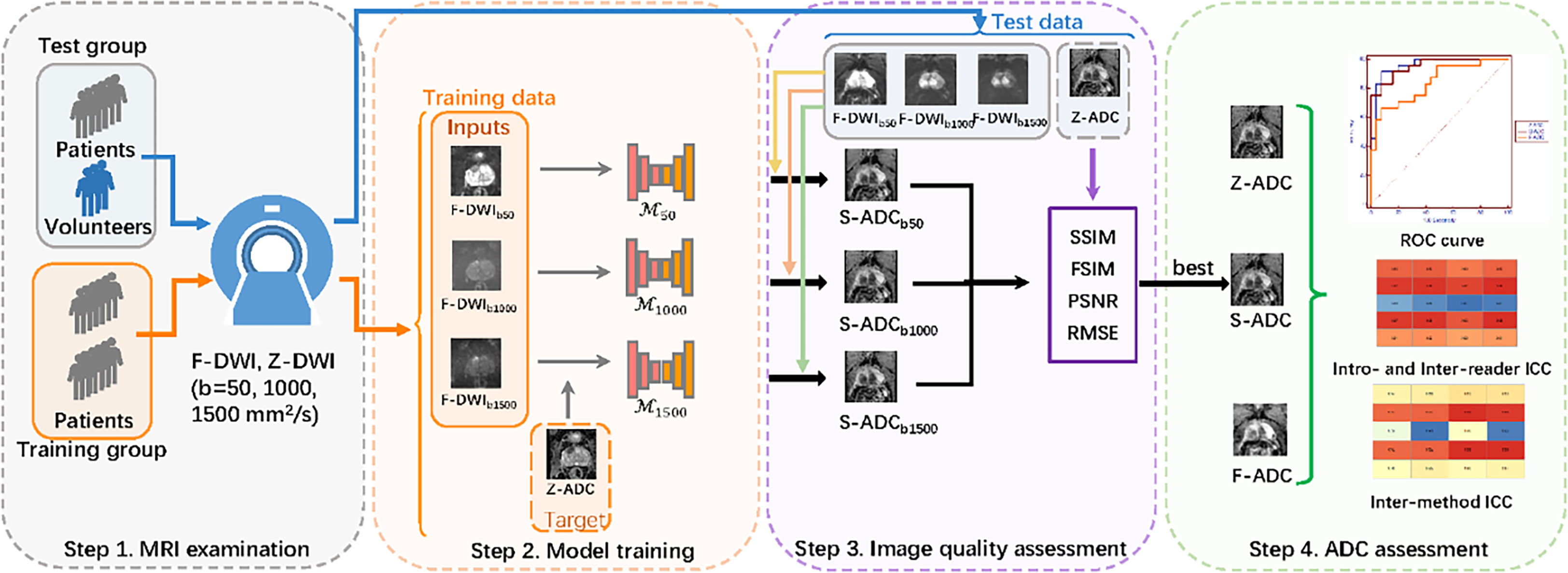
Figure 1 Overall study flow diagram. Step 1: All the patients and healthy volunteers underwent multiparametric magnetic resonance imaging examinations of the prostate, including full field-of-view (FOV) diffusion-weighted imaging (f-DWI) and zoomed FOV diffusion-weighted imaging with b-values of 50, 1,000, and 1,500 s/mm². Step 2: The models that used full f-DWI with different b-values (f-DWI_b50, f-DWI_b1000, and f-DWI_b1500) to synthesize the apparent diffusion coefficient (s-ADC) maps (s-ADC_b50, s-ADC_b1000, and s-ADC_b1500) were trained. Step 3: The image quality of s-ADC_b50, s-ADC_b1000, and s-ADC_b1500 were evaluated using the peak signal-to-noise ratio, root mean square error, structural similarity, and feature similarity. Step 4: An ADC assessment was performed to determine reproducibility, tumor detection, and classification.

MRI Examinations and Datasets

All the patients and volunteers underwent multiparametric MRI examinations of the prostate using a 3T MRI scanner (MAGNETOM Skyra, Siemens Healthcare, Erlangen, Germany) equipped with a phased-array 18-channel body coil and an integrated 32-channel spine coil. Both a transversal single-shot full FOV-EPI DWI (f-DWI) and a prototypic non-parallel transmission zoomed EPI DWI (z-DWI) with b-values of 50, 1,000, and 1,500 s/mm² were performed with the ADC reconstruction maps (f-ADC and z-ADC) using a standard mono-exponential with all the acquired b-values (14). Axial T2-weighted images were obtained from all the participants, and the total examination time was approximately 7 min and 40 s. The detailed scan parameters are shown in Table 1.

TABLE 1

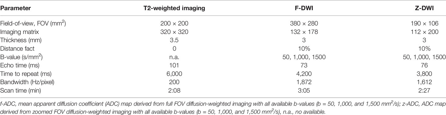
Table 1 The magnetic resonance imaging sequence parameters.

Patient images were randomly divided into two groups (training set: 150 patients, test set #1: 50 patients). The training set was used to build the framework and train different models to synthesize the ADC maps (s-ADCs). Test set #1 was used to test the reproducibility of the s-ADC prostate lesion measurements, along with tumor detection. The images of the healthy volunteers were regarded as test set #2, which was used to test the reproducibility and consistency of the normal prostate tissue s-ADC calculations, including the peripheral zone (PZ) and the transitional zone (TZ).

Data Pre-Processing

Before the model training could occur, image selection, cropping, and registration were performed on f-DWI with b-values of 50, 1,000, and 1,500 s/mm² and the z-ADC images. The first and last slices that did not cover the prostate were removed manually. The images with severe distortion and artifacts were also removed. Ultimately, there were between five and 20 DWI images selected for each person. Finally, there were 2,250 images from each set for the 150 patients in the training set, 750 images from each set for the 50 patients in test set #1, and 145 images from each set for the 10 healthy volunteers in test set #2.

Due to hardware limitations of the graphics cards and the CPU memory, we used only axial slices of the cropped data to train the two-dimensional generation models. The f-DWI data had an original voxel size of 2.13 × 2.13 × 3.3 mm³ and a matrix size of 178 ×132, whereas the z-ADC data had a voxel size of 0.95 × 0.95 × 3.3 mm³ and a matrix size of 112 × 200. The f-DWI data were first resampled to a voxel size of 0.95 × 0.95 × 3.3 mm³ with a matrix size of 360 × 267, and both modalities were cropped at the center to extract the relevant prostate region. The f-DWI data were then aligned to the z-ADC data using the affine transformation implemented by the Advanced Normalization Tools (https://github.com/ANTsX/ANTs). To facilitate the model training, all the two-dimensional axial slices were scaled to a unified resolution of 224 × 224 pixels.

To select a suitable b-value for ADC synthesis, we first used 2,250 paired f-DWI images with b-values of 50 s/mm² and the ground truth z-ADC maps from the training set as inputs and references, respectively, to train our framework-based model M₅₀ to synthesize ADC maps (s-ADC_b50). Similarly, the M₁₀₀₀ and M₁₅₀₀ models based on the f-DWI images with b-values of 1,000 and 1,500 s/mm² were trained to synthesize ADC maps (s-ADC_b1000 and s-ADC_b1500).

Model Training

We have proposed a GAN-based framework to generate realistic z-ADC maps from f-DWI maps (Figure 2).

FIGURE 2

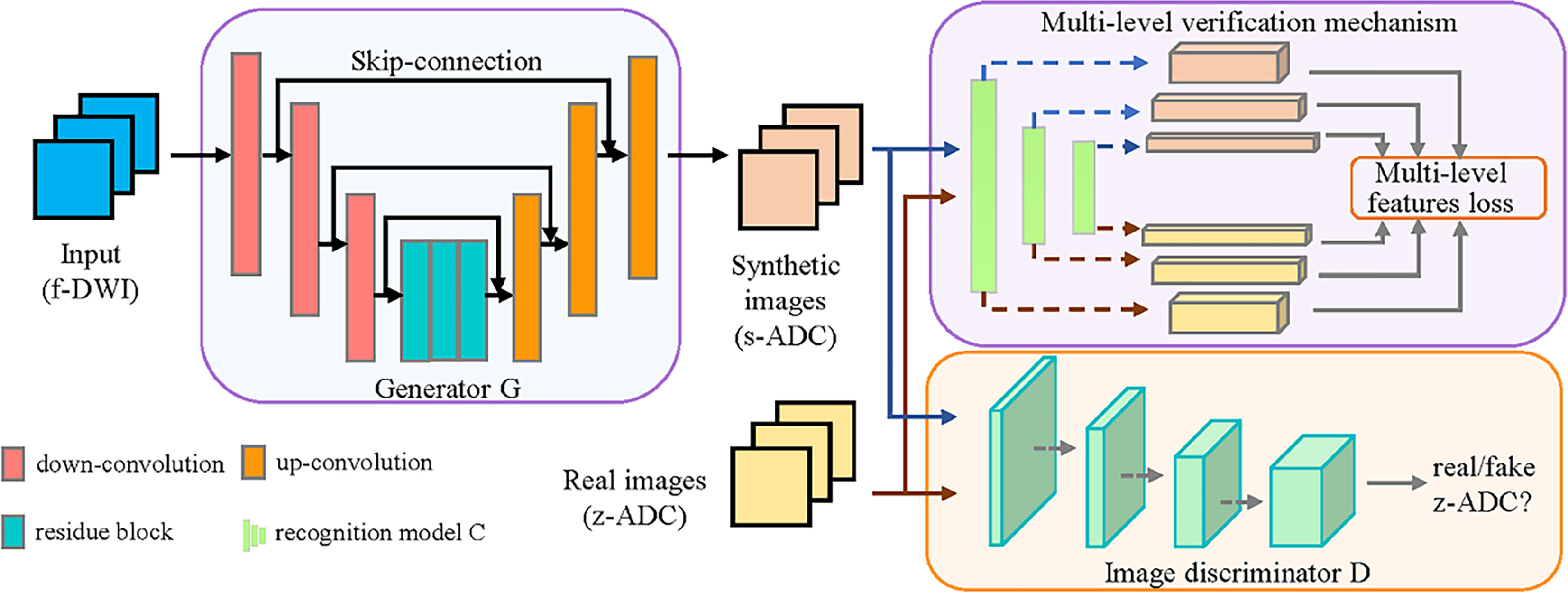
Figure 2 Illustration of our framework. The proposed framework consists of a generator (G), which was constructed using a deep convolution network with skip connections, and an image discriminator (D) constructed using a full convolution network. The G transforms the f-DWI into a synthesized apparent diffusion coefficient (s-ADC) using zoomed field-of-view diffusion-weighted imaging (z-ADC) as a reference. The D takes either s-ADC or z-ADC as the input and determines whether the input is a real z-ADC. In addition, to promote G in an effort to retain better features for diagnosis, we introduced a multi-level verification mechanism, including a pre-trained recognition model (C), to extract the multi-level features from the s-ADC and the z-ADC.

The generator G translates the input image (f-DWI) X into the synthesized ADC (s-ADC) S with a quality similar to the ground truth z-ADC, which is used as reference Y. The discriminator D takes either the S or the Y as input and determines whether the input is a real z-ADC map. Specifically, we used a deep residual network structure with skip connections to construct the generator G and a full convolution network to construct the discriminator D. The adversarial loss of the discriminator D is formulated as follows:

$${ℒ}_D=E_{Y\sim P_Y}[{(D(Y)-1)}^2]+E_{S\sim P_S}[{(D(S))}^2]$$

The adversarial loss of the generator G is formulated as follows:

$${ℒ}_G^{adv}=E_{S\sim P_S}[{(D(S)-1)}^2]$$

Considering that the standard GAN might not adequately preserve the tumors/lesions during image-to-image translation (26), we introduced a multi-level verification (MLV) mechanism, including a pre-trained recognition model C. This mechanism promotes the generator G to better retain the features, which helps in the diagnosis. Using C, the proposed MLV mechanism provides more details about the tumor/lesion features when they are extracted from the input images. G represents the tumor/lesion texture, making it better and more robust against changes in appearance and geometric transformations (27).

We first obtained a recognition model C, which was pre-trained on a VGG-19-based network using the processed images from the patients and healthy volunteers with a benign or malignant label (28). Subsequently, the multiple layers of model C extracted the multi-level features from the fake synthetic ADC map S and the ground truth ADC map. The sum of the mean square errors of the features in each level layer was used as the multi-level feature loss to supervise the generator G.

Inspired by the current work (29) and considering the use of multi-level features, we selected the features in the 0, 1st, 3rd, and 5th level layers. The loss of the multi-level verification mechanism is formulated as follows:

$${ℒ}_G^{mlv}={\Sigma }_{i=0,1,3,5}{\theta }_i·{\left|\right|C^i(S)-C^i(Y)\left|\right|}_2^2$$

where θ_i ∈ (0, 1) denotes the weight parameter for the loss $({ℒ}_{mlf}^i)$ at different levels, and it is optimized in each epoch to cause a faster decrease in the loss of the larger items. The θ_i in the j - th epoch can be computed as follows:

$${\theta }_i^j={\Sigma }_{n=0,1,3,5}\frac{{\left|\right|C_i^{j-1}(S)-C_i^{j-1}(Y)\left|\right|}_2^2}{{\left|\right|C_n^{j-1}(S)-C_n^{j-1}(Y)\left|\right|}_2^2}$$

where $C_i^{j-1}(·)$ denotes the feature of the i - th layer in the (j-1)-th epoch, and $C_n^{j-1}(·)$ indicates the feature of the n - th layer in the (j-1)-th epoch. We initialized θ_i to 1/4. The objective function of generator G is formulated as follows:

$${ℒ}_G={ℒ}_G^{adv}+{\lambda }_1{ℒ}_G^{mlv}$$

with γ₁ set to 10^-1.

Experimental Settings

The generator consists of three convolution layers, followed by five residual blocks and three deconvolution layers. Each convolution or deconvolution layer is followed by an instance-normalization layer and a ReLu activation layer. The discriminator consists of five convolution layers. The learning rate was set to 0.001 for both the generator and the discriminator. The batch size was set to 5, and the epoch was set to 50. The details of the generator and discriminator can be found at https://github.com/huxiaolie/ADC_generation. All the algorithms were implemented using Python 3.6 (https://www.python.org/downloads/release/python-362/) and Pytorch 1.6.0 (https://pytorch.org/get-started/previous-versions/) on an Ubuntu 16.04 system with an NVIDIA TITAN XP GPU.

Image Quality Assessment

The s-ADC sets were synthesized using each model with inputs from the f -DWI images with b-values of 50, 1,000, and 1,500 s/mm² for test set #1 (50 patients) and test set #2 (10 healthy volunteers), and they were compared using peak signal-to-noise ratios (PSNRs), root mean square errors (RMSEs), structural similarities (SSIMs), and feature similarities (FSIMs) (30).

A radiologist with 6 years of experience with prostate MRIs measured the anterior–posterior (AP) and left–right (LR) diameters of each prostate on the ADC set on the slice on which the prostate showed the greatest cross-sectional area. The differences in the measured AP and LR diameters of the prostate relative to the T2-weighted image (T2WI) were computed for f-ADC, z-ADC, and s-ADC, with the best performance from the above-mentioned quantitative evaluation.

ADC Measurement Assessment

For the patient study, two radiologists with 5 and 10 years of experience with prostate MRIs and who were unaware of the clinical, surgical, and histologic findings independently drew a circular region of interest (ROI) with an area of approximately 0.5–0.8 cm² in the center of the lesion, excluding its edges. For the healthy volunteer study, the readers drew circular ROIs with an area of approximately 0.5 cm² in the peripheral and transitional zones on the ADC maps using axial T2-weighted images as the anatomical reference. The mean ADC values for each ROI were recorded.

The ADC sets of all the patients and healthy volunteers were measured twice using Image J (NIH Image, Bethesda, MD) in a different order, with an interval of 2 weeks. The first measurement given by the two readers showed the consistency of the ADC measurements for each ADC set. The second measurement showed the repeatability of the ADC values for each ADC set.

Tumor Detection Assessment

The s-ADC set with the best image quality and ADC measurement assessment among the three s-ADC sets was selected for tumor detection assessments. The selected s-ADC was compared with the f-ADC and z-ADC in terms of the ability to differentiate benign from malignant lesions. The correlation between the ADC values in the different ADC sets and tumor grades was also evaluated.

Statistical Analyses

Analyses of the baseline characteristics between the training group and the test group were conducted. An independent t-test was used to assess normally distributed continuous variables. The Mann–Whitney U-test was used to assess non-normally distributed continuous variables.

To assess differences in the image quality metrics (PSNR, RMSE, SSIM, and FSIM) between any two s-ADC sets, a paired Student’s t-test was applied. The intraclass correlation coefficient (ICC) was used to assess the inter-and intra-reader repeatability of the ADC measurements for each tissue (malignant lesion, benign lesion, peripheral zone, and transitional zone) in each ADC set (f-ADC, z-ADC, and s-ADC). The ICC was also used to evaluate the inter-method reliability of the ADC values for each tissue between the synthesized image (s-ADC) and the reference image (z-ADC). A receiver operating characteristic (ROC) curve analysis was performed to assess the ability to discriminate between benign and malignant prostate lesions based on the ADC values. The differences in the area under the curve (AUC) values were tested using DeLong tests. The statistical analyses were performed using MedCalc software. Two-tailed tests were used to calculate all the P-values. Statistical significance was set at P <0.05.

Results

Demographic Characteristics

The patient characteristics are summarized in Table 2. There were no significant differences in the mean ages between the patients with and without PCa (P = 0.557). The mean prostate-specific antigen (PSA) level was significantly higher in patients with PCa compared to those without PCa (P < 0.001).

TABLE 2

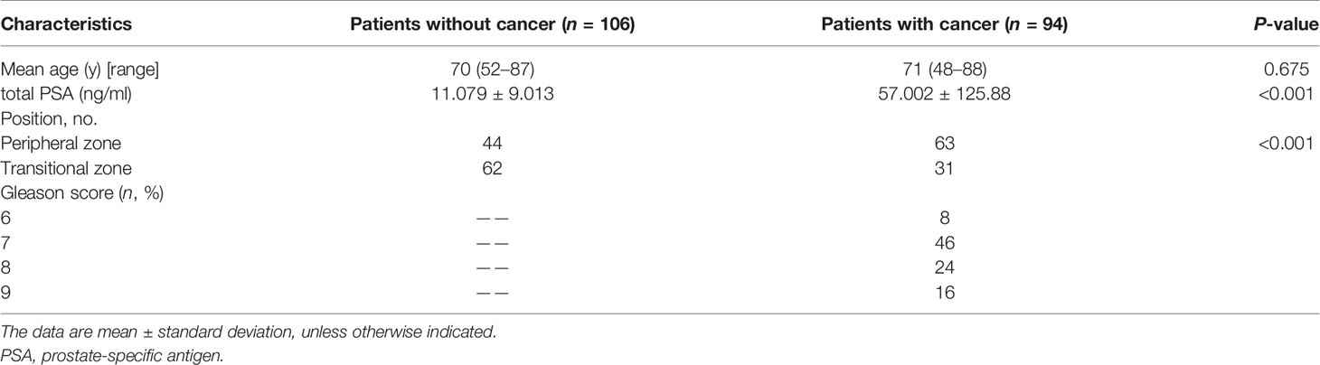
Table 2 The clinical characteristics of the patient cohort.

There were no significant differences in mean ages and mean PSA between the training set and test set #1 (mean ages: 68 ± 10 vs. 68 ± 12 years, P = 0.974; PSA: 29.872 ± 69.461 vs. 39.296 ± 92.604, P = 0.154). The mean age of test set #2 (healthy volunteers, 24 ± 3 years) is significantly lower than that of the training set and test set #1 (P < 0.001).

Image Quality Assessment

Visual comparisons of the s-ADC values generated with different b-value inputs are shown in Figure 3. We observed that the s-ADC_b50 displayed blurred images of the prostate, bladder, rectum, pelvic floor muscles, and pubic symphysis in both the patients and the volunteers. Compared with s-ADC_b50, s-ADC_b1000 and s-ADC_b1500 could delineate normal tissues and lesions more clearly and sharply, which was in line with the ground truth. According to the magnified images of the local tissue structures, s-ADC_b1000 provided more details than s-ADC_b1500 with reference to z-ADC.

FIGURE 3

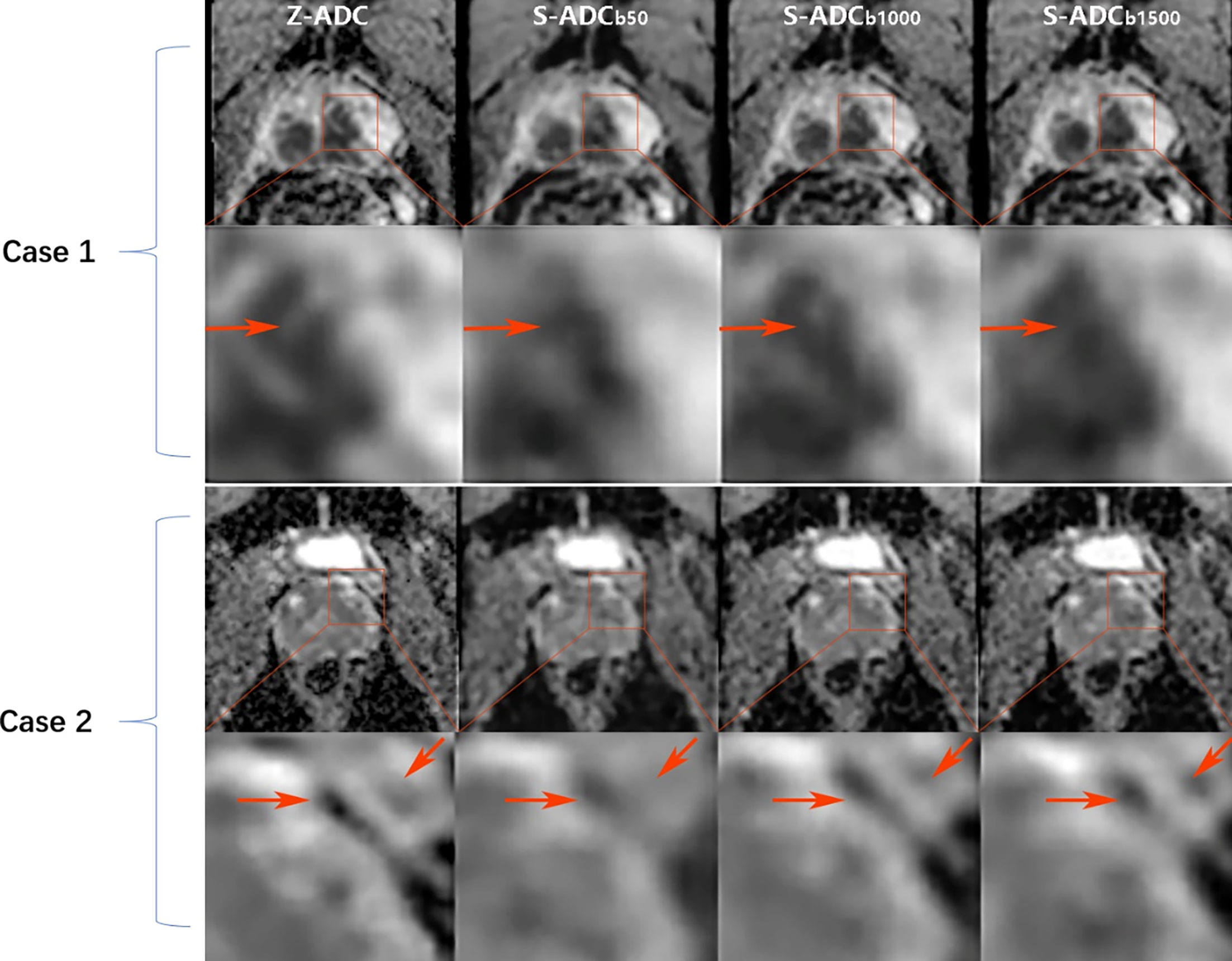
Figure 3 Comparison of the synthesized apparent diffusion coefficient (s-ADC) maps. Case 1: An 82-year-old man with prostate cancer from test set 1 who had an initial prostate-specific antigen level of 13.04 ng/ml. Case 2: A 27-year-old healthy man from test set 2. For these two cases, both the s-ADC_b1000 and s-ADC_b1500 performed well in displaying the prostate, pelvic floor muscles, pubic symphysis, and the entire cancer lesion. However, the s-ADC_b50 images of these structures are fuzzy. According to the local enlargement of the images (the images in the second and fourth lines), the s-ADC_b1000 is more similar to the z-ADC than to the s-ADC_b1500, and it retains more details of the z-ADC (shown as red arrows).

As shown in the violin plots (Figure 4), s-ADC_b1000 performed better than the other two s-ADC sets in terms of the distribution, median, and inter-quartile ranges of the RMSE, SSIM, FSIM, and PSNR scores. The mean RMSE scores of s-ADC_b50, s-ADC_b1000, and s-ADC_b1500 were 4.1 × 10^-3, 2.5 × 10^-3, and 3.1 × 10^-3, respectively. The mean PSNR scores of s-ADC_b50, s-ADC_b1000, and s-ADC_b1500 were 48.0, 53.4, and 51.0, respectively. The mean SSIM scores of s-ADC_b50, s-ADC_b1000, and s-ADC_b1500 were 0.972, 0.986, and 0.982, respectively. The mean FSIM scores of s-ADC_b50. s-ADC_b1000, and s-ADC_b1500 were 0.604, 0.728, and 0.690, respectively. s-ADC_b1000 had a significantly lower RMSE score and higher PSNR, SSIM, and FSIM scores than s-ADC_b50 and s-ADC_b1500 (all P < 0.05).

FIGURE 4

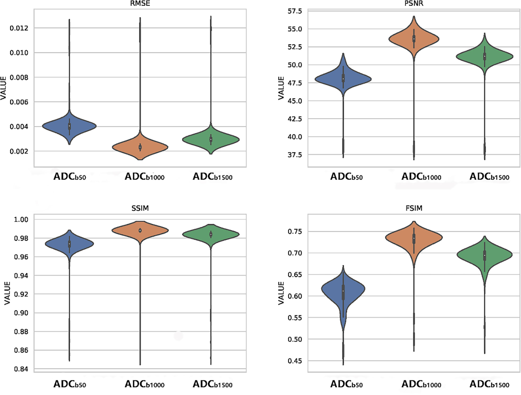
Figure 4 Violin plots of the quantitative metric distributions of the s-ADC sets.

To evaluate the distortion in the ADC maps, the differences in the AP and LR diameters of the prostate relative to T2WI were both significantly lower for s-ADC (AP, 2.734; LR, 3.204) and z-ADC (AP, 2.755; LR, 3.073) than for f-DWI (AP, 5.916; LR, 5.053) (all P < 0.001).

ADC Measurement Assessment

The measurements of all the ADC sets (f-ADC, z-ADC, s-ADC_b50, ADC_b1000, and s-ADC_b1500) on various tissues from both readers are presented in Table 3. For all the ADC sets, the ADC values of the TZ are significantly lower than those of the PZ, while the ADC values of the malignant lesions are significantly lower than those of the benign lesions (all P < 0.05).

TABLE 3

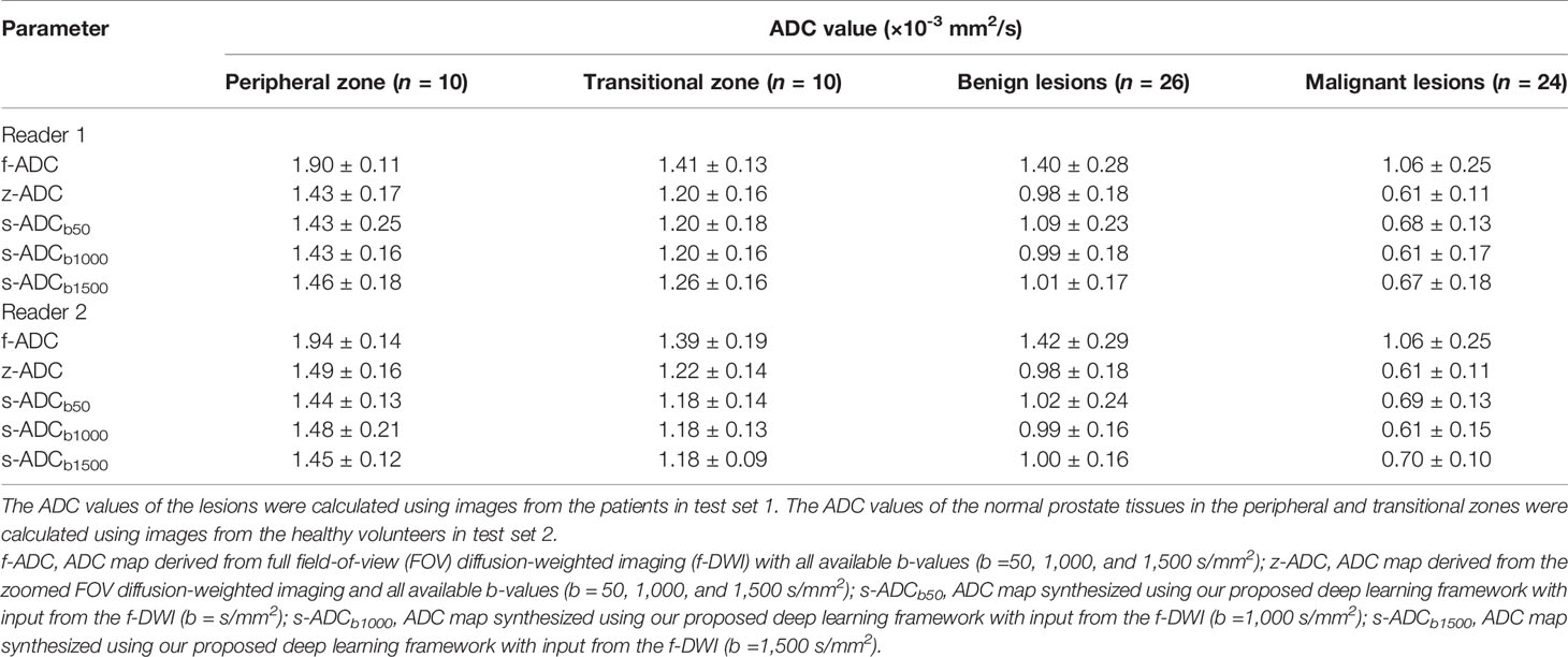
Table 3 The mean apparent diffusion coefficient (ADC) values (×10^-3 mm²/s) of the different ADC sets.

Figure 5 presents the results of the intra-reader reproducibility (Figures 5A, B) and inter-reader consistency (Figure 5C) analyses for each ADC set calculation. Both readers reported that the reproducibility of the ADC measurements for f-ADC, z-ADC, s-ADCb1000, and s-ADCb1500 was excellent for all the tissues, while the reliability of the ADC measurements for s-ADC_b50 was good. The inter-reader consistency of all the ADC set measurements was excellent for all the tissues. Table 4 shows the consistency of the ADC values between the z-ADC and s-ADC sets. The consistency of the ADC values in the transitional zone between z-DWI and s-DWI_b50 was good, and the consistency of the ADC values between z-ADC and s-ADC_b50 for the remaining tissues was excellent. For the s-ADC_b1000 and s-ADC_b1500 values, the consistency of the ADC values for z-ADC for all the tissues was excellent.

FIGURE 5

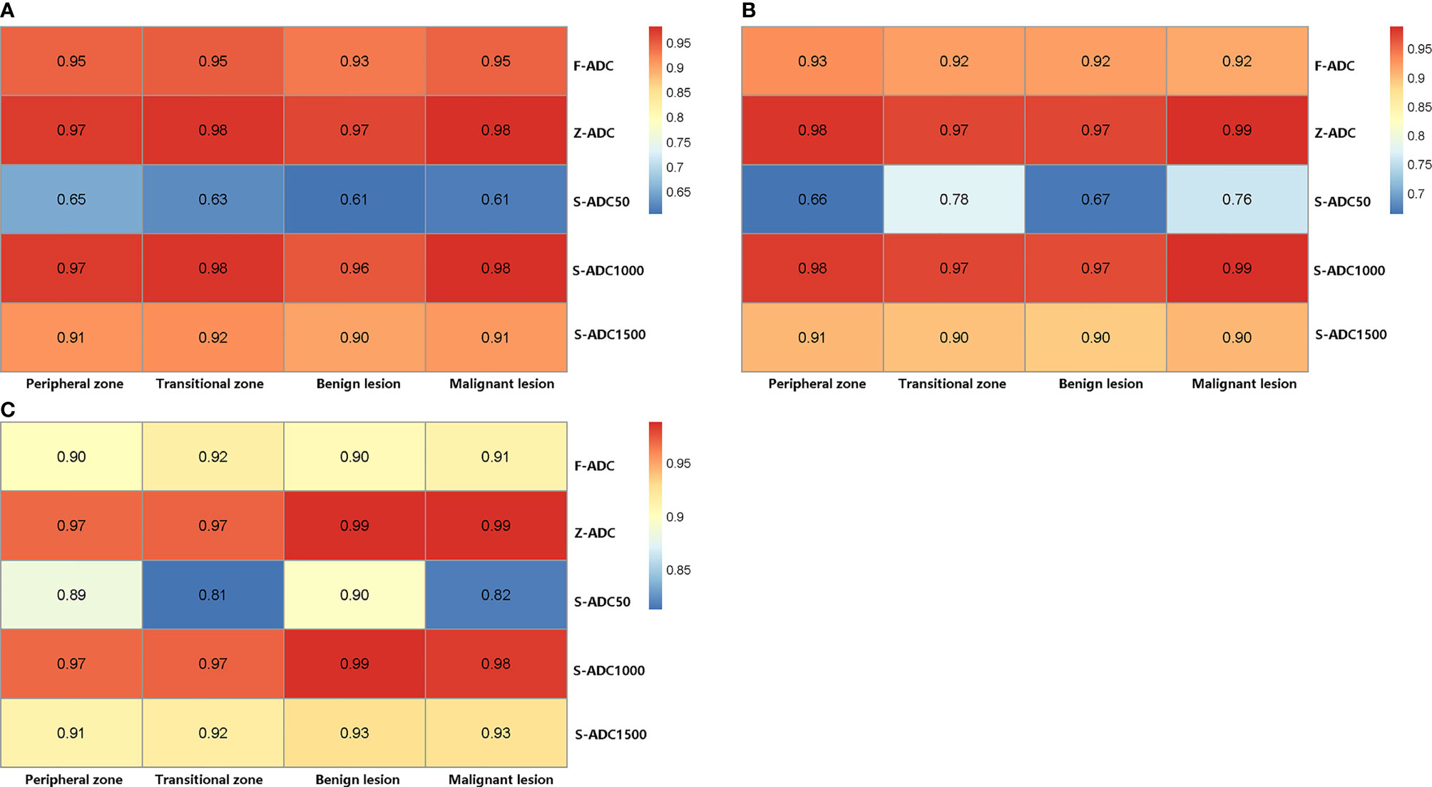
Figure 5 The reproducibility of the apparent diffusion coefficient (ADC) measurements as evaluated by the intraclass correlation coefficient. (A) The ADC measurement repeatability of reader 1 and (B) reader 2, and (C) the consistency of the ADC measurements between readers 1 and 2.

TABLE 4

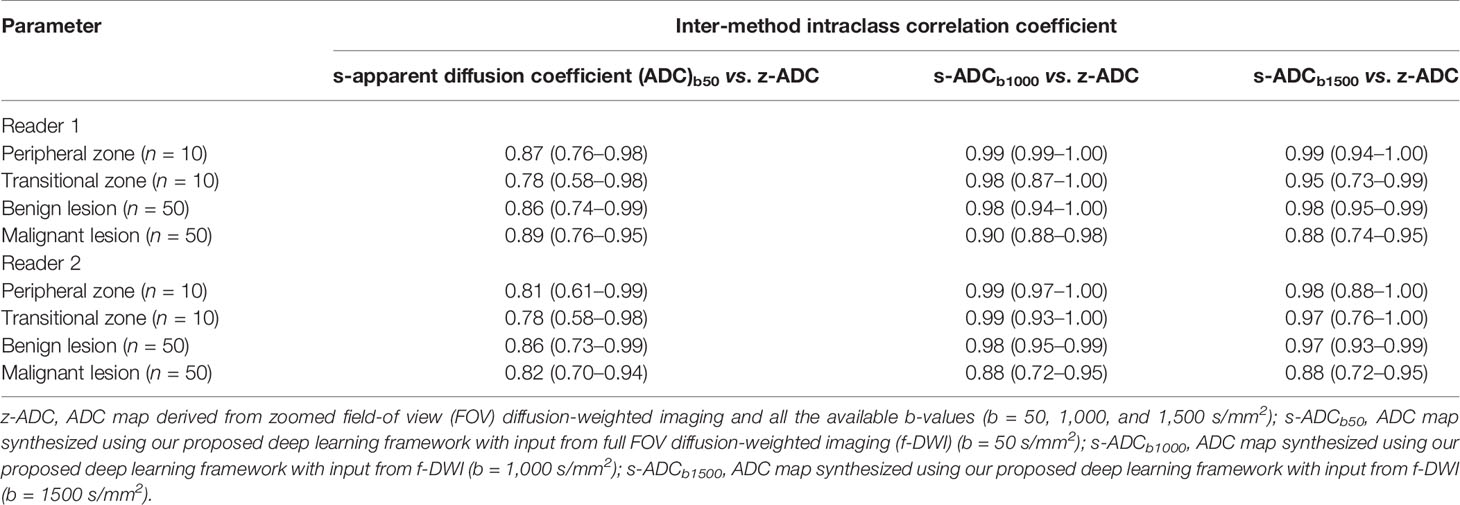
Table 4 Comparison between the inter-method intraclass correlation coefficients from the z-DWI and s-DWI sets.

Tumor Detection Assessment

Among the three s-ADC sets, s-ADC_b1000 performed the best in the image quality assessment and ADC evaluation. Therefore, it was selected for further comparisons with f-ADC and z-ADC in terms of tumor detection and classification (Figure 6). The ADC values for patients with malignant lesions and those with benign lesions measured by the two readers were used to compute the ROC curves (Figure 7). The comparisons of AUCs for both readers based on the f-ADC, z-ADC, and s-ADC sets are summarized in Table 5. Both the z-ADC and s-ADC sets showed significantly better predictive capabilities than the f-ADC set (P ≤ 0.027). The differences in AUCs between s-ADC and z-ADC were not statistically significant (reader 1: z = 0.134, P = 0.893; reader 2: z = 0.094, P = 0.925).

FIGURE 6

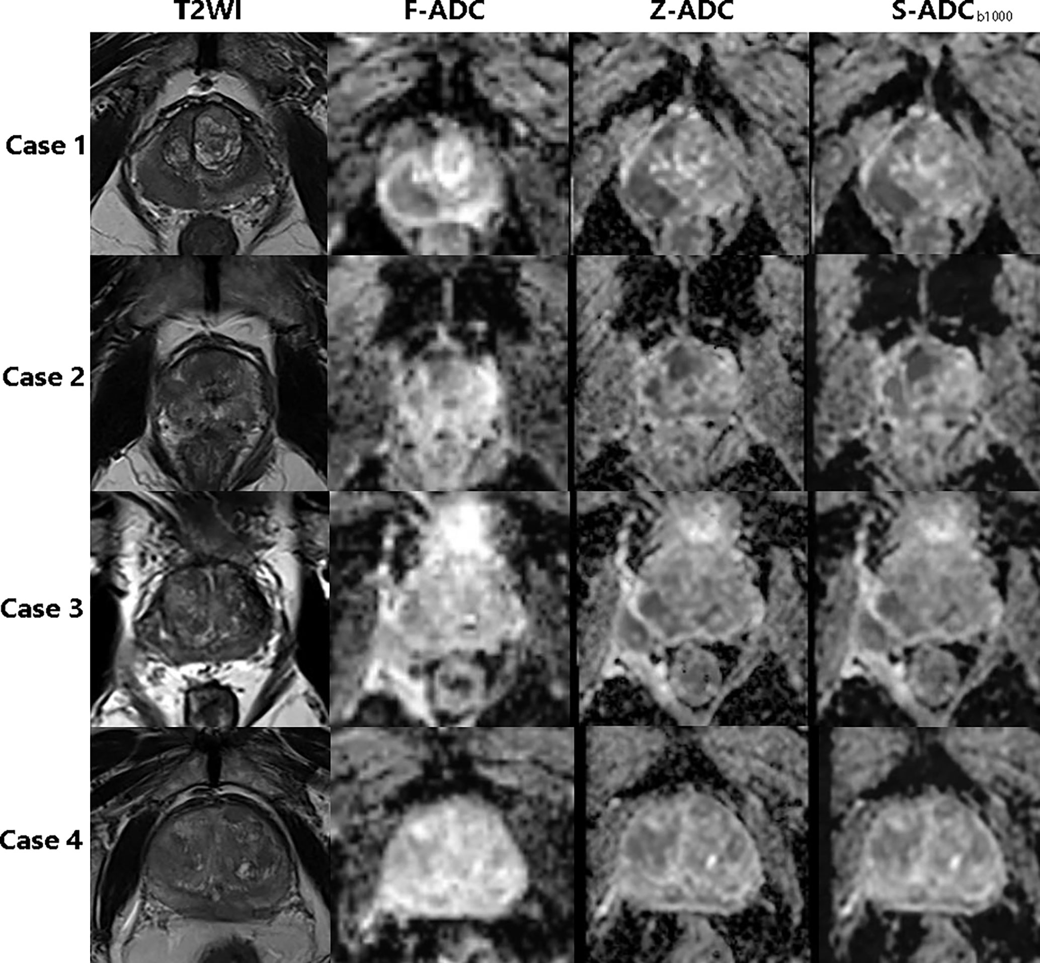
Figure 6 The T2-weighted image, f-ADC, z-ADC, and s-ADC_b1000 of four different patients. Case 1: An 85-year-old man with prostate cancer in the right peripheral zone and an initial prostate-specific antigen level of 0.157 ng/ml. Case 2: An 85-year-old man with prostate cancer in the central zone and an initial prostate-specific antigen level of 21.44 ng/ml. Case 3: A 67-year-old man with an inflammatory nodule in the right peripheral zone and an initial prostate-specific antigen level of 14.37 ng/ml. Case 4: A 77-year-old man with prostate cancer in the central zone and an initial prostate-specific antigen level of 56.62 ng/ml.

FIGURE 7

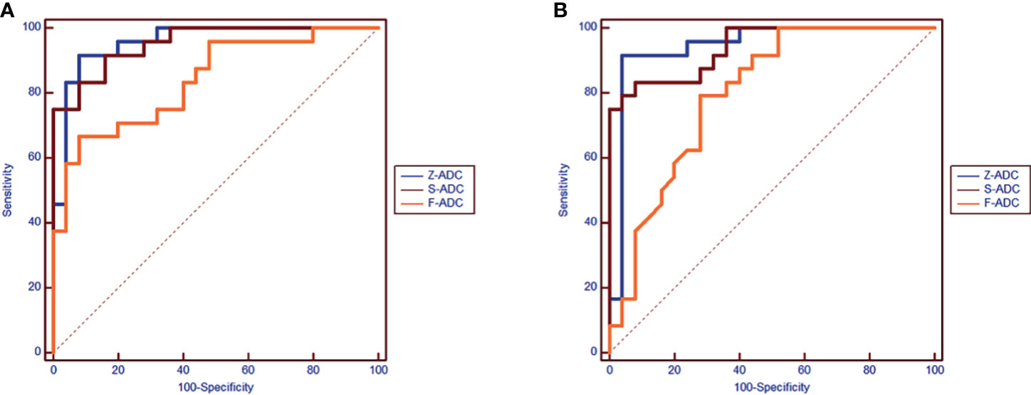
Figure 7 The receiver operating characteristic comparison of the diagnostic accuracy of the f-ADC, z-ADC, and s-ADCb1000 sets (A: reader 1, B: reader 2).

TABLE 5

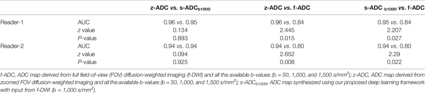
Table 5 The comparison of areas under the curve (AUCs) based on the f-apparent diffusion coefficient (ADC), z-ADC, and s-ADC sets for both readers.

Discussion

The main contribution of our study to the literature is the proposed GAN-based ADC synthesis method that can be used to generate s-ADC maps using single b-value DWIs with better image quality and stronger ADC calculation accuracy and reproducibility than a full FOV ADC, but without dependence on software, hardware, and additional scanning time that zoomed FOV ADC technology requires. A shorter scan time will lead to better patient comfort and fewer motion artifacts due to involuntary or autonomous motions. The high reproducibility and accuracy of the ADC calculations may effectively reduce the risk of delayed treatment or unnecessary overtreatment due to the misdiagnoses of benign and malignant lesions. Therefore, the GAN-based ADC synthesis method can increase the clinical benefits to patients, reduce treatment times, and lower the costs incurred by patients and hospitals.

In previous studies (31–33), GANs have been used successfully for image-to-image transformations, such as in generating MRI or PET images using CT images or synthesizing CT images from MRI images, and they have performed well in terms of the traditional pixel-wise metrics. However, GAN-generated images do not have a physical meaning, and they can often lead to spurious images (21). As a result, it is difficult for GANs and their extensions to win the trust of clinicians. Therefore, we not only compared traditional pixel-wise metrics, including the RMSE, SSIM, FSIM, and PSNR scores, between the s-ADC sets and reference images, but we also compared the s-ADC and ADC values generated by traditional methods to evaluate the clinical value of GAN-generated images.

In the present study, we evaluated s-ADC maps that were based on DWI inputs with different b-values and found that the choice of b-values influenced the s-ADC values. Based on a subjective visual evaluation, the s-ADC_b1000 maps delineated normal tissues and lesions more clearly than the s-ADC_b50 maps, and they provided more details for targeted images than the s-ADC_b1500 set. The quantitative evaluation results are also consistent with the visual evaluation results. Among the three s-ADC sets, the s-ADC_b1000 set achieved a lower RMSE score and higher SSIM, FSIM, and PSNR scores than the s-ADC_b50 and s-ADC_b1500 sets, indicating that the s-ADC_b1000 set is more similar to the realistic z-ADC in terms of noise distribution, image structure, and features. Additionally, the s-ADC_b1000 set showed better intra-reader repeatability and inter-reader consistency than the s-ADC_b50 and s-ADC_b1500 sets. Moreover, the s-ADC_b1000 set showed the best ADC value inter-method consistency with the z-ADC set, suggesting that a DWI with a b-value of 1,000 s/mm² might be more suitable for synthesizing ADC maps than one with a b-value of 50 or 1,500 s/mm². The similarity between the target image z-DWI and s-DWI strongly depends on how much useful information the input f-DWI can provide to the generator for the extraction of meaningful features to begin the mapping between f-DWI and z-ADC. Low-b-value DWIs suffer from T2 shine-through or black-through effects, whereas high-b-value DWIs might be affected by diffusion kurtosis effects (34). These effects have a negative influence on image quality and lesion information, causing a relatively lower similarity between the s-ADC_b50 and s-ADC_b1500 sets and the z-ADC set compared to the s-ADC_b1000 set (3).

In our study, both the z-ADC and s-ADC sets showed less distortion and better reproducibility of the quantitative ADC values for all the evaluated tissues; they also showed better tumor detection and classification capacity than the f-ADC sets. The ADC values are generated for most of the current clinical implementations by calculating the signal intensity decay using two or more DWI sets with different b-values (1–5, 9–11, 13, 14). The reproducibility and accuracy of the calculated ADC values are affected by the choice of b-values (3, 4, 34) and the DWI image quality (14). The application of a significant number of b-values improves the reproducibility and accuracy of the calculated ADC values, although it also increases the scanning time (3, 35). In contrast to traditional ADC calculation methods, our proposed method takes advantage of the ability of GAN to simulate data distribution and synthesize ADC maps that are highly similar to real zoomed FOV ADC maps that use a full FOV DWI with a single b-value. Considering the excellent image quality consistency and similar tumor detection and classification abilities between the s-ADC and z-ADC maps, we believe that the deep learning algorithm might be a feasible method for generating ADC maps as an alternative to z-ADC maps without requiring a strong dependence on software, hardware, and additional scan time (36).

Our study has several limitations. First, the s-ADC_b1000 set showed the best image quality among the s-ADC sets; however, it remains unknown whether a DWI set with a b-value of 1,000 s/mm² is the most appropriate for ADC map synthesis. In future studies, s-ADC sets generated using DWI sets with more potential b-values should be compared. Second, as ADC values vary across vendors, the generalizability of our model across MRI scanners from different vendors requires multi-center verification.

In conclusion, the GAN-based ADC synthesis method can generate s-ADC maps using a single b-value DWI with good image quality and high reproducibility and ADC calculation accuracy.

Data Availability Statement

The original contributions presented in the study are included in the article/supplementary material. Further inquiries can be directed to the corresponding author.

Ethics Statement

The studies involving human participants were reviewed and approved by The ethics committee of Shanghai Jiao Tong University Affiliated Sixth People’s Hospital. The patients/participants provided their written informed consent to participate in this study. Written informed consent was obtained from the individual(s) for the publication of any potentially identifiable images or data included in this article.

Author Contributions

JZ is the guarantor of the integrity of the entire study (study concepts/study design, data acquisition, and data analysis/interpretation). LH participated in statistical analysis, manuscript drafting and manuscript revision for important intellectual content. LH and JZ edited the manuscript. LH and DZ participated in literature research. LH, DZ, YX, and LW participated in clinical studies. All authors contributed to the article and approved the submitted version.

Funding

This study was funded by the National Natural Science Foundation of China (nos. 81901845 and 81671791), the Science Foundation of Shanghai Jiao Tong University Affiliated Sixth People’s Hospital (no. 201818), and the Shanghai Key Discipline of Medical Imaging (no. 2017ZZ02005).

Conflict of Interest

CF was employed by Siemens Shenzhen Magnetic Resonance, Ltd. TB was employed by MR Application Predevelopment, Siemens Healthcare GmbH, Erlangen, Germany.

The remaining authors declare that the research was conducted in the absence of any commercial or financial relationships that could be construed as a potential conflict of interest.

Publisher’s Note

All claims expressed in this article are solely those of the authors and do not necessarily represent those of their affiliated organizations, or those of the publisher, the editors and the reviewers. Any product that may be evaluated in this article, or claim that may be made by its manufacturer, is not guaranteed or endorsed by the publisher.

References

1. Turkbey B, Shah VP, Pang Y, Bernardo M, Xu S, Kruecker J, et al. Is Apparent Diffusion Coefficient Associated With Clinical Risk Scores for Prostate Cancers That are Visible on 3-T MR Images? Radiology (2011) 258(2):488–95. doi: 10.1148/radiol.10100667

PubMed Abstract | CrossRef Full Text | Google Scholar

2. Hambrock T, Somford DM, Huisman HJ, van Oort IM, Witjes JA, Hulsbergen-van de Kaa CA, et al. Relationship Between Apparent Diffusion Coefficients at 3.0-T MR Imaging and Gleason Grade in Peripheral Zone Prostate Cancer. Radiology (2011) 259(2):453–61. doi: 10.1148/radiol.11091409

PubMed Abstract | CrossRef Full Text | Google Scholar

3. Turkbey B, Rosenkrantz AB, Haider MA, Padhani AR, Villeirs G, Macura KJ, et al. Prostate Imaging Reporting and Data System Version 2.1: 2019 Update of Prostate Imaging Reporting and Data System Version 2. Eur Urol (2019) 76(3):340–51. doi: 10.1016/j.eururo.2019.02.033

PubMed Abstract | CrossRef Full Text | Google Scholar

4. Surov A, Meyer HJ, Wienke A. Correlations Between Apparent Diffusion Coefficient and Gleason Score in Prostate Cancer: A Systematic Review. Eur Urol Oncol (2020) 3(4):489–97. doi: 10.1016/j.euo.2018.12.006

PubMed Abstract | CrossRef Full Text | Google Scholar

5. Bai K, Sun Y, Li W, Zhang L. Apparent Diffusion Coefficient in Extraprostatic Extension of Prostate Cancer: A Systematic Review and Diagnostic Meta-Analysis. Cancer Manag Res (2019) 11:3125–37. doi: 10.2147/CMAR.S191738

PubMed Abstract | CrossRef Full Text | Google Scholar

6. Nguyen TB, Ushinsky A, Yang A, Nguyentat M, Fardin S, Uchio E, et al. Utility of Quantitative Apparent Diffusion Coefficient Measurements and Normalized Apparent Diffusion Coefficient Ratios in the Diagnosis of Clinically Significant Peripheral Zone Prostate Cancer. Br J Radiol (2018) 91(1088):20180091. doi: 10.1259/bjr.20180091

PubMed Abstract | CrossRef Full Text | Google Scholar

7. Kato S, Kamijima S, Inaoka T, Kamiya N, Sasai D, Terada H, et al. Quantitative Evaluation of the Relative Apparent Diffusion Coefficient Values on Multiparametric Magnetic Resonance Imaging to Predict Higher Gleason Score Prostate Cancer. Scand J Urol (2018) 52(3):180–5. doi: 10.1080/21681805.2018.1481143

PubMed Abstract | CrossRef Full Text | Google Scholar

8. Nougaret S, Robertson N, Golia Pernicka J, Molinari N, Hötker AM, Ehdaie B, et al. The Performance of PI-RADSv2 and Quantitative Apparent Diffusion Coefficient for Predicting Confirmatory Prostate Biopsy Findings in Patients Considered for Active Surveillance of Prostate Cancer. Abdom Radiol (NY) (2017) 42(7):1968–74. doi: 10.1007/s00261-017-1086-7

PubMed Abstract | CrossRef Full Text | Google Scholar

9. Gupta RT, Kauffman CR, Garcia-Reyes K, Palmeri ML, Madden JF, Polascik TJ, et al. Apparent Diffusion Coefficient Values of the Benign Central Zone of the Prostate: Comparison With Low- and High-Grade Prostate Cancer. AJR Am J Roentgenol (2015) 205(2):331–6. doi: 10.2214/AJR.14.14221

PubMed Abstract | CrossRef Full Text | Google Scholar

10. Boesen L, Chabanova E, Løgager V, Balslev I, Thomsen HS. Apparent Diffusion Coefficient Ratio Correlates Significantly With Prostate Cancer Gleason Score at Final Pathology. J Magn Reson Imaging (2015) 42(2):446–53. doi: 10.1002/jmri.24801

PubMed Abstract | CrossRef Full Text | Google Scholar

11. Babourina-Brooks B, Cowin GJ, Wang D. Diffusion-Weighted Imaging in the Prostate: An Apparent Diffusion Coefficient Comparison of Half-Fourier Acquisition Single-Shot Turbo Spin-Echo and Echo Planar Imaging. Magn Reson Imaging (2012) 30(2):189–94. doi: 10.1016/j.mri.2011.09.024

PubMed Abstract | CrossRef Full Text | Google Scholar

12. Nketiah G, Selnaes KM, Sandsmark E, Teruel JR, Krüger-Stokke B, Bertilsson H, et al. Geometric Distortion Correction in Prostate Diffusion-Weighted MRI and its Effect on Quantitative Apparent Diffusion Coefficient Analysis. Magn Reson Med (2018) 79(5):2524–32. doi: 10.1002/mrm.26899

PubMed Abstract | CrossRef Full Text | Google Scholar

13. Mazaheri Y, Vargas HA, Nyman G, Shukla-Dave A, Akin O, Hricak H. Diffusion-Weighted MRI of the Prostate at 3.0 T: Comparison of Endorectal Coil (ERC) MRI and Phased-Array Coil (PAC) MRI-The Impact of SNR on ADC Measurement. Eur J Radiol (2013) 82(10):e515–20. doi: 10.1016/j.ejrad.2013.04.041

PubMed Abstract | CrossRef Full Text | Google Scholar

14. Gibbs P, Pickles MD, Turnbull LW. Repeatability of Echo-Planar-Based Diffusion Measurements of the Human Prostate at 3 T. Magn Reson Imaging (2007) 25(10):1423–9. doi: 10.1016/j.mri.2007.03.030

PubMed Abstract | CrossRef Full Text | Google Scholar

15. Henkelman RM. Measurement of Signal Intensities in the Presence of Noise in MR Images. Med Phys (1985) 12(2):232–33. doi: 10.1118/1.595711

PubMed Abstract | CrossRef Full Text | Google Scholar

16. Gudbjartsson H, Patz S. The Rician Distribution of Noisy MRI Data. Magn Reson Med (1995) 34(6):910–14. doi: 10.1002/mrm.1910340618

PubMed Abstract | CrossRef Full Text | Google Scholar

17. Riffel P, Michaely HJ, Morelli JN, Pfeuffer J, Attenberger UI, Schoenberg SO, et al. Zoomed EPI-DWI of the Pancreas Using Two-Dimensional Spatially Selective Radiofrequency Excitation Pulses. PloS One (2014) 9(3):e89468. doi: 10.1371/journal.pone.0089468

PubMed Abstract | CrossRef Full Text | Google Scholar

18. Rosenkrantz AB, Chandarana H, Pfeuffer J, Triolo MJ, Shaikh MB, Mossa DJ, et al. Zoomed Echo-Planar Imaging Using Parallel Transmission: Impact on Image Quality of Diffusion-Weighted Imaging of the Prostate at 3T. Abdom Imaging (2015) 40(1):120–26. doi: 10.1007/s00261-014-0181-2

PubMed Abstract | CrossRef Full Text | Google Scholar

19. Thierfelder KM, Scherr MK, Notohamiprodjo M, Weiß J, Dietrich O, Mueller-Lisse UG, et al. Diffusion-Weighted MRI of the Prostate: Advantages of Zoomed EPI With Parallel-Transmit-Accelerated 2D-Selective Excitation Imaging. Eur Radiol (2014) 24(12):3233–41. doi: 10.1007/s00330-014-3347-y

PubMed Abstract | CrossRef Full Text | Google Scholar

20. Goodfellow I, Pouget-Abadie J, Mirza M, Xu B, Warde-Farley D, Ozair S, et al. Generative Adversarial Nets. In: Advances in Neural Information Processing Systems. The MIT Press (2014)p. 2672–80.

Google Scholar

21. Armanious K, Jiang C, Fischer M, Kustner T, Hepp T, Nikolaou K, et al. MedGAN: Medical Image Translation Using GANs. Comput Med Imaging Graph (2020) 79:101684. doi: 10.1016/j.compmedimag.2019.101684

PubMed Abstract | CrossRef Full Text | Google Scholar

22. Wolterink JM, Leiner T, Viergever MA, Isgum I. Generative Adversarial Networks for Noise Reduction in Low-Dose CT. IEEE Trans Med Imaging (2017) 36(12):2536–45. doi: 10.1109/TMI.2017.2708987

PubMed Abstract | CrossRef Full Text | Google Scholar

23. Kim KH, Do WJ, Park SH. Improving Resolution of MR Images With an Adversarial Network Incorporating Images With Different Contrast. Med Phys (2018) 45(7):3120–31. doi: 10.1002/mp.12945

PubMed Abstract | CrossRef Full Text | Google Scholar

24. Wang J, Zhao Y, Noble JH, Dawant BM. Conditional Generative Adversarial Networks for Metal Artifact Reduction in CT Images of the Ear. Med Image Comput Dawna Assist Interv (2018) 11070:3–11. doi: 10.1007/978-3-030-00928-1_1

CrossRef Full Text | Google Scholar

25. Johnson PM, Drangova M. Conditional Generative Adversarial Network for 3D Rigid-Body Motion Correction in MRI. Magn Reson Med (2019) 82(3):901–10. doi: 10.1002/mrm.27772

PubMed Abstract | CrossRef Full Text | Google Scholar

26. Cohen JP, Luck M, Honari S. (2018). Distribution Matching Losses can Hallucinate Features in Medical Image Translation, in: International Conference on Medical Image Computing and Computer-Assisted Intervention, Medical Image Computing and Computer Assisted Intervention – MICCAI 2018, Lecture Notes in Computer Science, pp. 529–36.

Google Scholar

27. Xu H, Huang C, Huang X, Xu C, Huang M. Combining Convolutional Neural Network Markov Random Field Semantic Image Retrieval. Adv Multimedia (2018) 2018:1–11.

Google Scholar

28. Simonyan K, Zisserman A. Very Deep Convolutional Networks for Large-Scale Image Recognition. The 3rd International Conference on Learning Representations (2014).

Google Scholar

29. Chen C, Liu W, Tan X, Wong KK. Semi-Supervised Learning for Face Sketch Synthesis in the Wild. In: Jawahar C, Li H, Mori G, Schindler K, editors. Computer Vision – ACCV 2018. Lecture Notes in Computer Science, vol. 11361. Cham: Springer (2018). doi: 10.1007/978-3-030-20887-5_14

CrossRef Full Text | Google Scholar

30. Zhou F, Yao R, Liu B, Qiu G. Visual Quality Assessment for Super-Resolved Images: Database and Method. IEEE Trans Image Process (2019) 28(7):3528–41. doi: 10.1109/TIP.2019.2898638

PubMed Abstract | CrossRef Full Text | Google Scholar

31. Jin CB, Kim H, Liu M, Jung W, Joo S, Park E, et al. Deep CT to MR Synthesis Using Paired and Unpaired Data. Sensors (Basel) (2019) 19(10):2361. doi: 10.3390/s19102361

CrossRef Full Text | Google Scholar

32. Nie D, Trullo R, Lian J, Petitjean C, Ruan S, Wang Q, et al. Medical Image Synthesis With Context-Aware Generative Adversarial Networks. Med Image Comput Jinn Assist Interv (2017) 10435:417–25. doi: 10.1007/978-3-319-66179-7_48

CrossRef Full Text | Google Scholar

33. Bentaieb A, Hamarneh GJI. ToMI. Adversarial Stain Transf Histopathol Image Anal (2017) PP(99):1–1.

Google Scholar

34. Peng Y, Jiang Y, Antic T, Sethi I, Schmid-Tannwald C, Eggener S, et al. Apparent Diffusion Coefficient for Prostate Cancer Imaging: Impact of B Values. AJR Am J Roentgenol (2014) 202(3):W247–53. doi: 10.2214/AJR.13.10917

PubMed Abstract | CrossRef Full Text | Google Scholar

35. Park SY, Kim CK, Park BK, Kwon GY. Comparison of Apparent Diffusion Coefficient Calculation Between Two-Point and Multipoint B Value Analyses in Prostate Cancer and Benign Prostate Tissue at 3 T: Preliminary Experience. AJR Am J Roentgenol (2014) 203(3):W287–94. doi: 10.2214/AJR.13.11818

PubMed Abstract | CrossRef Full Text | Google Scholar

36. Hu L, Zhou DW, Fu CX, Benkert T, Jiang CY, Li RT, et al. Advanced Zoomed Diffusion-Weighted Imaging vs. Full-Field-of-View Diffusion-Weighted Imaging in Prostate Cancer Detection: A Radiomic Features Study. Eur Radiol (2021) 31(3):1760–9. doi: 10.1007/s00330-020-07227-4

PubMed Abstract | CrossRef Full Text | Google Scholar