Reliability analysis of passive residual heat removal system for large advanced pressurized water reactors

This paper focuses on the passive residual heat removal system of a typical large advanced pressurized water reactor, analyzing its design, performance, and reliability during station blackout conditions combined with the failure of the auxiliary feedwater steam-driven pumps. The study employs modeling of passive safety systems and utilizes response surface methodology to evaluate system behavior during severe accident scenarios. Such comprehensive analysis contributes to ensuring the safe operation and advancement of nuclear power plants. The best-estimate program VITARS is used to analyze and calculate accident scenarios, with sensitivity analysis conducted based on preliminary thermal-hydraulic calculations to optimize parameter selection and simplify the response surface model structure, thereby streamlining the analysis process. An artificial neural network is employed as a surrogate model for complex thermal-hydraulic calculations, significantly improving analysis efficiency. The findings indicate that the passive residual heat removal system has zero failure probability under normal uncertainty ranges within 72 h. Even under extreme conditions, such as delayed opening of the steam generator’s safety valve, the system maintains reactor safety with a failure probability of only 0.035%.

1 Introduction

Passive systems leverage natural physical phenomena and inherent system characteristics to fulfill their safety functions. Unlike active systems, they do not require external power or manual intervention, relying instead on natural forces such as gravity and temperature differences to dissipate heat generated by the reactor. Although initially perceived as inherently reliable in the 1980s, subsequent studies have identified potential vulnerabilities in passive systems. Consequently, their reliability has been incorporated into Probability Safety Analysis (PSA) to optimize designs and enhance overall plant safety.

When critical parameters like temperature exceed predefined safety thresholds, passive systems may experience failures attributed to physical process deviations rather than component failures. This failure mode cannot be adequately captured by traditional fault trees. Therefore, PSA based on Monte Carlo simulation is generally used for evaluation.

To address this, the European Nuclear Energy Agency, along with the Universities of Pisa and Milan, developed Reliability Methods for Passive Safety Functions (REPAS) to analyze the performance of passive natural circulation systems. REPAS compares active and passive system behavior and evaluates performance differences among various passive systems (Jafari et al., 2003). This method uses Thermal-Hydraulic programs for simulation (Burgazzi, 2012).

Marquès et al. further refined REPAS into Reliability Methods for Passive Systems (RMPS), which identifies and quantifies uncertainty sources, determines critical parameters, and employs probability density functions (PDFs) to represent parameter uncertainties. The Monte Carlo simulation method has also been introduced for calculating reliability (Marquès et al., 2005). Thermal-hydraulic codes propagate uncertainties, and passive system unreliability is incorporated into accident sequence analysis (Marquès et al., 2005). Pagani et al. used this method to evaluate the failure probability of gas cooled fast reactor. They used simpler conservative codes to evaluate system failures (Au and Beck, 2003).

CNEA’s RMPS + iteratively refines response surfaces near failure boundaries, as these regions are considered more critical for reliability assessment (Mezio, 2010). New input parameters are selected based on previous iteration results, and their performance indices are compared to failure criteria. This iterative process continues until convergence.

To address simplifying assumptions and subjective probability distributions, Nayak et al. proposed Assessment of Passive System Reliability (APSRA). APSRA assumes that parameter variations are caused by component failures and generates response surfaces considering deviations in all critical parameters. While avoiding the need for parameter uncertainty characterization, APSRA relies on classical fault tree analysis and requires experimental or operational data (Nayak et al., 2008).

Among these methods, APSRA is used to analyze equipment reliability rather than physical process reliability. RMPS and RMPS + use advanced sampling techniques. For RMPS+, response surface is necessary, while for RMPS and REPAS methods, response surface is not necessary. Overall, choosing the RMPS+ is suitable for the current problem.

Based on the aforementioned method, scholars have conducted practical applications within the reactor, and have modified and improved the theory in light of real-world application scenarios (Xie et al., 2007; Liu, 2015; Wang et al., 2012; Wang, 2022).

The reliability of the passive residual heat removal system (PRS) in large advanced pressurized water reactor is assessed under a postulated station black-out condition accompanied by a failure of the auxiliary feedwater steam-driven pump. VITARS is used to simulate the plant and generate data for building and training response surface models. Key points include parameter selection, failure criteria definition, input parameter sampling, sensitivity analysis, hyperparameter optimization, and response surface model comparison. The developed model is used for large-scale calculations to estimate failure probability and conduct reliability analysis.

2 Passive system reliability analysis research

2.1 Reliability analysis theory

Passive system failures can be categorized into two types: equipment failure and physical process failure (Mezio, 2010). Given that passive systems rely entirely on inherent system attributes, the probability of equipment failure is relatively low, and the primary cause of failure is usually a physical process failure. Due to the lack of operational data for passive systems, uncertainty in data is one of the primary challenges in passive system reliability analysis (Nayak et al., 2008).

The physical processes of passive systems are typically described by mathematical equations like Equations 1, 2. The calculation of the failure probability can be expressed as:

$\mathit{Y}=y\left(\mathit{X}\right)(1)$

$\mathit{X}=X_1,X_2,\cdots ,X_n(2)$

For a specific task, the system performance function is given by Equation 3:

$g\left(\mathit{X}\right)=A-y\left(\mathit{X}\right)(3)$

where A is the failure criterion of the passive safety system; $\mathit{X}$ is the input parameter of the best estimate procedure; $y\left(\mathit{X}\right)$ is the key operating parameter calculated by the program; and $g\left(\mathit{X}\right)$ is the performance function representing the operating state of the system.

For notational convenience, let $Y>A$ denote the failure condition. The performance function can be defined as follows: $g\left(\mathit{X}\right)=0$ represents the limit state or failure surface, $g\left(\mathit{X}\right)<0$ represents the space of failure events, and $g\left(\mathit{X}\right)>0$ represents the space of normal operation. Therefore, the failure probability can be evaluated through the following integral:

$P_f={\displaystyle \underset{g\left(\mathit{X}\right)<0}{\int }}f\left(\mathit{X}\right)\mathrm{d}\mathit{X}(4)$

where $f\left(\mathit{X}\right)$ represents the joint probability density of the input parameter $\mathit{X}$. If all input parameters are independent, Equation 5 will be obtained:

$f\left(\mathit{X}\right)=f_1\left(X_1\right)f_2\left(X_2\right)\cdot \cdot \cdot f_n\left(X_n\right)(5)$

Traditionally, the Monte Carlo simulation method is used to estimate the failure probability defined in Equation 4. By establishing a model of the system under study, sampling the basic variables, and conducting a large number of experiments on the model, the value of $y\left(\mathit{X}\right)$ is obtained. Then, according to the selected failure criterion, the $g\left(\mathit{X}\right)<0$ cases are calculated and counted, and the ratio of this count to the total number of simulations N is calculated, which is the estimated value of the failure probability $P_f$. The larger the value of N, the closer $P_f$ is to the true failure probability. The accuracy of this estimation method can be evaluated by its variance.

For a small number of simulation cycles, the variance may be relatively large. To obtain an acceptable estimate, the sample size should be at least $1/P_f$ (Xie et al., 2007). However, most passive systems have a very small failure probability, which means that a large number of computational simulations are required (Liu, 2015). Since the system analysis program takes a long time to calculate the results of a single sample, the traditional method is time-consuming. Additionally, for this problem, the system performance function cannot be expressed by a specific mathematical formula, making it impossible to obtain the failure probability simply by solving Equation 4.

2.2 Response surface

To address the aforementioned issue, a rapidly computable surrogate model can be established to simulate the response of the thermal-hydraulic program. This type of model is generally referred to as a Response Surface (RS).

The fundamental idea of the response surface method is as follows: First, sampling is conducted based on the selected input parameters and their distributions, and the corresponding output results are calculated using the best-estimate code. Then, through regression analysis, a “response surface” is constructed to represent the relationship between the output results and the various input parameters.

The response surface method can replace complex thermal-hydraulic programs for calculations, significantly saving computational resources and time, and thus improving the efficiency of reliability analysis. In the application of the response surface method, the variation of the dependent variable is generally determined by multiple independent variables. The essential of this method lies in constructing a mathematical model between the independent and dependent variables, and further investigating the key factors affecting the response surface and their mechanisms, thereby achieving the optimization of the response surface. In this paper, the common polynomial regression and artificial neural network methods are used to construct the response surface.

Figure 1 shows the reliability analysis process using the response surface method.

Figure 1

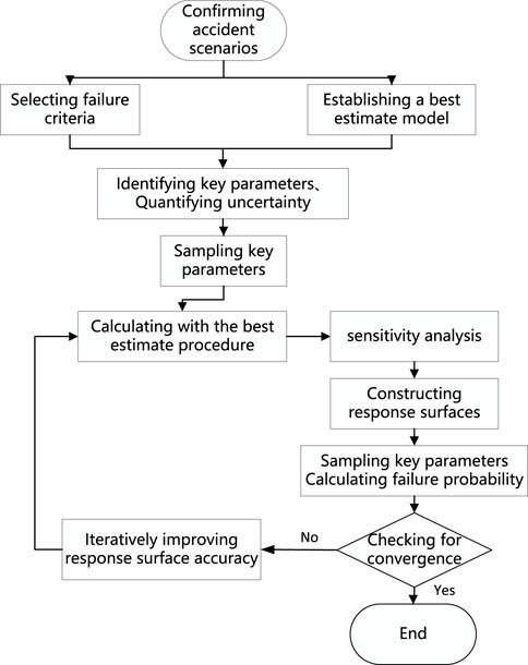
Figure 1. Schematic diagram of the reliability analysis for passive systems.

First, the passive system is identified, and its functions, failure criteria, and performance indicators are clarified, laying the foundation for subsequent simulations. Second, a best-estimate code is developed that complies with internationally recognized guidelines and is consistent with prior information. Third, the relevant parameters affecting system uncertainty are defined, and uncertainty is screened, labeled, and quantified based on the available information. The randomness is described using probability density functions, and the sampling method is determined.

Fourth, parameter sampling is performed, and the sample size is determined based on reliability and confidence requirements. The sampling results are grouped to form an input matrix. Fifth, the input matrix is integrated into the developed model and the best-estimate code is executed. Sixth, the performance indicators of each model are calculated, and an output vector is generated. Seventh, the reliability of the passive safety system is analyzed. Eighth, a new input vector is obtained using the sampling method, and its corresponding performance indicators and output vector are obtained through the response surface (step nine). Subsequent work is to determine whether the calculation converges and to improve the calculation accuracy.

3 System modeling and analysis

3.1 System modeling

This paper uses VITARS as the best-estimate code to model and calculate. Referring to the overall VITARS coolant system model developed by Lu Guoqing (Liu, 2015), the reactor core, pressurizer, steam generator, and secondary-side passive residual heat removal system relevant to this problem are remodeled based on the requirements of this study.

The passive residual heat removal system studied in this paper is an important measure for preventing severe accidents in the advanced pressurized water reactor. In the event of a loss of feedwater to the steam generator or the station black-out accident combined with the failure of auxiliary feedwater steam-driven pumps, the reactor cooling system is no longer capable of continuously removing heat, resulting in a sharp rise in the reactor temperature and pressure to rise continuously, and thus preventing the normal operation of the residual heat removal system (Wang et al., 2012). In this emergency situation, the PRS system is activated. The height difference between the PRS heat exchanger and the steam generator forms a natural circulation, passively removing the core decay heat and the stored heat of various equipment in the reactor coolant system, further reducing the primary circuit temperature and pressure, and thus avoiding a loss-of-coolant accident that may be caused by primary circuit overpressure. In addition, a cooling water tank is set outside the containment to provide sufficient cooling water for the heat exchanger, ensuring that the PRS system can continue to operate self-sustainably for 72 h after an accident, providing valuable buffer time for accident management and emergency response. The secondary-side passive residual heat removal system is installed on the secondary side of the steam generator in all three coolant loops. The VITARS modeling diagram is shown in Figure 2.

Figure 2

Figure 2. Node diagram of passive heat removal system.

3.2 Simulation study on the station black-out accident combined with the failure of auxiliary feedwater steam-driven pumps

Based on the aforementioned characteristic parameters, the formed debris bed in its natural state exhibits a significant extent of spreading. With an increase in the mass of molten material, the proportion of large-sized fragments in the formed debris bed also increases. Under the constant pressure conditions, as the subcooling of water decreases, the proportion of large-sized fragments in the debris bed increases. Since the molten material is sufficiently cooled in water, the high-temperature impact on the bottom plate of the water tank is relatively small.

In this simulation, to better understand the safety performance of nuclear power plants under extreme conditions and to provide a scientific basis for preventing and responding to similar accidents, we assume that both the auxiliary feedwater system and the emergency core cooling system fail after the accident occurs. Therefore, the residual heat of the reactor will be mainly removed by the PRS system.

The accident sequence is shown in Table 1.

Table 1

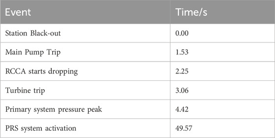
Table 1. Sequence of events for station blackout with auxiliary feedwater steam-driven pump failure.

Figures 3, 4 show the water level of the cooling water tank and the peak temperature of the coolant outlet over the entire 72 h after the accident, respectively. Figure 3 shows that the water in the cooling water tank is nearly depleted at around 70 h, while Figure 4 shows that the coolant outlet temperature has not shown an upward trend, indicating that the water volume setting of the PRS cooling water tank is sufficient. In addition, the reactor outlet temperature reaches its peak within 1 h, which means that the analysis of the results within 1 h has already covered the most dangerous situation of the reactor. In subsequent batch calculations, in order to save time, only the reactor parameter response in the first hour is calculated.

Figure 3

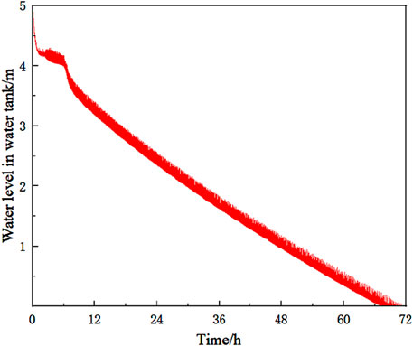
Figure 3. Water level in heat exchanger water tank within 72 h after reactor trip.

Figure 4

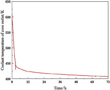
Figure 4. Coolant temperature of core outlet within 72 h after reactor trip.

During this process, the temperature of the outermost layer of the fuel cladding never exceeds 672K, and the coolant in the core region is always in a liquid state, and the core is not exposed, indicating that the core is always in a safe state. Within 72 h after the accident, the outlet temperature of the reactor coolant can be reduced to nearly 400K, and natural circulation can be maintained in both the primary and secondary sides of the fluid, so it is considered that the reactor coolant system has entered a safe state.

4 Reliability analysis of PRS

4.1 Critical parameters and failure criteria

Critical parameters are those that have the greatest impact on system performance. They can generally be divided into operating parameters and structural parameters. For the secondary-side passive residual heat removal system, based on literature research and expert judgment, the input parameters that need to be considered are shown in Table 2.

Table 2

Table 2. Summary of critical parameters and their statistical distributions.

Since the distribution ranges of general system critical parameters (such as heat transfer area) are not completely symmetrical, their actual parameter ranges may deviate from the standard normal distribution. In this case, a truncated normal distribution is more reasonable, and its distribution is shown in Figure 5.

Figure 5

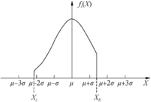
Figure 5. Probability density function of a truncated normal distribution.

Therefore, the normal distributions used in this paper are all truncated normal distributions, and the probability density function can be expressed as ψ(μ,σ,a,b;x), and the specific expression is as shown in the Equation 6:

$\psi \left(\overline{\mu },\overline{\sigma },a,b;x\right)=\left\{\begin{array}{ll}0& x\le a;\\ \frac{\varphi \left(\overline{\mu },{\overline{\sigma }}^{2}x\right)}{\mathrm{\Phi }\left(\overline{\mu },{\overline{\sigma }}^2;b\right)-\mathrm{\Phi }\left(\overline{\mu },{\overline{\sigma }}^2;a\right)}& a<x<b;\\ 0& b\le x.\end{array}\right.(6)$

where $\overline{\mu }$ and $\overline{\sigma }$ are the mean and standard deviation, respectively, of the standard normal distribution; a and b are the lower and upper bounds, respectively, of the truncated normal distribution parameter values.

In the reliability analysis of passive systems, the most important step is to determine the failure criterion of the system. For the PRS system studied in this paper, its key task is to remove the decay heat generated after the reactor shutdown through natural circulation under the accident conditions, and to reduce the coolant temperature and the pressure of the primary cooling system timely and effectively, preventing the occurrence of local boiling in the coolant inside the core, and thus ensuring the integrity of the reactor core cladding (Wang, 2022). Therefore, this study takes the peak temperature of the coolant at the core outlet as the failure criterion of the PRS system. The failure region can be determined as shown in the Equation 7:

$F=\left\{\mathrm{\Omega }:{\mathrm{T}}_{peak}>618\mathrm{K}\right\}(7)$

After determining the uncertainty of the critical parameters, Latin Hypercube Sampling (LHS) is employed to sample the critical parameters listed in Table 2. According to the research object, the key parameters mainly come from PRS heat exchangers (PRHX).

LHS draws samples from the entire distribution of random variables and produces more stable and reliable results. In other words, LHS can obtain good sampling results with fewer samples (Huang and Kuang, 2012).

After sampling, a self-written script is used to batch modify the relevant parts of the key parameters in the input cards, and 100 groups of input cards are obtained. Then, the VITARS program is used to calculate these 100 groups of input cards, and the operating data of the reactor is obtained. The output parameters of interest are extracted, and finally, the input parameters and corresponding output parameters of each calculation are grouped as a set for subsequent analysis.

4.2 Computational analysis of sample data

Preliminary batch calculations were conducted, and the results are shown in Figure 6. It was found that within the range of uncertain parameters, the coolant outlet temperature generally reached its peak at around 500 s, with the peak temperature fluctuating slightly around 592 K, which is far below the failure temperature. Therefore, an attempt was made to find the worst-case condition within the range of uncertain parameters to determine whether the PRS system had a probability of failure within the range of uncertainty. After a series of sampling and calculations, the worst-case condition within the range of uncertainty was found, and the coolant temperature response without the PRS system was calculated. A comparison of the two is shown in Figure 7. The results come from small batches simulations using Thermal-Hydraulic programs.

Figure 6

Figure 6. Curve of coolant temperature of core outlet.

Figure 7

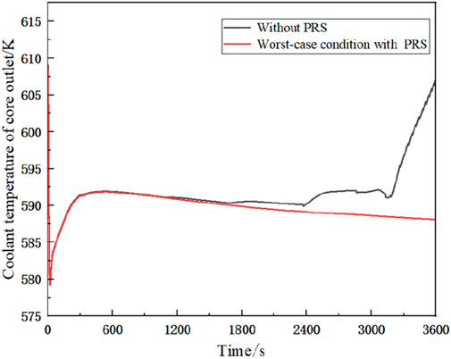
Figure 7. Comparison of coolant outlet temperature with and without PRS.

Without PRS system, the coolant outlet temperature began to rise at around 1800 s. This was due to the loss of all feedwater, causing the water in the steam generator to continuously boil while absorbing the heat generated by the core. Finally, the water evaporated at around 1,800 s, and the coolant lost its ultimate heat sink, leading to a temperature increase. The reactor coolant would then begin to boil. However, under the worst-case condition with the PRS system, where the peak temperature of the coolant outlet is highest within the uncertainty parameter range, the friction factor and inlet/outlet resistance coefficient in the heat exchanger tubes were both at their maximum values within the range of uncertainty. Due to tube blockage, the effective flow area was at its minimum value. Due to scaling, the tube thickness increased, and the initial temperature of the heat exchanger water tank was 40°C. Even under these conditions, the PRS system could still effectively remove the heat generated by the core. According to the calculations, the coolant outlet temperature would not rise again within 72 h, and the water in the tank would not be depleted. Therefore, it can be concluded that the PRS is not prone to failure within the range of uncertain parameters and has superior safety.

Therefore, some extreme conditions are superimposed to further test the reliability of PRS system. The coolant temperature decreases due to the opening of the steam generator safety valve and the pressure drop. Therefore, it is feasible to delay the opening of the steam generator safety valve. Considering the maximum allowable pressure of the steam generator, the delay opening time is limited to within 1 min.

4.3 Sensitivity analysis

Before establishing the response surface, sensitivity analysis is needed to compare the importance of each input parameter to the output parameters. Input parameters with relatively low importance can be directly set to fixed values after sensitivity analysis, thereby reducing the model complexity and minimizing the interference of unnecessary input parameters on the model. In this paper, Spearman’s rank correlation coefficient is selected as the basis for sensitivity analysis.

Spearman’s rank correlation coefficient is used to estimate the strength of the correlation between two random variables and is generally represented by ρ. Its value ranges from [-1, 1]. The stronger the correlation between the two variables, the closer the absolute value of the rank correlation coefficient is to 1. A positive value indicates a positive correlation, a negative value indicates a negative correlation, and a value close to 0 indicates no correlation (Chen et al., 2013).

Sensitivity analysis was performed on the above input parameters and corresponding output parameters, and the results are shown in Figure 8. The output parameter is the failure criterion, which is the peak temperature of the coolant outlet.

Figure 8

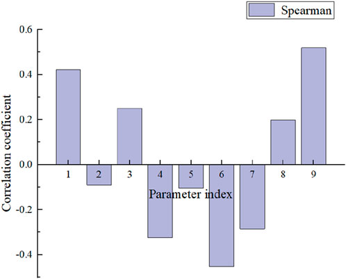
Figure 8. Sensitivity analysis results.

Parameters numbered 1, 4, 6, and 9 are the reactor power, PRHX tube diameter, initial water temperature of the cooling water tank, and safety valve delay opening time, respectively. These four parameters have a strong correlation with the output parameters and are selected as the input parameters for response surface training. Given the significant differences in magnitudes among the various feature variables, normalization is necessary to mitigate their impact when used as training data for a response surface model.

5 Response surface methodology and reliability analysis

Batch calculations are performed to obtain the training data for the response surface. To test the effectiveness of the response surface, 100 groups of data are divided into 90 training sets and 10 test sets.

5.1 Polynomial response surface

The order of the highest-order term of the polynomial response surface can be selected according to the relationship between the response value and the input parameters. In general, the operation of a passive system is more complex, and a first-order model cannot accurately predict its operating results. Therefore, a second-order model is selected to establish the response surface model here (Kirchsteiger and Lavín, 2004).

Using the above 100 groups of data for training and testing, a self-written script is written for regression analysis, and the final result of the quadratic polynomial response surface is obtained as shown in Equation 8:

$\begin{array}{l}Y\left(X\right)=477.74-0.04X_0+2509.91X_1+0.54X_2-0.01X_3\\ -0.83X_0{X}_1-10.61X_1{X}_2-0.72X_1{X}_3+16434.8X_1^2\end{array}(8)$

where $X_0$ is the reactor power; $X_1$ is the PRHX tube diameter; $X_2$ is the initial water temperature of the cooling water tank; $X_3$ is the safety valve delay opening time.

5.2 Neural network response surface

When constructing a multi-layer neural network, a issue that needs attention is the number of hidden layers and the number of nodes in the hidden layer. The hidden layer plays an abstracting role and is responsible for extracting key features from the input parameters, and the number of nodes in the hidden layer directly determines the size and capacity of the network.

To enhance the ability of the neural network to process information, adding hidden layers is an effective way. However, this will also lead to an increase in the complexity of the training process, thus requiring more training data and a longer training period. For the response surface model of this problem, in order to replace the complex thermo-hydraulic program, efforts should be made to reduce the scale of the network structure in order to reduce the length of the training time. Generally, a BP neural network with a three-layer structure is already able to meet the needs of most response surface models. Based on these factors, this study chose to construct a neural network model with only a single hidden layer (Wang et al., 2025).

For the regression problem of this topic, a three-layer BP neural network is selected. The number of neurons in the input layer is 4, the number of neurons in the hidden layer is 9, and the number of neurons in the output layer is 1, which can be expressed as N (4, 9, 1), and the structure is shown in Figure 9. The optimal number of hidden layer neurons is obtained using Bayesian optimization. The principle of Bayesian optimization is based on Bayes’ theorem. First, a probability model of the objective function is constructed, and then this probability model is continuously updated with new sampling points. Based on the model, the next most promising sampling point is calculated, so as to efficiently find the optimal solution of the objective function (Pedroni and Zio, 2017; Lu, 2022).

Figure 9

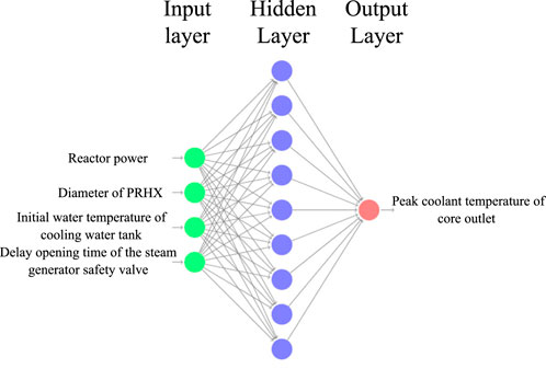
Figure 9. Neural network response surface structure diagram.

After automatic parameter tuning using the Bayesian optimization method, the final configuration determined is that the hidden layer uses PReLU, the output layer uses Linear, and the Adam optimizer is used with an initial learning rate of lr = 0.01. For this neural network response surface, the mean squared error (MSE) is 0.008003.

The Adam optimizer used in this article not only achieves the function of adaptive learning rate, but also has simple implementation, high computational efficiency, and low memory requirements, making it an optimizer with excellent performance (Wang et al., 2018; Helton and Davis, 2003; Ye, 2020; Dong et al., 2024).

PReLU, also known as Parametric Rectified Linear Unit, is an improvement on ReLU. As shown in Figure 10, it introduces a learnable slope parameter on the negative half-axis, where represents the output of the previous layer. This design enables neurons to remain in an activated state even when the input is negative, effectively avoiding the “neuron death” problem that may be caused by excessive gradients during the backpropagation process of ReLU. In addition, PReLU also demonstrates many advantages such as high computational efficiency and stable gradient propagation, making it suitable for most deep learning tasks.

Figure 10

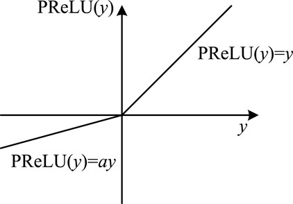
Figure 10. PReLU image.

5.3 Prediction result comparison

After the establishment and training of the response surface model, it is necessary to compare the prediction capabilities of the two response surfaces. By sampling 5,000 times for the input parameters and distributions determined in Section 3.5, new input samples are obtained and substituted into the established quadratic polynomial response surface and neural network response surface for calculation. Using the 100 groups of data generated by VITARS and the 5,000 groups of data output by each response surface, probability distribution diagrams as shown in Figure 11 and cumulative probability distribution diagrams as shown in Figure 12 are plotted.

Figure 11

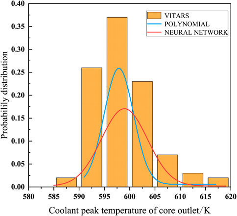
Figure 11. Probability distribution of coolant temperature of core outlet.

Figure 12

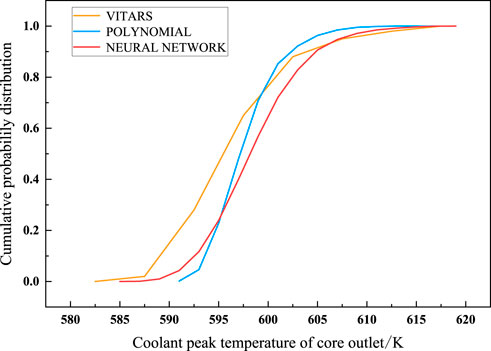
Figure 12. Cumulative probability distribution of coolant temperature of core outlet.

From Figure 11, it can be seen that similar to the VITARS calculation data, the output results of the two response surfaces approximately follow a normal distribution, and the probability peak appears between 595K and 600K. However, compared with the quadratic polynomial response surface, the neural network can better cover the parameter range of the training set, reflecting the true distribution of the data. For the cumulative probability distribution in Figure 12, due to the scarcity of VITARS data samples, the cumulative distribution has abrupt changes and is not smooth, but the output of the neural network response surface is still very close to the VITARS data, and is sufficiently approximate the true distribution curve. In contrast, the cumulative distribution of the quadratic polynomial response surface lacks a temperature range of about 10K, which is significantly different from the actual distribution. Although the limited sample of the VITARS data results in abrupt changes rather than smooth transitions in its cumulative distribution, the output of the neural network response surface is still more similar to the VITARS data.

To further compare the differences in the fitting capabilities of the two response surface models, the input parameters of the original 100 groups of data are used as the input of the response surface, and the predicted values output by the two response surfaces are compared with the real output of VITARS. In Figure 13, a Parity plot is shown, which is a scatter plot that compares the differences between the model results and the baseline data. A baseline is added to the figure to represent the perfect prediction value of the model. When the predicted point of the model falls on the baseline, it means that the prediction error of the model at that point is 0, and the farther away from this line, the greater the error. In addition, an error interval is also drawn. The predicted values of the neural network response surface are all within the 1% error interval, while only 90% of the predicted results of the quadratic polynomial are within the error interval, which indicates that the prediction capability of the neural network response is also better than that of the quadratic polynomial.

Figure 13

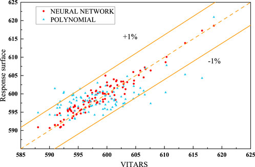
Figure 13. Comparison of prediction accuracy between two response surfaces.

In general, the prediction results of the neural network response surface can well reflect the probability distribution characteristics of the parameters, and compared with the baseline values, the error can be controlled within 1%, which can meet the large-scale and high-precision calculation requirements of the passive system reliability analysis.

5.4 Failure probability calculation

Based on the above comparison, the neural network response surface with better prediction performance is adopted as the surrogate model of VITARS. After extracting 5,000, 10,000, 50,000, 100,000, and 200,000 groups of sampling data using Latin hypercube sampling, the trained neural network response surface is used for prediction. To reduce the impact of different results for each sampling, each group of calculations is performed 5 times, and the average value of the results is taken. The failure probability is summarized in Table 3. It can be seen that the failure probability converges at 100,000 calculations, and the failure probability is 0.035%, which is acceptable. The prediction results of 10,000 and 100,000 times are shown in Figure 14.

Table 3

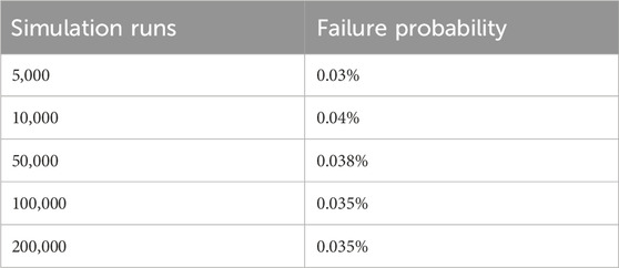
Table 3. Failure probability.

Figure 14

Figure 14. Neural network calculation results. (A) Sample size = 10,000. (B) Sample size = 100,000.

6 Conclusion

This paper conducts a reliability analysis on the passive residual heat removal system of the typical large advanced pressurized water reactor. The main findings and conclusions are summarized as follows:

(1) Two response surface models were established to predict the peak temperature of the reactor coolant outlet, including a quadratic polynomial response surface and a neural network response surface. A comparative study was conducted on the performance of the two response surfaces. The neural network response surface model is more suitable as a surrogate model for the VITARS code, with higher prediction accuracy. The error in the predicted peak coolant outlet temperature can be controlled within 1%.

(2) A reliability analysis was performed on the PRS. The VITARS code was used to model the PRS, and then Latin hypercube sampling was used to obtain samples, which were input into the VITARS code for calculation. Within the range of parameter uncertainty, the PRS can ensure very high reliability under the accident condition of the station black-out accident combined with auxiliary feedwater steam-driven pump failure. Only under extreme conditions, such as the additional delayed opening of the steam generator safety valves, is there a possibility of failure.

(3) After an extra-delayed opening of the steam generator safety valve, the trained neural network response surface was used to calculate the coolant outlet peak temperature for 100,000 samples. Under extreme conditions, the final failure probability is 0.035%, which is acceptable.

Data availability statement

The raw data supporting the conclusions of this article will be made available by the authors, without undue reservation.

Author contributions

TL: Writing–original draft. XK: Writing–review and editing. GL: Writing–review and editing. SC: Writing–review and editing. RC: Writing–review and editing. WT: Writing–review and editing.

Funding

The author(s) declare that no financial support was received for the research, authorship, and/or publication of this article.

Conflict of interest

The authors declare that the research was conducted in the absence of any commercial or financial relationships that could be construed as a potential conflict of interest.

The author(s) declared that they were an editorial board member of Frontiers, at the time of submission. This had no impact on the peer review process and the final decision.

Generative AI statement

The author(s) declare that no Generative AI was used in the creation of this manuscript.

Publisher’s note

All claims expressed in this article are solely those of the authors and do not necessarily represent those of their affiliated organizations, or those of the publisher, the editors and the reviewers. Any product that may be evaluated in this article, or claim that may be made by its manufacturer, is not guaranteed or endorsed by the publisher.

References

Au, S. K., and Beck, J. L. (2003). Subset simulation and its application to seismic risk based on dynamic analysis. J. Eng. Mech. 129 (8), 901–917. doi:10.1061/(asce)0733-9399(2003)129:8(901)

CrossRef Full Text | Google Scholar

Burgazzi, L. (2012). Performance assessment of a passive system as a non-stationary stochastic process. Nucl. Eng. Des. 248, 301–305. doi:10.1016/j.nucengdes.2012.03.022

CrossRef Full Text | Google Scholar

Chen, J., Zhou, T., Liu, L., and Wang, Z. L. (2013). Comparison of reliability analysis methods for passive safety systems. Huadian Technol. 35 (2), 14–17+20+83. doi:10.3969/j.issn.1674-1951.2013.02.007

CrossRef Full Text | Google Scholar

Dong, C., Zhang, C., He, G., Zhang, Z., Cong, J., Meng, Z., et al. (2024). 3D topology optimization design of air natural convection heat transfer fins. Nucl. Eng. Des. 429, 113623. doi:10.1016/j.nucengdes.2024.113623

CrossRef Full Text | Google Scholar

Helton, J. C., and Davis, F. J. (2003). Latin hypercube sampling and the propagation of uncertainty in analyses of complex systems. Reliab. Eng. and Syst. Saf. 81 (1), 23–69. doi:10.1016/s0951-8320(03)00058-9

CrossRef Full Text | Google Scholar

Huang, C. F., and Kuang, B. (2012). Preliminary study on reliability evaluation methods for passive safety systems. Nucl. Saf. 1 (1), 35–41+79. doi:10.3969/j.issn.1672-5360.2012.01.009

CrossRef Full Text | Google Scholar

Jafari, J., D’Auria, F., Kazeminejad, H., and Davilu, H. (2003). Reliability evaluation of a natural circulation system. Nucl. Eng. Des. 224 (1), 79–104. doi:10.1016/s0029-5493(03)00105-5

CrossRef Full Text | Google Scholar

Kirchsteiger, C., and Lavín, R. B. (2004). Best links between PSA and passive safety systems reliability. EUR: European Commission, 1–15.

Google Scholar

Liu, Q. (2015). Reliability analysis of AP1000 passive safety system based on neural network method. Beijing, China: Tsinghua University. Master's thesis.

Google Scholar

Lu, G. Q. (2022). Development and application of a visual interactive nuclear power system analysis program. Xi'an, China: Master's thesis.

Google Scholar

Marquès, M., Pignatel, J., Saignes, P., D’Auria, F., Burgazzi, L., Müller, C., et al. (2005). Methodology for the reliability evaluation of a passive system and its integration into a Probabilistic Safety Assessment. Nucl. Eng. Des. 235 (24), 2612–2631. doi:10.1016/j.nucengdes.2005.06.008

CrossRef Full Text | Google Scholar

Mezio, F. (2010). Assessment of the thermo-hydraulic phenomenology of an isolation condenser and its impact on the nuclear safety. Master Thesis Instituto Balseiro. S. C. de Bariloche,Argentina. doi:10.13182/t130-43351

CrossRef Full Text | Google Scholar

Nayak, A. K., Gartia, M. R., Antony, A., Vinod, G., and Sinha, R. K. (2008). Passive system reliability analysis using the APSRA methodology. Nucl. Eng. Des. 238 (6), 1430–1440. doi:10.1016/j.nucengdes.2007.11.005

CrossRef Full Text | Google Scholar

Pedroni, N., and Zio, E. (2017). An Adaptive Metamodel-Based Subset Importance Sampling approach for the assessment of the functional failure probability of a thermal-hydraulic passive system. Appl. Math. Model. 48, 269–288. doi:10.1016/j.apm.2017.04.003

CrossRef Full Text | Google Scholar

Wang, B. S., Wang, D. Q., Jiang, J., and Zhang, J. M. (2012). Evaluation of functional failure probability of passive safety systems based on adaptive importance sampling method. Nucl. Power Eng. 33 (2), 30–36. doi:10.3969/j.issn.0258-0926.2012.02.007

CrossRef Full Text | Google Scholar

Wang, C. Y. (2022). Research on reliability analysis methods for marine passive residual heat removal systems. Harbin, China: Harbin Engineering University.

Google Scholar

Wang, C. Y., Peng, M. J., Xia, G. L., and Cong, T. L. (2018). Reliability analysis of integrated passive residual heat removal system for pressurized water reactor. J. Harbin Eng. Univ. 39 (12), 1910–1917. doi:10.11990/jheu.201708056

CrossRef Full Text | Google Scholar

Wang, J., Du, C., Yan, F., Hua, M., Gongye, X., Yuan, Q., et al. (2025). Bayesian optimization for hyper-parameter tuning of an improved twin delayed deep deterministic policy gradients based energy management strategy for plug-in hybrid electric vehicles. Appl. Energy 381, 125171. doi:10.1016/j.apenergy.2024.125171

CrossRef Full Text | Google Scholar

Xie, G. F., He, X. H., Tong, J. J., and Zheng, Y. H. (2007). Calculation of failure probability of residual heat removal system physical process of HTR-10 by response surface method. Acta Phys. Sin. 6 (6), 3192–3197. doi:10.7498/aps.56.3192

CrossRef Full Text | Google Scholar

Ye, Q. (2020). Optimal estimation and uncertainty analysis of small break loss of coolant accident in small reactors. Wuhan, China: Master's thesis, Huazhong Univ. of Sci. and Tech.

Google Scholar