A new theoretical performance analysis method considering longitudinal and transverse end effects for flat linear induction magnetohydrodynamic pumps

The flat linear induction pumps (FLIPs) are a class of driving devices that converts electromagnetic energy into mechanical energy of pumped liquid metal, which are widely used in the field of energy power and chemical industries. The end effects and wall eddy current effect of FLIPs can significantly reduce the pump head and energy conversion efficiency. In this paper, the longitudinal and transverse end effects of FLIPs caused by the finite length of the core were analyzed, and the analytical expressions of the electromagnetic field in the electromagnetic air gap were given. Based on the mathematical analysis of the end effects and the T-shaped equivalent circuit of the rotary induction motor, an equivalent circuit model was established, considering two kinds of end effects and wall eddy current effects. The calculation methods of main characteristic parameters, such as head and energy conversion efficiency, were given. The accuracy of the analytical model was validated by comparing the calculation results with the open experimental data. The work can provide a rapid analysis method for improving the energy conversion efficiency and working performance of FLIPs.

1 Introduction

Liquid metal is widely used as coolant in advanced energy systems such as solar concentrator systems, fast breeder reactors, fusion reactors, and accelerator-driven systems because of its great thermal physical and flow properties (Gnanasekaran, 2022). Due to corrosive of liquid metals, these energy systems have a high requirement for the tightness and corrosion resistance of the power pumps. Therefore, it is possible to consider the use of induction magnetohydrodynamic (MHD) pumps which do not contain mechanical moving parts to pump the fluid (Zhao et al., 2022). According to the structure of the pump ditch, the induction MHD pumps can be divided into Flat linear induction pumps (FLIPs), Annular linear induction pumps (ALIPs), and Helical induction pumps (HIPs) (Baker and Tessier, 1987). However, despite the advantages of such induction pumps, such as simple structure and reliable operation, the energy conversion efficiency of most induction MHD pumps designed so far is much lower than that of conventional mechanical pumps. Therefore, it is very important to study the working performance of induction MHD pumps, such as output head and energy conversion efficiency.

The induction pumps can be seen as a special linear induction motor, which converts electrical energy into mechanical energy of the fluid through the magnetic field. Numerical simulations are often used to solve such complex flow and heat transfer problems (Dong et al., 2024; Hou et al., 2024; Hou et al., 2025; Zhang et al., 2024). Some of them take into account the effect of the end effect (Smolyanov and Karban, 2018; Uskov et al., 2016). The former proposed a numerical optimization algorithm for the double-sided linear induction pump, considering the saturation effect and transverse end effect of the core. The latter established a two-dimensional numerical model of FLIP considering transverse and longitudinal end effects, and studied the influence of different winding structures on pump head. In addition to the end effect, the operating temperature (Sharma et al., 2019) and geometric structure (Dong et al., 2013) also significantly affects the performance of MHD pumps. The research results show that the head and efficiency of ALIPs decrease obviously with the increase of temperature and magnetic gap thickness.

However, the complex magnetic field in the pump ditch makes the numerical model unable to realize the rapid calculation of the induction pump performance. Compared with numerical simulation, analytical models are more suitable for quickly understanding and optimizing the energy conversion mechanism under complex magnetic fields (Hasani and Irani Rahaghi, 2022; Kortas et al., 2015; Wang et al., 2024; Zhang et al., 2020). The Chinese Institute of Mechanics (Qiu, 1964) has conducted a comprehensive theoretical study on various types of electromagnetic pumps. Based on the method of magnetohydrodynamics, three independent models have been established to analyze the longitudinal end effect, transverse end effect and wall eddy current effect of FLIPs, respectively. However, the accuracy of these electromagnetic pump models is low. Subsequently, studies have proposed a method that can simultaneously consider the longitudinal and transverse end effects of FLIPs (Dronnik et al., 1979). However, this model does not consider the effect of wall eddy current and short circuit strip, and only applies to the current source power supply. Liu et al. (2023) built a one-dimensional analytical model, considering only the longitudinal end effect and the wall eddy current effect.

The liquid metal pumped by the induction pumps can be regarded as the secondary of the induction motors, so the equivalent circuit models established for the linear induction motors (Amiri and Mendrela, 2014; Duncan, 1983; Kahourzade et al., 2021; Lu et al., 2008; Naderi et al., 2020) are often used in the analytical calculation of the induction pumps. The equivalent circuit model can be applied to both voltage source and current source. By establishing an ALIP equivalent circuit model considering dynamic end effect, it is found that the correction of longitudinal end effect can significantly reduce the relative error in the range of high flow rate (Lo Pinto et al., 2023). Wang et al. (2019) also makes a theoretical analysis of the characteristics of ALIP based on the equivalent circuit method, and considers the gravity effect. Zhang et al. (2022) used the improved equivalent circuit model to establish the one-dimension field analytical model of ALIP, considering the longitudinal end effect and the wall eddy current effect, and gave the analytical expressions of each end effect component of the main physical parameters.

From the literature review, it can be found that compared with ALIPs, FLIPs lack a relatively complete theoretical model that can comprehensively consider the longitudinal end effect, the transverse end effect, and the wall eddy current effect. In addition, most of the literatures focus on the effective output power of FLIPs, and the relationship between the energy conversion efficiency and the electromagnetic characteristics of the pumps has not been fully studied. In this work, the transverse and longitudinal end effects of FLIPs are analyzed, and the specific expressions of the main electromagnetic field parameters are derived. The influences of longitudinal and transverse end effects on electromagnetic field distribution, head and energy conversion efficiency of FLIPs are discussed respectively. Then, based on the mathematical analysis of the end effects, several correction factors that consider the longitudinal alone and the transverse end effects alone are derived. The impedance of each part of FLIPs is modified by correction factors of the end effects, and an equivalent circuit model is established, considering the two kinds of end effects, the wall eddy current effect, and the effect of short circuit strips. Finally, the calculated results of the equivalent circuit model under different voltages and operating temperatures are compared with the experimental data, the accuracy and universality of the established equivalent circuit model are validated.

2 Characteristics and basic principle of FLIPs

Figure 1 shows the main structure and basic principled diagram of FLIPs. The FLIPs are mainly composed of two parts, one part is mainly composed of iron core and coil, also known as primary. The iron core is usually stacked with silicon steel sheets to reduce eddy current losses. The other part is secondary composed of the pump trench wall, liquid metal, and short circuit strips. The short circuit strip is generally made of copper sheet with excellent conductive performance, which mainly increases the induced current in the liquid metal and thus increases the electromagnetic driving force and weakens the influence of the transverse end effect to a certain extent.

Figure 1

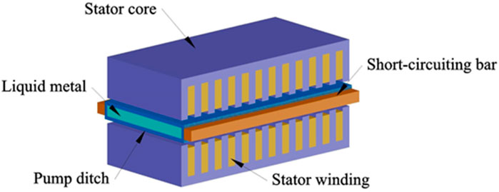
Figure 1. Schematic diagram of the FLIP.

When the three-phase AC current is connected to the winders on both sides, the magnetic field moving along the axis of the pump groove will be generated in the air gap of FLIP, which also known as the traveling wave magnetic field. Under the action of the traveling wave magnetic field, the current will be induced in the liquid metal according to the law of electromagnetic induction. The interaction of the induced current with the traveling wave magnetic field creates a Lorentz force that pushes the liquid metal forward.

Because the length and width of the core are finite, the breakage of the core at both sides has an effect on the distribution of magnetic field in the air gap, which is often referred to as the end effects. The end effects of FLIP can be divided into longitudinal and transverse end effects. On the one hand, the iron core is limited in the length direction, so there are inflow and outflow end for the fluid, which will change the amplitude of the magnetic field along the flow direction, a phenomenon known as the dynamic longitudinal end effect. In addition, the asymmetry of the three-phase impedance will be introduced, which in turn leads to the static longitudinal end effect. On the other hand, the length of the core in the width direction is also limited, which will cause leakage flux in the lateral side end, which is known as the first type of transverse end effect. In addition, the longitudinal component of the current in the liquid metal can also lead to a saddle-shaped distribution of the air-gap magnetic field in the width direction, which is known as the second type of transverse end effect.

3 Mathematical analysis of end effects of FLIP

3.1 Longitudinal end effect

In the specific case of FLIP, the conveying medium is incompressible fluid with constant conductivity, the fluid velocity is much less than the speed of light, and the electromagnetic frequency is below 1000 Hz (the displacement current can be completely ignored). Therefore, Maxwell’s equations and its constitutive equations can be modified into the following form:

$\left.\begin{array}{l}\nabla \times \mathit{H}=\mathit{J}\\ \nabla \times \mathit{E}=-\frac{\mathrm{\partial }\mathit{B}}{\mathrm{\partial }t}\\ \nabla \cdot \mathit{B}=0\\ \mathit{B}=\mu \mathit{H}\\ \mathit{J}=\sigma \left(\mathit{E}+\mathit{V}\times \mathit{B}\right)\end{array}\right\}(1)$

Where H is the magnetic field intensity (A/m), J is the electric current density (A/m²), E is the electric field intensity (V/m), B is the magnetic induction intensity (T), u is the permeability of the medium, σ is the conductivity of the medium (S/m), V is the fluid velocity (m/s).

Based on Equation 1, the magnetic vector potential A is introduced. And add the following two equations:

$\left.\begin{array}{l}\mathit{B}=\nabla \times \mathit{A}\\ \mathit{E}=-\frac{\partial \mathit{A}}{\partial t}\end{array}\right\}(2)$

The longitudinal end effect is directly related to the performance and characteristics of FLIP, and theoretical analysis is carried out below. In order to simplify the mode, some basic assumptions are introduced as follows.

1) The permeability of stator core is infinite, and the conductivity is zero.

2) The eddy current effect and the saturation effect of stator core are ignored. In addition, the skin effect in liquid metal is also not considered.

3) The cogging effect is represented by the jammed coefficient, ignoring the saturation effect and hysteresis loss of the core.

4) The power input frequency and current are three-phase symmetric, and all physical quantities are considered as sinusoidal functions of time t and position x.

5) Since the air gap is very thin, the variation of the air gap magnetic field along the y direction is ignored.

6) The liquid metal flow is incompressible, and its velocity has only a longitudinal component v_x.

The FLIP can be regarded as the unfolded ALIP, so the one-dimensional field model of FLIP considering longitudinal end effect is similar to ALIP (Zhang et al., 2022). Figure 2 shows a bilateral FLIP model considering longitudinal end effects alone. The whole model is divided into three calculation regions which includes entrance region I, coupling region (effective region) II, and exit region III. Based on the principle of equality of magnetomotive force (Ku et al., 1985), the primary magnetic potential is replaced by a surface current layer j_s (x, t). The upstream region of the inlet and the downstream region of the outlet are also represented by the virtual current layers j_k1 and j_k3 in the plural form. When the surface current layer j_s (x, t), j_k1 and j_k3 on one side are considered as zero, all the formulas are applicable to FLIPs in the form of single-sided winding arrangement.

Figure 2

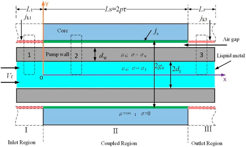
Figure 2. Longitudinal end-effect model.

The traveling-wave current layer of the three regions is defined as

$\left.\begin{array}{l}{j}_{\mathrm{k}1}=j{\sigma }_{13}{E}_{\mathrm{z}1}x<0\\ j_{\mathrm{s}}=J_{\text{smax}}{\mathrm{e}}^{\mathrm{j}\left(\omega t-kx\right)}0<x<L_{\mathrm{s}}\\ j_{\mathrm{k}3}=j{\sigma }_{13}{E}_{\mathrm{z}3}x>L_{\mathrm{s}}\end{array}\right\}(3)$

Where j is the imaginary symbol. k = π/τ is the wave number, τ is the pole pitch (m). J_smax is the amplitude of the traveling wave current layer (A/m). J_smax = $\sqrt{2m_1{N}_1{k}_{\mathrm{w}1}{I}_1}$, m₁ is the number of phases, N₁ is the winding per pole per phase series parameter, k_w1 is the fundamental winding factor, I₁ is the phase current of each branch of the winding (A), p is the logarithm of the poles. ω is the angular velocity (rad/s), L_s is the effective region length (m), E_z1 and E_z3 represent the electric field intensities in the corresponding regions. σ₁₃ is the virtual conductivity in regions I and III.

${\sigma }_{13}={0.73}^2/\left(g_{\mathrm{e}}\omega {\mu }_0\right)=k_{\mathrm{f}}^2{g}_{\mathrm{e}}/\left(\omega {\mu }_0\right)$

Where, g_e is the half-thickness of the electromagnetic air gap (m), u₀ is the vacuum permeability,k_f = 0.73/g_e.

As shown in Figure 2, the reference coordinates are fixed at the primary. According to assumptions (1) and (5), along rectangular loop paths 1, 2, and 3 in regions I, II, and III, it is obtained by applying Abe’s loop theorem:

$\frac{g_{\mathrm{e}}}{u_0}\frac{\partial }{\partial x}\left(B_{\mathrm{y}1}\right)=j_{\mathrm{f}1\mathrm{z}}+j_{\mathrm{k}1}+j_{\mathrm{w}1z}x<0(4)$

$\frac{g_{\mathrm{e}}}{u_0}\frac{\partial }{\partial x}\left(B_{\mathrm{y}2}\right)=j_{\mathrm{f}2\mathrm{z}}+j_s+j_{\mathrm{w}2\mathrm{z}}0<x<L_{\mathrm{s}}(5)$

$\frac{g_{\mathrm{e}}}{u_0}\frac{\partial }{\partial x}\left(B_{\mathrm{y}3}\right)=j_{\mathrm{f}3\mathrm{z}}+j_{\mathrm{k}3}+j_{\mathrm{w}3\mathrm{z}}x>L_{\mathrm{s}}(6)$

Where B_y1, B_y2, and B_y3 are the magnetic field intensities in regions I, II, III, j_f1z, j_f2z, j_f3z are the z components of the line induction current density of liquid metal in the corresponding regions, respectively. j_w1z, j_w2z, j_w3z are the z components of the line induction current density of the wall in the corresponding regions, respectively.

The magnetic vector potential A of each region can be defined as

$\left.\begin{array}{l}{A}_{\mathrm{z}1}=A_{11}\left(x\right)e^{\mathrm{j}wt}x<0\\ A_{\mathrm{z}2}=A_{22}\left(x\right)e^{\mathrm{j}wt}0<x<L_s\\ A_{\mathrm{z}3}=A_{33}\left(x\right)e^{\mathrm{j}wt}x>L_s\end{array}\right\}(7)$

From Equations 1, 2 and 7, Formulas 4–6 can be written separately as

$\frac{g_{\mathrm{e}}}{{\mu }_0}\frac{d^2{A}_{11}}{d{x}^2}-{\sigma }_{\mathrm{f}}{d}_{\mathrm{f}}{\nu }_{\mathrm{f}}\frac{d{A}_{11}}{dx}-\left(\mathrm{j}\omega {\sigma }_{\mathrm{f}}{d}_{\mathrm{f}}\left(1+k_{\mathrm{w}}\right)-\omega {\sigma }_{13}\right)A_{11}=0(8)$

$\frac{g_{\mathrm{e}}}{{\mu }_0}\frac{d^2{A}_{33}}{d{x}^2}-{\sigma }_{\mathrm{f}}{d}_{\mathrm{f}}{\nu }_{\mathrm{f}}\frac{d{A}_{33}}{dx}-\left(\mathrm{j}\omega {\sigma }_{\mathrm{f}}{d}_{\mathrm{f}}\left(1+k_{\mathrm{w}}\right)-\omega {\sigma }_{13}\right)A_{33}=0(9)$

$\frac{g_{\mathrm{e}}}{{\mu }_0}\frac{d^2{A}_{22}}{d{x}^2}-{\sigma }_{\mathrm{f}}{d}_{\mathrm{f}}{\nu }_{\mathrm{f}}\frac{d{A}_{22}}{dx}-\mathrm{j}\omega {\sigma }_{\mathrm{f}}{d}_{\mathrm{f}}\left(1+k_{\mathrm{w}}\right)A_{22}=-J_{s\max }{e}^{\mathrm{j}kx}(10)$

Where, k_w = σ_fd_f/σ_wd_w is the wall eddy current coefficient, which represents the eddy current effect of the conductive pump ditch wall. d_w is the pump channel wall thickness (m). σ_f is the fluid conductivity (S/m), 2d_f is the pump channel thickness (m), ν_f is the fluid velocity (m/s).

The solutions of Equations 8–10 can be written as

$\left.\begin{array}{l}{A}_{11}\left(x\right)=c_{11}{e}^{r_{\mathrm{k}1}x}x<0\\ A_{22}\left(x\right)=c_{\mathrm{t}}{e}^{-\mathrm{j}kx}+c_{21}{e}^{r_{\mathrm{c}21}x}+c_{22}{e}^{r_{\mathrm{c}22}x}0<x<L_{\mathrm{s}}\\ A_{33}\left(x\right)=c_{33}{e}^{r_{\mathrm{k}3}x}x>L_{\mathrm{s}}\end{array}\right\}(11)$

Where c₁₁, c₂₁, c₂₂, c₃₃ are the integration constants depending on the boundary conditions. G is the quality factor of the pump, which reflects the ability of pump to convert one type of energy into another. R_m is the magnetic Reynolds number, which characterizes the dynamics of the MHD. s is the slip, s = (v_s-v_f)/v_s. v is the traveling wave velocity, v_s = 2pτ.

From Equations 1, 7 and 11 the distribution of magnetic field B_y1, B_y2, B_y3 and electric field E_z1, E_z2, E_z3 in the three regions can be written as

$\left.\begin{array}{l}{B}_{\mathrm{y}1}=-r_{\mathrm{k}1}{c}_{11}{e}^{r_{\mathrm{k}1}}x<0\\ B_{\mathrm{y}2}=B_{\mathrm{y}2\mathrm{c}t}+B_{\mathrm{y}2\mathrm{c}1}+B_{\mathrm{y}2\mathrm{c}2}0<x<L_{\mathrm{s}}\\ B_{\mathrm{y}3}=-r_{\mathrm{k}1}{c}_{11}{e}^{r_{\mathrm{k}1}}x>L_{\mathrm{s}}\end{array}\right\}(12)$

Where, B_y2ct = jkc_te^j(ωt-kx), B_y2c1 = -c₂₁e^rc21x+jωt, B_y2c2 = -c₂₂e^rc22x+jωt represent the no-end effect component, the inlet end effect component and the outlet end effect component, respectively.

$\left.\begin{array}{l}{E}_{\mathrm{z}1}=-\mathrm{j}\omega c_{11}{e}^{r_{\mathrm{k}1}x+\mathrm{j}\omega t}x<0\\ E_{\mathrm{z}2}=-\mathrm{j}\omega c_{\mathrm{t}}{e}^{\mathrm{j}\left(\omega t-kx\right)}-\mathrm{j}\omega c_{21}{e}^{r_{\mathrm{c}21}x+\mathrm{j}\omega t}-\mathrm{j}\omega c_{22}{e}^{r_{\mathrm{c}22}x+\mathrm{j}\omega t}0<x<L_{\mathrm{s}}\\ E_{\mathrm{z}3}=-\mathrm{j}\omega c_{12}{e}^{r_{\mathrm{k}3}x+\mathrm{j}\omega t}x>L_{\mathrm{s}}\end{array}\right\}(13)$

On the boundary line between regions I, II, and III (x = 0, x = L_s), tangential magnetic field continuity and tangential electric field continuity should be satisfied.

$\begin{array}{l}{B}_{\mathrm{y}1}{|}_{x=0}=B_{\mathrm{y}2}{|}_{x=0}{B}_{\mathrm{y}2}{|}_{x=L_{\mathrm{s}}}=B_{\mathrm{y}3}{|}_{x=L_{\mathrm{s}}}\\ E_{\mathrm{z}1}{|}_{x=0}=E_{\mathrm{z}2}{|}_{x=0}{E}_{\mathrm{z}2}{|}_{x=L_{\mathrm{s}}}=E_{\mathrm{z}3}{|}_{x=L_{\mathrm{s}}}\end{array}(14)$

From Equations 12–14, the specific expressions for c₁₁, c₂₁, c₂₂, c₃₃ can be solved. The detailed expressions are listed in the Supplementary Appendix section.

3.2 Transverse end effect

The inner core of ALIP is a cylinder, and the outer core is a ring, so the iron core of ALIP is broken only in the length direction. However, the core of FLIP is limited in the length direction and width direction, so there are both longitudinal end effect and transverse end effect, and the theoretical analysis and characteristic calculation of FLIP are more complex. Figure 3 shows the analytical model of FLIP considering only the transverse end effect.

Figure 3

Figure 3. Transverse end effect model.

The whole model is divided into liquid metal region I, pump trench wall region II and short circuit strip region III. The definition of the equivalent current layer js is consistent with the longitudinal end-effect coupling region. Ignoring the influence of the longitudinal end effect, the basic assumption of the model that considers the transverse end effect is basically consistent with the longitudinal end effect.

According to Assumption (4) and (5), the form of the magnetic field B in coupling region is defined as

$B_{\mathrm{y}1}=B_1\left(z\right)e^{\mathrm{j}\left(\omega t-kx\right)}(15)$

Where B_y1 is the y components of air gap flux density in the region I.

Along rectangular loop paths 1 in regions I, it is obtained by applying Abe’s loop theorem

$\frac{g_{\mathrm{e}}}{{\mu }_0}\frac{\partial }{\partial z}\left(B_{\mathrm{y}1}\right)=-j_{\mathrm{f}x}-j_{\mathrm{w}1\mathrm{x}}(16)$

Similarly, it can be obtained in the longitudinal section:

$\frac{g_{\mathrm{e}}}{{\mu }_0}\frac{\partial }{\partial z}\left(B_{\mathrm{y}1}\right)=j_{\text{fz}}+j_{\mathrm{w}1\mathrm{z}}-j_{\mathrm{s}}(17)$

Where j_fx, j_fz are distributed to represent the x-direction and z-direction components of the current density of the liquid metal wire in the upper half of region I, j_w1x and j_w1z are distributed to represent the x-direction and z-direction components of the half-line current density of the pump trench pipeline in region I.

Simultaneous Equations 1, 16, 17, which are obtained after collation:

$\frac{{\partial }^2}{\partial x^2}\left(B_{\mathrm{y}1}\right)+\frac{{\partial }^2}{\partial z^2}\left(B_{\mathrm{y}1}\right)-\frac{{\mu }_0{\sigma }_{\text{fs}}{V}_{\mathrm{x}}}{\delta }\frac{\partial }{\partial x}\left(B_{\mathrm{y}1}\right)-\frac{{\mu }_0{\sigma }_{\text{fs}}}{\delta }\frac{\partial }{\partial t}\left(B_{\mathrm{y}1}\right)-\frac{{\mu }_0{\sigma }_{\text{ws}}}{\delta }\frac{\partial }{\partial t}\left(B_{\mathrm{y}1}\right)=-\frac{{\mu }_0}{g_{\mathrm{e}}}\frac{\partial }{\partial x}\left(j_{\mathrm{s}}\right)(18)$

Where, σ_fs = σ_f d_f is Surface conductivity.

From Equations 3, 15, Formula 18 can be written as

$\frac{{\partial }^2}{\partial z^2}\left[B_1\left(z\right)\right]-\left[k^2+\mathrm{j}\frac{\omega {\mu }_0{\sigma }_{\text{fs}}}{\delta }\left(s+k_{\mathrm{w}І}\right)\right]B_1\left(z\right)=\mathrm{j}\frac{k{\mu }_0}{g_{\mathrm{e}}}{J}_{\text{smax}}(19)$

Where k_wⅠ = σ_w d_w/σ_f d_f is the eddy current effect coefficient in region I. Similarly, in regions II and III can be obtained as

$k_{\mathrm{w}\pi }={\sigma }_{\mathrm{w}}\left(d_{\mathrm{w}}+d_{\mathrm{f}}\right)/{\sigma }_{\mathrm{f}}{d}_{\mathrm{f}},k_{\mathrm{w}ш}={\sigma }_{\mathrm{s}}{d}_{\mathrm{s}}/{\sigma }_{\mathrm{f}}{d}_{\mathrm{f}}$

In the fluid region, B₁(z) is an even function with respect to z. Thus, the full solution form of Equation 19 is given as Equation 20:

$B_{\mathrm{y}1}\left(x,z,t\right)=\left[B_1\cosh \left({\alpha }_{1}z\right)+c{t}_1\right]e^{\mathrm{j}\left(\omega \mathrm{t}-\text{kx}\right)}(20)$

Where B₁ is the integration constant to be determined.

${\alpha }_1^2=k^2+\mathrm{j}\frac{\omega {\mu }_0{\sigma }_{\text{fs}}}{g_{\mathrm{e}}}\left(s+k_{\mathrm{w}І}\right)$

$c{t}_1=\frac{-\mathrm{j}{\mu }_0{J}_{\text{smax}}}{k{g}_{\mathrm{e}}\left[1+\mathrm{j}G\left(s+k_{\mathrm{w}І}\right)\right]}$

From Equations 17, 18, 20, the z and x components of the line current density of liquid metal (j_fz, j_fx) and wall (j_w1z, j_w1x) in region I can be written as, respectively

$\left.\begin{array}{l}{j}_{\text{fz}}=\frac{1}{1+k_{\mathrm{w}\mathrm{{\rm I}}}}\left[{\epsilon }_1{B}_1\cosh \left({\alpha }_{1}z\right)+c_{\mathrm{j}1}\right]e^{\mathrm{j}\left(\omega t-kx\right)}\\ j_{\text{fx}}=\frac{-g_{\mathrm{e}}{\alpha }_1}{{\mu }_0\left(1+k_{\mathrm{w}\mathrm{{\rm I}}}\right)}{B}_1\sinh \left({\alpha }_{1}z\right)e^{\mathrm{j}\left(\omega t-kx\right)}\\ j_{\mathrm{w}1z}=\frac{1}{1+k_{\mathrm{w}\mathrm{{\rm I}}}}\left[{\epsilon }_{\mathrm{w}1}{B}_1\cosh \left({\alpha }_{1}z\right)+c_{\mathrm{w}1}\right]e^{\mathrm{j}\left(\omega t-kx\right)}\\ j_{\mathrm{w}1x}=\frac{-k_{\mathrm{w}1}{g}_{\mathrm{e}}{\alpha }_1}{{\mu }_0\left(1+k_{w\mathrm{{\rm I}}}\right)}{B}_1\sinh \left({\alpha }_{1}z\right)e^{\mathrm{j}\left(\omega t-kx\right)}\end{array}\right\}$

Combining Equation 20 and the fifth equation in maxwell’s Equation 1, the z components and x components of the electric field intensity in region I are obtained in the following forms:

$E_{z1}=\frac{1}{{\sigma }_{\text{fs}}{k}_{\mathrm{w}\mathrm{{\rm I}}}\left(1+k_{\mathrm{w}\mathrm{{\rm I}}}\right)}\left[{\epsilon }_{\mathrm{w}1}{B}_1\cosh \left({\alpha }_{1}z\right)+c_{\mathrm{w}1}\right]e^{\mathrm{j}\left(\omega t-kx\right)}$

$E_{\mathrm{x}1}=\frac{-g_{\mathrm{e}}{\alpha }_1}{{\mu }_0{\sigma }_{\text{fs}}\left(1+k_{\mathrm{w}\mathrm{{\rm I}}}\right)}{B}_1\sinh \left({\alpha }_{1}z\right)e^{\mathrm{j}\left(\omega t-kx\right)}$

Since the walls of the two sides of the pump communication channel and short circuit strip are located outside the core, the induced magnetic field generated by the current can be ignored. The magnetic field in region II is considered to be zero, then:

$\nabla \times \mathit{E}=0(21)$

Curl the fifth equation in maxwell’s Equation 1 and then combine it with Equation 21:

$\frac{\mathit{\partial }}{\mathit{\partial }x}\left(j_{\mathrm{w}2\mathrm{z}}\right)-\frac{\mathrm{\partial }}{\mathrm{\partial }z}\left(j_{\mathrm{w}2\mathrm{x}}\right)=0(22)$

Where, j_w2z, j_w2x are the z components and x components of the current density in the pipe line of the pump trench wall in the upper half of region II, respectively.

According to the current continuity theorem:

$\frac{\partial }{\partial x}\left(j_{\mathrm{w}2\mathrm{x}}\right)+\frac{\partial }{\partial z}\left(j_{\mathrm{w}2\mathrm{z}}\right)=0(23)$

Take the derivative of Equations 22, 23 with respect to x and y, respectively, and add them together:

$\frac{{\partial }^2}{\partial x^2}\left(j_{\mathrm{w}2\mathrm{z}}\right)+\frac{{\partial }^2}{\partial z^2}\left(j_{\mathrm{w}2\mathrm{z}}\right)=0(24)$

The general solution of Equation 24 is given as Equation 25:

$j_{\mathrm{w}2\mathrm{z}}=\left[A_1{e}^{kz}+A_2{e}^{-kz}\right]e^{\mathrm{j}\left(\omega t-kx\right)}(25)$

Where A₁ and A₂ are the integration constants to be determined.

From Equations 23, 25, j_w2x can be written as

$j_{\mathrm{w}2\mathrm{x}}=\mathrm{j}\left[A_2{e}^{-kz}-A_1{e}^{kz}\right]e^{\mathrm{j}\left(\omega t-kx\right)}(26)$

Combining Equations 25, 26, and the fifth equation in maxwell’s Equation 1, the z components and x components of the electric field intensity in region II are obtained in the following forms:

$E_{\mathrm{z}2}=\frac{1}{{\sigma }_{\text{fs}}{k}_{\mathrm{w}\pi }}\left[A_1{e}^{kz}+A_2{e}^{-kz}\right]e^{\mathrm{j}\left(\omega t-kx\right)}$

$E_{x2}=\frac{\mathrm{j}}{{\sigma }_{\text{fs}}{k}_{\mathrm{w}\pi }}\left[A_2{e}^{-kz}-A_1{e}^{kz}\right]e^{\mathrm{j}\left(\omega t-kx\right)}$

There is also no magnetic field in region III, so the resolution process is similar to that in region II. Thus, the expressions for each component of the induced eddy current and electric field in region III can be written as

$j_{\mathrm{s}3\mathrm{z}}=\left[A_3{e}^{kz}+A_4{e}^{-kz}\right]e^{\mathrm{j}\left(\omega t-kx\right)}$

$j_{\mathrm{s}3\mathrm{x}}=\mathrm{j}\left[A_4{e}^{-kz}-A_3{e}^{kz}\right]e^{\mathrm{j}\left(\omega t-kx\right)}$

$E_{\mathrm{z}3}=\frac{1}{{\sigma }_{\text{fs}}{k}_{\mathrm{w}ш}}\left[A_3{e}^{kz}+A_4{e}^{-kz}\right]e^{\mathrm{j}\left(\omega t-kx\right)}$

$E_{\mathrm{x}3}=\frac{\mathrm{j}}{{\sigma }_{\text{fs}}{k}_{\mathrm{w}ш}}\left[A_4{e}^{-kz}-A_3{e}^{kz}\right]e^{\mathrm{j}\left(\omega t-kx\right)}$

Where j_s3z, j_s3x are the z components and x components of the current density of the short-circuiting bar in the upper half of region III, respectively. E_3z, E_3x are the z components and x components of the electric field in region III, respectively.

The complex integration constants B₁, A₁, A₂, A₃, and A₄ in the solution process need to be determined through boundary conditions. Tangential electric field continuity and normal current continuity should be satisfied on the boundary lines of the pump groove wall in contact with liquid metal and short circuit strip (z = c and z = c + t_w), respectively. In addition, it should be satisfied that the normal current at the outer boundary of the short circuit strip (z = c + t_w + t_s) is zero. The form of the boundary conditions can be written as

$\begin{array}{l}{E}_{\mathrm{x}1}{|}_{\mathrm{z}=\mathrm{c}}=E_{\mathrm{x}2}{|}_{\mathrm{z}=\mathrm{c}}{j}_{\text{fz}}+j_{\mathrm{w}1\mathrm{z}}{|}_{\mathrm{z}=\mathrm{c}}=j_{\mathrm{w}2\mathrm{z}}{|}_{\mathrm{z}=\mathrm{c}}\\ E_{\mathrm{x}2}{|}_{\mathrm{z}=\mathrm{c}+{\mathrm{t}}_{\mathrm{w}}}=E_{\mathrm{x}3}{|}_{\mathrm{z}=\mathrm{c}+{\mathrm{t}}_{\mathrm{w}}}{j}_{\mathrm{w}2\mathrm{z}}{|}_{z=\mathrm{c}+{\mathrm{t}}_{\mathrm{w}}}=j_{\mathrm{s}3\mathrm{z}}{|}_{\mathrm{z}=\mathrm{c}+{\mathrm{t}}_{\mathrm{w}}}\\ j_{s3z}{|}_{z=c+t_w+t_s}=0\end{array}$

The detailed expressions for B₁, A₁, A₂, A₃, and A₄ are listed in the Supplementary Appendix section.

3.3 Results and discussion

The mathematical analysis of longitudinal dynamic end effect and second transverse end effect of FLIP are carried out in Section 3.1, 3.2, respectively. In this section, the influence of longitudinal and transverse end effect on the air gap magnetic field, head and energy conversion efficiency will be further analyzed based on a practical FLIP (Bluhm et al., 1964).

In the literature, the FLIP adopts the arrangement of double-sided core and single-sided winding. This arrangement of pumps is often used in some high temperature application environments because of the low requirement for heat insulation. The operating temperature is 673.15 K and the voltage source is used for power supply. The specific parameters of the FLIP are shown in Table 1.

Table 1

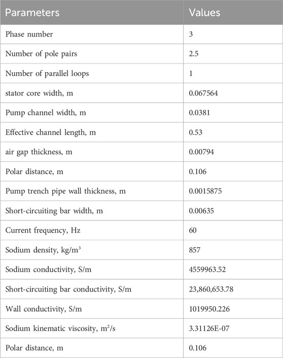
Table 1. The main parameters of the FLIP.

3.3.1 Electromagnetic field distribution

It can be seen from Equation 12 that the magnetic field B_y is divided into three components, B_y1ct, B_y1c1, and B_y1c2, when considering the longitudinal end effect alone. Since the value of B_y1ct is only related to the structure and operation condition of the induction pump and independent of the axial position, it is considered to be a component independent of longitudinal end effect. Similarly, it is possible to separate the magnetic field in Equation 20 into one component without transverse end effects (B_y2ct) and two components with end effects (B_y2c1, B_y2c2).

Figures 4, 5 show the distributions of the magnetic field B_y without and with the longitudinal and transverse end effects, respectively. For different slip conditions, Figure 6A shows the axial distribution (x direction) of the magnetic field amplitude when only the longitudinal end effect is considered, and Figure 6B shows the transverse distribution (z direction) of the magnetic field amplitude when only the transverse end effect is considered. The operating condition of the pump are I = 7.8 A, f = 60 Hz, Q = 1.417,254 m³/h.

Figure 4

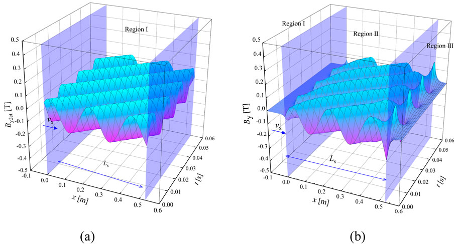
Figure 4. The spatio-temporal distributions of magnetic field. (A) Without considering longitudinal end effect. (B) Considering longitudinal end effect.

Figure 5

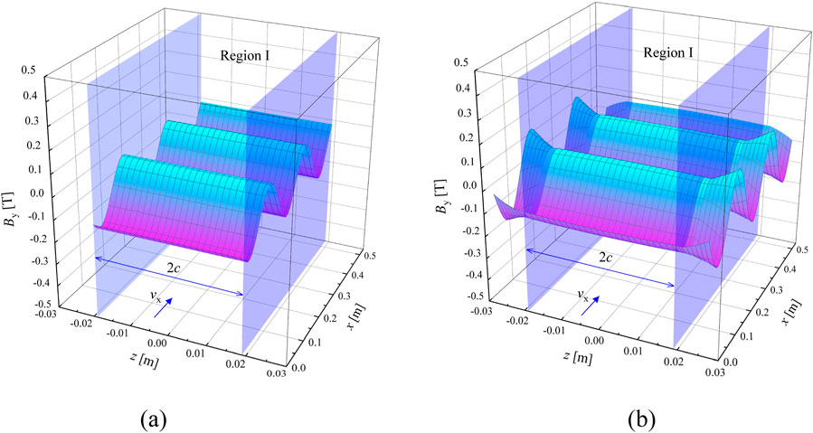
Figure 5. The spatial distribution of the magnetic field B_y. (A) Without considering transverse end effect. (B) Considering transverse end effect.

Figure 6

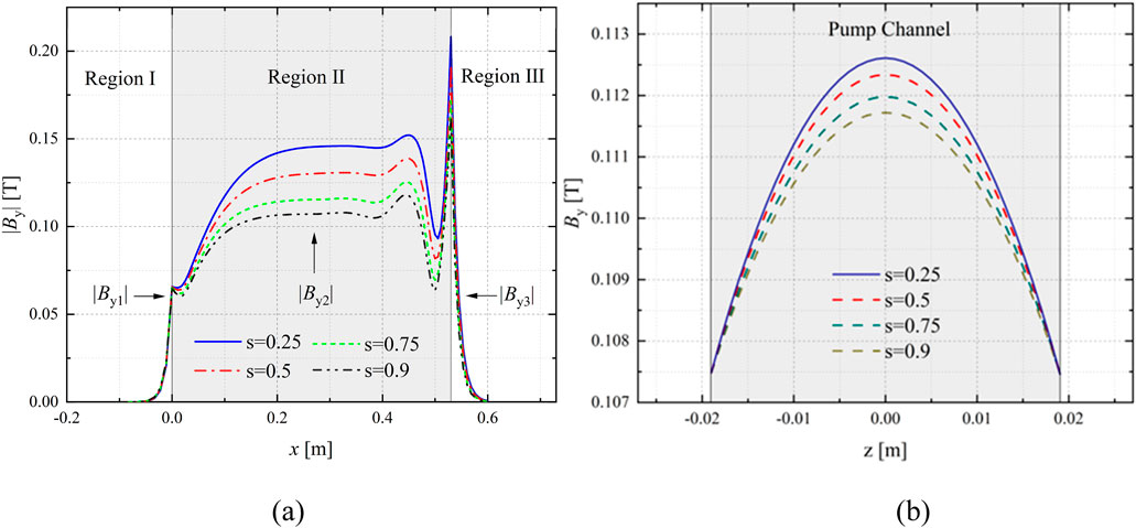
Figure 6. The distribution of the magnetic field amplitude |B_y| considering the end effect for different slip differences. (A) Longitudinal end effect. (B) Transverse end effect.

When the end effects are not considered, as shown in Figure 4A, the magnetic field is a sine wave that propagates along the flow direction x, whose speed is 2fτ. In addition, it can be seen from Figure 5A and Equation 20 that B_y at this time is only related to the structural parameters and operating conditions of the pump, but not to the position in the lateral direction z.

After considering the influence of the inlet and outlet longitudinal end effect components B_y1 and B_y3, the distribution of the air gap magnetic field is shown in Figures 4B, 6A. In the figure, |B_y1| and |B_y3| are the amplitude of the attenuation magnetic field of the inlet and outlet end effect, respectively, and |B_y2| is the amplitude of the synthetic magnetic field in the coupling region II. It is obvious that the air gap magnetic field in the coupling region II is distorted after considering the longitudinal end effect. The magnetic field is weakened on the whole near the entrance region I, while the magnetic field shows a trend of first decreasing and then increasing near the exit region III, and the peak appears at the interface of region I and II. Moreover, in region II and III, the amplitude of the magnetic field increases obviously with the decrease of the slip, while this change is not obvious in region I.

When only transverse end effect is considered, the distribution of the magnetic field in the coupling region of FLIP is shown in Figure 6B for different slip differences. Similar to the slip characteristics of the pump when only the longitudinal end effect is considered, the amplitude of the air gap magnetic field increases with the decrease of the slip, but the change is not large. This is because the lateral end effect is caused by the lateral breaking of the stator core, so its influence on the air gap magnetic field generation is mainly related to the pump geometry and operating conditions. The longitudinal end effect is not only related to the breakage of the core in the longitudinal direction, but also to the inflow and outflow of the liquid metal. Therefore, the amplitude of the air gap magnetic field considering the longitudinal end effect is much more sensitive to the change of the flow rate.

3.3.2 Pressure and energy conversion efficiency

In Sections 3.1, 3.2, the expressions of the magnetic field, electric field and the line current density in each direction of the FLIP have been given when the two end effects are considered respectively. Therefore, it is easy to further calculate the head and efficiency of the FLIP at different currents. When the access phase voltages are 200 V, 150 V, and 100 V, the corresponding phase currents measured are 10.5 A, 7.8 A, and 5.6A, respectively.

Figures 7A, B show the flow-head characteristic curve and flow-efficiency characteristic curve of the FLIP when the longitudinal end effect is considered alone. Figures 8A, B show the flow-head characteristic curve and flow-efficiency characteristic curve, respectively, when the transverse end effect is considered alone.

Figure 7

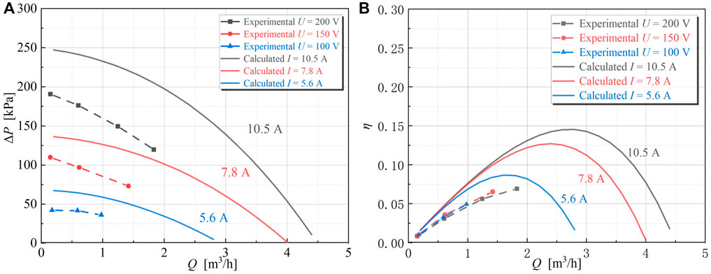
Figure 7. Comparison between calculated and experimental values of longitudinal end effect model. (A) ΔP-Q (B) η-Q.

Figure 8

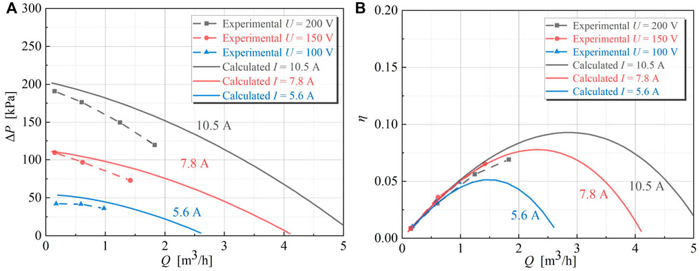
Figure 8. Comparison between calculated and experimental values of transverse end effect model. (A) ΔP-Q (B) η-Q.

As can be seen in Figure 7, considering longitudinal alone, the calculated results of the head and efficiency are significantly higher than the experimental values. The average error of head is 40.91% and the average error of efficiency is 55.01%. From Figure 8, considering transverse end effect alone, the average error is 13% for head and 14% for efficiency. Comparing Figures 7, 8, it can be found that the accuracy of the transverse end effect model is significantly higher than the longitudinal end effect model. This indicates that the transverse end effect has a greater impact on the performance of FLIPs than the longitudinal end effect. In addition, the error levels of both models increase with the flow velocity. This is partly because at high Reynolds numbers the magnetic field exerts extra drag on the flowing liquid metal, thereby suppressing turbulence, which is partly attributed to MHD effect (Rao and Sankar, 2011). Therefore, when the flow rate is high, the actual resistance is greater than the theoretical calculation value, and the experimental value of the head is also lower than the theoretical calculation value.

4 Equivalent circuit model considering end effects

It can be seen from Section 3.3 that the head and energy conversion efficiency of the FLIP cannot be accurately calculated when considering the longitudinal end effect alone and the transverse end effect alone. In order to comprehensively consider the two end effects, in this section, an equivalent circuit model of the FLIP is developed based on the mathematical analysis of the end effects in Section 3.1, 3.2. In the equivalent circuit model, the longitudinal end effect correction factor K and the transverse end effect correction factor C are used to represent the influence of the two end effects on each impedance. The equivalent circuit model can be used for both current and voltage source supply. The specific structure of the model is shown in Figure 9.

Figure 9

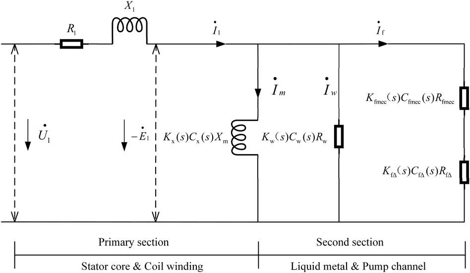
Figure 9. Schematic diagram of equivalent circuit model of FLIP.

From Figure 9, on the primary section, R₁ is the ideal equivalent resistance of the primary winding (Ω), X₁ is the ideal leakage reactance of the primary winding (Ω), U₁ is the winding phase voltage (V), I₁ is the winding phase current (A). On the second section, R_w is the ideal equivalent resistance of wall and short circuit strips (Ω), R_f is the ideal equivalent resistance of liquid metal (Ω), X_m is the ideal magnetizing reactance (Ω), I_m is the magnetizing current (A), I_w is the total induced current in the wall and short-circuit strips (A), I_f is the induced current in the liquid metal (A). K, C are the longitudinal and transverse end-effect correction factors corresponding to each resistance, respectively. The ideal Impedance parameters can be written as

$R_1=\frac{2L_{\text{cp}}{N}_1}{{\sigma }_{\mathrm{c}}{S}_{\mathrm{c}}}$

$X_1=1.58\frac{f}{100}{\left(\frac{N_1}{100}\right)}^2\frac{2a}{pq}\left({\lambda }_{\mathrm{s}}+{\lambda }_{\mathrm{t}}+{\lambda }_{\mathrm{e}}+{\lambda }_{\mathrm{d}}\right)$

$X_{\mathrm{m}}=\frac{4m_1{\mu }_{0}a{V}_{\mathrm{s}}{\left(k_{\mathrm{w}1}{N}_1\right)}^2}{\pi p{g}_{\mathrm{e}}}(27)$

$R_{\mathrm{w}}=\frac{4m_{1}c{\left(k_{\mathrm{w}1}{N}_1\right)}^2}{{\sigma }_{\text{sf}}{k}_{\mathrm{w}}p\tau }$

$R_{\text{fmec}}=\frac{4m_{1}c{\left(k_{\mathrm{w}1}{N}_1\right)}^2}{{\sigma }_{\text{fs}}{k}_{\mathrm{w}}p\tau }$

$R_{\mathrm{f}\Delta }=\frac{4m_{1}c{\left(k_{\mathrm{w}1}{N}_1\right)}^2}{p\tau }$

Where, L_cp is the stator winding average half-turn length (m), σ_c is the conductivity of the wire (S/m), S_c is the cross-sectional area of the wire (m²), λ_s is the slot leakage resistance factor, λ_t is the tooth end leakage resistance coefficient, λ_e is the leakage reactance coefficient at the end of the primary winding, λ_d is the harmonic leakage reactance coefficient.

4.1 Derivation of the longitudinal end effect coefficient

Based on the analytical model in Section 3.1, the total complex power S_i1 transferred from the primary to the secondary and the air gap can be divided into three parts. The complex power S_i2 generated by the equivalent current layer j_s in the coupling area II, the complex power S_ik1 and S_ik3 generated by the equivalent virtual current layer in the upstream area I of the inlet and the downstream area III of the outlet. The three-part complex power can be written as

$S_{\mathrm{i}2}=2c{\int }_0^{L_{\mathrm{s}}}-j_{\mathrm{s}}^{*}{E}_{\mathrm{z}2}dx=P_{\mathrm{i}2}+\mathrm{j}{Q}_{\mathrm{i}2}$

$S_{\text{ik}1}=2c{\int }_{-L_1}^0-j_{\mathrm{k}1}^{*}{E}_{\mathrm{z}1}dx=P_{\text{ik}1}+j{Q}_{\text{ik}1}$

$S_{\text{ik}3}=2c{\int }_{L_{\mathrm{s}}}^{L_{\mathrm{s}}+L_3}-j_{\mathrm{k}3}^{*}{E}_{\mathrm{z}3}dx$

Therefore, the total complex power S_i1 can be written as

$S_{\mathrm{i}1}=S_{\mathrm{i}2}+S_{\text{ik}1}+S_{\text{ik}3}=P_{\mathrm{i}1}+\mathrm{j}{Q}_{\mathrm{i}1}(28)$

The secondary induced electromotive force (EMF) E₁ can be calculated using Equation 28.

$\stackrel{·}{E_1}=-S_{\mathrm{i}1}/\left(m_1\stackrel{·}{I_1}\right)$

Therefore, the excitation reactance X́_m considering the longitudinal end effect can be calculated using the total reactive power of the primary input secondary:

$X_{\mathrm{m}}^{\prime }=m_1{\left|{\dot{E}}_1\right|}^2{Q}_{\mathrm{i}1}(29)$

From X_m in Equation 27 and X^́_m in Equation 29, the correction factor K_x for the excitation reactance considering the longitudinal end effect can be written as

$K_{\mathrm{x}}=X_{\mathrm{m}}^{\prime }/X_{\mathrm{m}}$

The Joule heat P_w of the upper half of the pump ditch pipe can be calculated using the wall eddy current j_w:

$P_{\mathrm{w}}=\frac{c}{{\sigma }_{\mathrm{s}}{k}_{\mathrm{w}\mathrm{{\rm I}}}}\left({\int }_{-L_1}^0{j}_{\mathrm{w}1}^{*}\times j_{\mathrm{w}1}dx+{\int }_0^{L_{\mathrm{s}}}{j}_{\mathrm{w}2}^{*}\times j_{\mathrm{w}2}dx+{\int }_{L_{\mathrm{s}}}^{L_{\mathrm{s}}+L_3}{j}_{\mathrm{w}3}^{*}\times j_{\mathrm{w}3}dx\right)(30)$

The wall resistance $R_{\mathrm{w}}^{\prime }$ and correction factor K_w(s) considering the longitudinal end effect can be written as

$R_{\mathrm{w}}^{\prime }=m_1\left|E_1^2\right|/P_{\mathrm{w}},K_{\mathrm{w}}=R_{\mathrm{w}}^{\prime }/R_{\mathrm{w}}$

The power of liquid metal is mainly divided into mechanical power P_mec and thermal power P_rf. The calculation of P_rf is similar to the Joule heat of the wall in Equation 30.

$P_{\text{rf}}=\frac{c}{{\sigma }_{\mathrm{s}}{k}_{\mathrm{w}\mathrm{{\rm I}}}}\left({\int }_{-L_1}^0{j}_{\mathrm{f}1}^{*}\times j_{\mathrm{f}1}dx+{\int }_0^{L_{\mathrm{s}}}{j}_{\mathrm{f}2}^{*}\times j_{\mathrm{f}2}dx+{\int }_{L_{\mathrm{s}}}^{L_{\mathrm{s}}+L_3}{j}_{\mathrm{f}3}^{*}\times j_{\mathrm{f}3}dx\right)(31)$

In the pump communication channel, the Lorentz force generated by the interaction of the magnetic field and the induced eddy current is the only driving force for the liquid metal. The time-averaged electromagnetic force density f_em(x) can be written as

$f_{\text{em}}\left(x\right)=-\frac{\text{Re}\left[j^{*}\times B\right]}{2d_{\mathrm{f}}}=f_{\text{em}1}\left(x\right)+f_{\text{em}2}\left(x\right)+f_{\text{em}3}\left(x\right)$

Where, f_em1(x), f_em2(x), f_em3(x) are the time-averaged electromagnetic force densities in regions I, II, III, respectively.

$\left.\begin{array}{l}{f}_{\text{em}1}\left(x\right)=\frac{-R_{\mathrm{e}}\left[j_{\mathrm{f}1}^{\ast }\times B_{\mathrm{y}1}\right]}{2d_{\mathrm{f}}}x<0\\ f_{\text{em}2}\left(x\right)=\frac{-R_{\mathrm{e}}\left[j_{\mathrm{f}2}^{\ast }\times B_{\mathrm{y}1}\right]}{2d_{\mathrm{f}}}0<x<L_{\mathrm{s}}\\ f_{\text{em}3}\left(x\right)=\frac{-R_{\mathrm{e}}\left[j_{\mathrm{f}3}^{\ast }\times B_{\mathrm{y}3}\right]}{2d_{\mathrm{f}}}x>L_{\mathrm{s}}\end{array}\right\}(32)$

The electromagnetic pressure difference between the inlet and outlet ΔP_em can be obtained by integrating the electromagnetic force along the flow direction x:

$\Delta P_{\text{em}}={\int }_l{f}_{\text{em}}\left(x\right)dx(33)$

The mechanical power P_mec of the planar electromagnetic pump considering the longitudinal end effect can be written as

$P_{\text{mec}}=\Delta P_{\text{em}}·Q(34)$

The total impedance of the liquid metal series branch can be written as

${\left(R_{\mathrm{f}}/s\right)}^{\prime }=\frac{m_1{\left|E_1\right|}^2}{P_{\text{mec}}/2+P_{\text{rf}}}(35)$

The current I_f of the liquid metal branch can be obtained according to Ohm’s law:

$\left|I_{\mathrm{f}}\right|=\left|\stackrel{·}{E_1}\right|/{\left(R_{\mathrm{f}}/s\right)}^{\prime }(36)$

From Equations 31, 34–36, the equivalent resistance Ŕ_fmec, Ŕ_fΔ and correction factors K_fmec(s), K_fΔ(s) for the thermal and mechanical power of the liquid metal considering the longitudinal end effect can be written as, respectively

$R_{\text{fmec}}^{\prime }=\frac{P_{\text{mec}}/2}{m_1{I}_{\mathrm{f}}^2},R_{\mathrm{f}\Delta }^{\prime }=\frac{P_{\text{rf}}}{m_1{I}_{\mathrm{f}}^2}$

$K_{\text{fmec}}\left(s\right)=R_{\text{fmec}}^{\prime }/R_{\text{fmec}},K_{\mathrm{f}\Delta }\left(s\right)=R_{\mathrm{f}\Delta }^{\prime }/R_{\mathrm{f}\Delta }$

4.2 Derivation of transverse end effect coefficients

Let the magnetic flux at each pole be ϕ(t), which can be written in the following form:

$\varphi \left(t\right)={\int }_{-c}^c{\int }_0^{\tau }{B}_{\mathrm{y}1}\left(x,z,t\right)dxdz$

The instantaneous value $e_1\left(t\right)$ of the single-side primary per-phase potential can be written as

$e_1\left(t\right)=-W_1{k}_{\mathrm{w}1}\frac{d}{dt}\left[\varphi \left(t\right)\right]=-\sqrt{2}{E}_1{e}^{\mathrm{j}\omega t}(37)$

The total induced EMF E₁ in the non-magnetically conductive air gap in Equation 37 can be written as

$E_1=\frac{\sqrt{2}}{2}\mathrm{j}\omega W_1{k}_{\mathrm{w}1}\varphi \left(t\right)$

Therefore, the complex power S_i1 of the secondary considering the transverse end effect can be obtained as

$S_{\mathrm{i}1}=\frac{m{I}_1\left(-E_1\right)}{2\sqrt{3}}=P_{\mathrm{i}2}+\mathrm{j}{Q}_{\mathrm{i}2}$

Similarly, the excitation reactance X˝_m and its correction factor C_x considering the transverse end effect can be written as

$X_{\mathrm{m}}^{″}=m_1{\left|E_1\right|}^2/Q_{\mathrm{i}2},C_{\mathrm{x}}=X_{\mathrm{m}}^{″}/X_{\mathrm{m}}$

The Joule heat generated by the eddy current effect of the short circuit strip is included in the wall Joule heat, and the total Joule heat P_w of the upper half of the pipe can be written as

$P_{\mathrm{w}}=P_{\mathrm{w}1}+P_{\mathrm{w}2}+P_{s3}$

Where,

$P_{\mathrm{w}1}=\frac{1}{2{\sigma }_{\text{fs}}{k}_{\mathrm{w}1}}{\int }_0^{L_{\mathrm{s}}}{\int }_{-c}^c{j}_{\mathrm{w}1\mathrm{z}}^{*}\times j_{\mathrm{w}1\mathrm{z}}+j_{\mathrm{w}1\mathrm{x}}^{*}\times j_{\mathrm{w}1\mathrm{x}}dzdx$

$P_{\mathrm{w}2}=\frac{1}{{\sigma }_{\text{fs}}{k}_{\mathrm{w}2}}{\int }_0^{L_{\mathrm{s}}}{\int }_c^{c+t_{\mathrm{w}}}{j}_{\mathrm{w}2\mathrm{z}}^{*}\times j_{\mathrm{w}2\mathrm{z}}+j_{\mathrm{w}2\mathrm{x}}^{*}\times j_{\mathrm{w}2\mathrm{x}}dzdx$

$P_{\mathrm{s}3}=\frac{1}{{\sigma }_{\text{fs}}{k}_{\mathrm{w}3}}{\int }_0^{L_{\mathrm{s}}}{\int }_{c+t_{\mathrm{w}}}^{c+t_{\mathrm{w}}+t_{\mathrm{s}}}{j}_{\mathrm{s}3\mathrm{z}}^{*}\times j_{\mathrm{s}3\mathrm{z}}+j_{\mathrm{s}3\mathrm{x}}^{*}\times j_{\mathrm{s}3\mathrm{x}}dzdx$

The wall resistance R˝_w considering transverse end effects and the corresponding correction factor C_w(s) can be written as

$R_{\mathrm{w}}^{″}=m_1{\left|E_1\right|}^2/P_{\mathrm{w}},C_{\mathrm{w}}\left(s\right)=R_{\mathrm{w}}^{″}/R_{\mathrm{w}}$

The liquid metal induced eddy Joule heating P_rf in the upper half of the inner region I can be expressed as

$P_{\text{rf}}=\frac{1}{2{\sigma }_{\text{fs}}}{\int }_0^{L_s}{\int }_{-c}^c{j}_{\text{fx}}^{*}\times j_{\text{fx}}+j_{\text{fz}}^{*}\times j_{\text{fz}})dzdx$

The electromagnetic differential pressure ΔP_em and mechanical power P_mec of the planar electromagnetic pump can be calculated as

$\Delta P_{\text{em}}=\frac{-L_{\mathrm{s}}}{2A_{\mathrm{s}}}{\int }_{-c}^c{j}_{\text{fz}}\times B_{\mathrm{y}1}^{*}dz$

$P_{\text{mec}}=\Delta P_{\text{em}}·Q$

The liquid metal branch resistance (R_f/s)˝ and branch current RMS |I_f| considering the lateral end effect can be expressed as

${\left(R_{\mathrm{f}}/s\right)}^{″}=\frac{m_1{\left|E_1\right|}^2}{P_{\text{mec}}+P_{\text{rf}}}$

$\left|I_{\mathrm{f}}\right|=\left|E_1\right|/{\left(R_{\mathrm{f}}/s\right)}^{″}$

Similar to the longitudinal end effect, the resistance R˝_fmec, R˝_fΔ corresponding to the mechanical and thermal power of the liquid metal considering the transverse end effect, and its corresponding correction factor C_fmec(s), C_fΔ(s) can be expressed as

$R_{\text{fmec}}^{″}=\frac{P_{\text{fmec}}/2}{m_1{I}_{\mathrm{f}}^2},R_{\mathrm{f}\Delta }^{″}=\frac{P_{\text{rf}}}{m_1{I}_{\mathrm{f}}^2}$

$C_{\text{fmec}}\left(s\right)=R_{\text{fmec}}^{″}/R_{\text{fmec}},C_{\mathrm{f}\Delta }\left(s\right)=R_{\mathrm{f}\Delta }^{″}/R_{\mathrm{f}\Delta }$

4.3 Calculation of the main characteristic parameters

Based on the longitudinal end effect correction factor K(s) and transverse end effect correction factor C(s) for each impedance obtained in Sections 4.1, 4.2, each impedance value considering the two end effects can be expressed as

$r_{\mathrm{w}}=K_{\mathrm{w}}\left(s\right)C_{\mathrm{w}}\left(s\right)R_{\mathrm{w}}$

$x_{\mathrm{m}}=K_{\mathrm{x}}\left(s\right)C_{\mathrm{x}}\left(s\right)R_{\mathrm{w}}$

$r_{\text{fmec}}=K_{\text{fmec}}\left(s\right)C_{\text{fmec}}\left(s\right)R_{\text{fmec}}$

$r_{\mathrm{f}\Delta }=K_{\mathrm{f}\Delta }\left(s\right)C_{\mathrm{f}\Delta }\left(s\right)R_{\mathrm{f}\Delta }$

The excitation branch and the secondary total impedance can be expressed as

$Z_2=\frac{1}{\frac{1}{\mathrm{j}{x}_{\mathrm{m}}}+\frac{1}{r_{\mathrm{w}}}+\frac{1}{r_{\text{mec}}+r_{\mathrm{f}\Delta }}}$

The total voltage segment input impedance Z_i can be written as

$Z_{\mathrm{i}}=R_1+{\text{jX}}_1+Z_2$

If the voltage is known, the stator phase current ${\dot{I}}_1$ and the secondary induced electromotive force ${\dot{E}}_1$ can be obtained as

$\left.\begin{array}{l}\stackrel{·}{I_1}=\stackrel{·}{U_1}/Z_{\mathrm{i}}\\ -\stackrel{·}{E_1}=\stackrel{·}{I_1}{Z}_2\end{array}\right\}(38)$

The branch currents ${\dot{I}}_{\mathrm{m}}$, ${\dot{I}}_{\mathrm{w}}$, ${\dot{I}}_{\mathrm{f}}$ can be written as, respectively

$\left.\begin{array}{l}\stackrel{·}{I_{\mathrm{m}}}=-\stackrel{·}{E_1}/\mathrm{j}{x}_{\mathrm{m}}\\ \stackrel{·}{I_{\mathrm{w}}}=-\stackrel{·}{E_1}/r_{\mathrm{w}}\\ \stackrel{·}{I_{\mathrm{f}}}=-\stackrel{·}{E_1}/\left(r_{\text{fmec}}+r_{\mathrm{f}\Delta }\right)\end{array}\right\}(39)$

The total complex power S_i of the single-side winding input can be written as

$S_{\mathrm{i}}=m_1{\left|\stackrel{·}{I_1}\right|}^2{Z}_{\mathrm{i}}=P_{\mathrm{i}}+{\text{jQ}}_{\mathrm{i}}$

Where, P_i and Q_i are the total active and reactive power, respectively.

$P_{\mathrm{i}}=m_1{\left|\stackrel{·}{I_1}\right|}^2·\text{Re}\left[Z_{\mathrm{i}}\right]=P_{\mathrm{r}1}+P_{\text{rw}}+P_{\text{rf}}+P_{\text{mec}}(40)$

$Q_{\mathrm{i}}=m_1{\left|\stackrel{·}{I_1}\right|}^2·\text{Im}\left[Z_{\mathrm{i}}\right]$

Where, P_r1 is the Joule heating of the one-sided winding, P_rw is the Joule heat of the upper half of the wall and the short-circuit strip, P_rf is the liquid metal Joule heat of the upper half, P_mec is half of the total mechanical power of the liquid metal.

The current of each branch has been derived in Equations 38, 39, so the specific expression of the power of each part can be easily derived according to the equivalent circuit model.

$\begin{array}{l}{P}_{\mathrm{r}1}=m_1{\left|{\stackrel{·}{I}}_1\right|}^2{r}_1,P_{\text{rw}}=m_1{\left|{\stackrel{·}{I}}_{\mathrm{w}}\right|}^2{r}_{\mathrm{w}}\\ P_{\text{rf}}=m_1{\left|{\stackrel{·}{I}}_{\mathrm{f}}\right|}^2{r}_{\mathrm{f}\Delta },P_{\text{mec}}=m_1{\left|{\stackrel{·}{I}}_{\mathrm{f}}\right|}^2{r}_{\text{fmec}}\end{array}(41)$

From the mechanical power P_mec in Equation 41, the electromagnetic pressure difference ΔP_em of the electromagnetic pump can be obtained as

$\Delta P_{\text{em}}=2P_{\text{mec}}/Q(42)$

The Darcy-Weisbach formula is adopted for calculating the frictional loss ΔP_m of liquid metal in rectangular pump groove. When the flow regime of the liquid metal is turbulent (Re > 2,320), the explicit form of the Colebrook-White equation (Fang et al., 2011; Hafsi, 2021) is used to solve the resistance coefficient λ.

$\Delta P_{\mathrm{m}}=\lambda \frac{l}{d}\frac{{\rho }_{\mathrm{f}}{v}_{\mathrm{f}}^2}{2}(43)$

$\left.\begin{array}{l}\lambda =64/\text{Re}\text{\hspace{1em}Re}\le 2320\\ \lambda =1.613{\left[\ln \left(0.234{\left(\frac{\Delta }{D_{\mathrm{h}}}\right)}^{1.1007}-\frac{60.525}{R_{\mathrm{e}}^{1.1105}}+\frac{56.291}{R_{\mathrm{e}}^{1.0712}}\right)\right]}^{-2}3000<\text{Re}<{10}^8\end{array}\right\}$

Where, l is the length of the pipe (m), d is the feature size (m), ρ_f is the fluid density (kg/m³), v_f is the average velocity in the fluid tube (m/s), Re = ν_f D_h/ν is the Reynolds number of the liquid metal, D_h is the equivalent diameter of the rectangular flow channel (m), ν is the kinematic viscosity (m²/s), Δ is the absolute roughness (m).

From Equations 42, 43, the head of the planar electromagnetic pump ΔP_d can be obtained as

$\Delta P_{\mathrm{d}}=\Delta P_{\text{em}}-\Delta P_{\mathrm{m}}(44)$

The power factor cosφ can be written as

$\cos \phi =\text{Re}\left[Z_{\mathrm{i}}\right]/Z_{\mathrm{i}}$

From Equations 40, 44, the energy conversion efficiency η of the FLIP can be calculated as

$\eta =\frac{\Delta P_{\mathrm{d}}·Q}{2P_{\mathrm{i}}}$

4.4 Results and discussion

In this section, the accuracy and applicability of all equations of the established equivalent circuit model is checked by means of two sets of experimental data: a) Variable voltage condition and b) Variable temperature condition.

4.4.1 Variable voltage condition

Figure 10 shows the comparison of the calculated and experimental values of head and hydraulic efficiency of the equivalent circuit model under the condition of voltage source supply, which corresponds to Section 4.3.

Figure 10

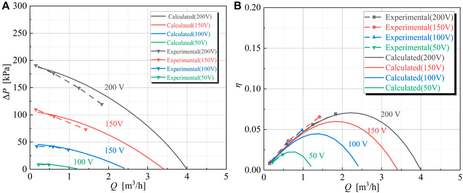
Figure 10. Comparison of the calculated and experimental values of the equivalent circuit model under the voltage power supply condition. (A) ΔP-Q (B) η-Q.

From Equations 32, 33, the calculation of the electromagnetic pressure difference is related to the magnitude of magnetic field amplitude. From the analysis in Section 3.3.1, it can be known that the longitudinal and transverse end effects will inhibit the magnetic field and reduce the magnetic field amplitude. Therefore, Comparing Figures 7, 8, 10, the error level and magnitude of the head and energy conversion efficiency calculation results of the equivalent circuit model, consider two end effects, is significantly lower than that of the results when considering only one end effect. The average error of head is 5.38%, and the average error of energy conversion efficiency is 7.91%. Similar to considering one end effect alone, the equivalent circuit model also shows that the head calculation error of the pump is large at high flow rates and voltage. In addition, the energy conversion efficiency of FLIP increases significantly with the increase of the voltage.

From Figures 10A, B, at low flow rates, the pressure difference of FLIPs is large but the energy conversion efficiency is small. At high flow rates, both the effective differential pressure and the energy conversion efficiency of FLIPs are at a low level. At moderate flow rates, the energy conversion efficiency of FLIPs reaches a maximum while the differential pressure is maintained at a relatively high level. This means that FLIPs are more suitable to operate in moderate flow and differential pressure ranges.

4.4.2 Variable temperature condition

In the design of electromagnetic pumps, it is often necessary to determine an optimal operating temperature in order to maximize the head and energy conversion efficiency. All the calculation results presented in Section 3.3.2 were obtained under constant temperature conditions. This section aims to further validate the performance of the equivalent circuit model at different temperatures using a new set of experimental data from a FLIP, and discuss the impact of temperature on its operational performance. All experimental data provided are non-dimensional.

Since the energy conversion process of FLIP mainly occurs in the air gap, the thickness of the air gap has a great influence on the performance of induction pumps. And the air gap is a small quantity, when the temperature changes greatly due to the thermal expansion of the stator core, the thickness will change significantly. This part of the error can be eliminated by introducing an air gap thickness g_e(t) that varies with temperature t.

$g_e\left(t\right)=g_e\left[1-\frac{\left(d_{\mathrm{c}}-{\alpha }_1{d}_{\mathrm{c}}\Delta T\right)}{g_e}\right]$

Where, d_c is the thickness of the stator core (m), ΔT is the temperature rise (K), α₁ is the linear thermal expansion rate of the stator core (1/K).

Figure 11 illustrates the comparison between the head and efficiency results calculated by the equivalent circuit model after correcting the air gap and the experimental values at different temperatures. ΔP₀ and ${\eta }_0$ represent the maximum value of the pump head and energy conversion efficiency under three temperature operating conditions, respectively.

Figure 11

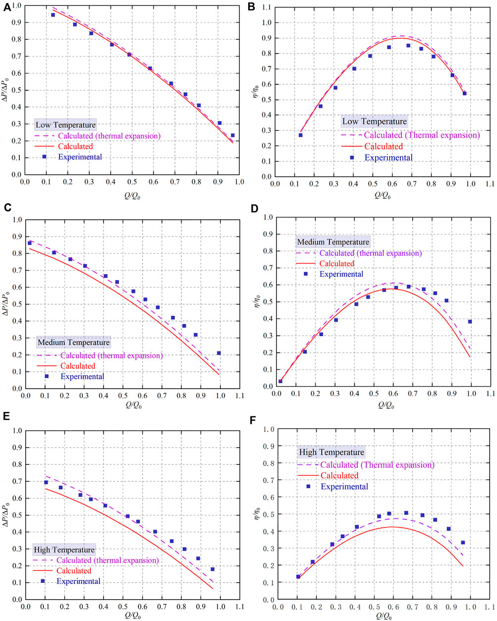
Figure 11. Comparison of the calculated and experimental values of the equivalent circuit model at different temperatures. (A) ΔP-Q (Low temperature), (B) η-Q (Low temperature), (C) ΔP-Q (Medium temperature), (D) η-Q (Medium temperature), (E) ΔP-Q (High temperature) (F) η-Q (High temperature).

From Figure 11, without considering thermal expansion, the calculated results of the analytical model head are basically consistent with the experimental data at low temperature, and the error level of the head increases significantly with the increase of temperature. After considering the thermal expansion, the average error of head is 4.78% and the average error of efficiency is 6.91% at low temperature. At medium temperature, the average error of head is 10.82% and the average error of efficiency is 12.13%. At high temperature, the average error of head is 10.36%, and the average error of efficiency is 7.95%.

The calculated results of the head and efficiency of the equivalent circuit model considering thermal expansion are in good agreement with the experimental values, and the accuracy is higher at low temperatures. In addition, the energy conversion efficiency of FLIP may deteriorate when the operating temperature is high. This may mean that FLIP is more suitable for operation at relatively low temperatures on the premise that the liquid metal does not undergo phase transition. In general, the equivalent circuit model considering thermal expansion can accurately predict the working performance of FLIP at different operating temperatures.

5 Conclusion

Based on the mathematical analysis of the two end effects, the magnetic fields of FLIP considering the influence of two end effects are analyzed, respectively. Furthermore, the performance of FLIP is calculated when the longitudinal and transverse end effects are considered separately. It is found that the analytical model considering only one type of end effect cannot accurately calculate the head and energy conversion efficiency. In view of this point, an equivalent circuit model of FLIP is proposed to comprehensively consider the longitudinal and transverse end effects. Finally, the calculated results under different voltages and operating temperatures are compared with the experimental data to validate the accuracy of the equivalent circuit model. The conclusions obtained in this paper are summarized as follows.

1) The magnetic field will be distorted due to the longitudinal and transverse end effects, which will reduce the head and energy conversion efficiency of FLIP. The performance of FLIP cannot be accurately calculated by only considering the influence of one end effect.

2) The calculated results of the established equivalent circuit model at different voltages are in good agreement with the open experimental data. The average error of head is 5.38%, and the average error of energy conversion efficiency is 7.91%.

3) When thermal effects are not considered, the calculated results of the equivalent circuit model at high temperature are significantly lower than the experimental values. After considering the thermal expansion of the core, the average error of the head under three temperature conditions is 8.65%, and the average error of the energy conversion efficiency is 9.80%. This indicates that the equivalent circuit model after considering the thermal effect can accurately calculate the performance of FLIP at different operating temperatures.

Data availability statement

The original contributions presented in the study are included in the article/Supplementary Material, further inquiries can be directed to the corresponding author.

Author contributions

MD: Funding acquisition, Methodology, Writing–original draft, Writing–review and editing. CY: Conceptualization, Data curation, Software, Writing–review and editing. YB: Conceptualization, Data curation, Software, Writing–review and editing. KB: Project administration, Resources, Writing–review and editing. XY: Supervision, Visualization, Writing–review and editing.

Funding

The author(s) declare that no financial support was received for the research, authorship, and/or publication of this article.

Conflict of interest

The authors declare that the research was conducted in the absence of any commercial or financial relationships that could be construed as a potential conflict of interest.

The author(s) declared that they were an editorial board member of Frontiers, at the time of submission. This had no impact on the peer review process and the final decision

Generative AI statement

The author(s) declare that no Generative AI was used in the creation of this manuscript.

Publisher’s note

All claims expressed in this article are solely those of the authors and do not necessarily represent those of their affiliated organizations, or those of the publisher, the editors and the reviewers. Any product that may be evaluated in this article, or claim that may be made by its manufacturer, is not guaranteed or endorsed by the publisher.

Supplementary material

The Supplementary Material for this article can be found online at: https://www.frontiersin.org/articles/10.3389/fnuen.2025.1503618/full#supplementary-material

References

Amiri, E., and Mendrela, E. A. (2014). A novel equivalent circuit model of linear induction motors considering static and dynamic end effects. IEEE Trans. Magnetics 50 (3), 120–128. doi:10.1109/TMAG.2013.2285222

CrossRef Full Text | Google Scholar

Baker, R. S., and Tessier, M. J. (1987). Handbook of electromagnetic pump technology. Elsevier.

Google Scholar

Bluhm, D. D., Fisher, R. W., and Nilsson, J. (1964). Design and operation of a flat linear induction pump. Report. doi:10.2172/4677859

CrossRef Full Text | Google Scholar

Dong, C., Zhang, C., He, G., Li, D., Zhang, Z., Cong, J., et al. (2024). 3D topology optimization design of air natural convection heat transfer fins. Nucl. Eng. Des. 429, 113623. doi:10.1016/j.nucengdes.2024.113623

CrossRef Full Text | Google Scholar

Dong, X., Mi, G., He, L., and Li, P. (2013). 3D simulation of plane induction electromagnetic pump for the supply of liquid Al–Si alloys during casting. J. Mater. Process. Technol. 213(8), 1426–1432. doi:10.1016/j.jmatprotec.2013.03.006

CrossRef Full Text | Google Scholar

Dronnik, L. M., Reutskij, S. Y., and Ehl'Kin, A. I. (1979). Simultaneous calculation of the transverse and longitudinal fringe effects in the channel of a plane induction-type MHD pump. Magnetohydrodynamics 1979 (3), 69–70.

Google Scholar

Duncan, and J. (1983). “Linear induction motor-equivalent-circuit model,” in Electric power applications iee proceedings B.

Google Scholar

Fang, X., Xu, Y., and Zhou, Z. (2011). New correlations of single-phase friction factor for turbulent pipe flow and evaluation of existing single-phase friction factor correlations. Nucl. Eng. Des. 241(3), 897–902. doi:10.1016/j.nucengdes.2010.12.019

CrossRef Full Text | Google Scholar

Gnanasekaran, T. (2022). Thermophysical and nuclear properties of liquid metal coolants. Science and Technology of Liquid Metal Coolants in Nuclear Engineering 1–101. doi:10.1016/B978-0-323-95145-6.00003-2

CrossRef Full Text | Google Scholar

Hafsi, Z. (2021). Accurate explicit analytical solution for Colebrook-White equation. Mech. Res. Commun. 111, 103646. doi:10.1016/j.mechrescom.2020.103646

CrossRef Full Text | Google Scholar

Hasani, M., and Irani Rahaghi, M. (2022). The optimization of an electromagnetic vibration energy harvester based on developed electromagnetic damping models. Energy Convers. Manag. 254, 115271. doi:10.1016/j.enconman.2022.115271

CrossRef Full Text | Google Scholar

Hou, Y., Chen, T., Li, W., Gao, C., Chen, B., Zhang, C., et al. (2024). Numerical study on surface corrosion deposition of fuel elements and its influence on flow heat transfer. Ann. Nucl. Energy 201, 110458. doi:10.1016/j.anucene.2024.110458

CrossRef Full Text | Google Scholar

Hou, Y., Sun, H., Li, J., Zhang, C., Gao, C., Chen, B., et al. (2025). Numerical study of heat transfer and pressure drop characteristics in helical tubes based on OpenFOAM. Ann. Nucl. Energy 210, 110889. doi:10.1016/j.anucene.2024.110889

CrossRef Full Text | Google Scholar

Kahourzade, S., Mahmoudi, A., Roshandel, E., and Cao, Z. (2021). Optimal design of Axial-Flux Induction Motors based on an improved analytical model. Energy 237, 121552. doi:10.1016/j.energy.2021.121552

CrossRef Full Text | Google Scholar

Kortas, I., Sakly, A., and Mimouni, M. F. (2015). Analytical solution of optimized energy consumption of Double Star Induction Motor operating in transient regime using a Hamilton–Jacobi–Bellman equation. Energy 89, 55–64. doi:10.1016/j.energy.2015.07.035

CrossRef Full Text | Google Scholar

Ku, Y. H. (1985). Electric machinery: A. E. Fitzgerald, charles kingsley, jr. and stephen D. Umans. 571 pages, diagrams, illustr. New York: McGraw-Hill Book Company. doi:10.1016/0016-0032(85)90014-6

CrossRef Full Text | Google Scholar

Liu, H. J. Y. Y. Y., Zhou, J. M., and Zhang, Z. Y. (2023). Calculation of electromagnetic characteristics of planar induction electromagnetic pump with conductive tube wall. Spec. Electr. Mach. 51 (08), 1–8. doi:10.20026/j.cnki.ssemj.2023.0099

CrossRef Full Text | Google Scholar

Lo Pinto, E., Defrasne, P., Rey, F., Talluau, M., and Verdelli, C. (2023). Performance evaluation of a high flow rate annular linear induction pump using a simple equivalent circuit model taking into account dynamic end effects. Ann. Nucl. Energy 194, 110121. doi:10.1016/j.anucene.2023.110121

CrossRef Full Text | Google Scholar

Lu, J. Y., Ma, W. M., and Li, L. R. (2008). Research on longitudinal end effect of high speed long primary double-sided linear induction motor. Lin. Ind. Mo. 28, 73–78.

Google Scholar

Naderi, P., Heidary, M., and Vahedi, M. (2020). Performance analysis of ladder-secondary-linear induction motor with two different secondary types using Magnetic Equivalent Circuit. ISA Trans. 103, 355–365. doi:10.1016/j.isatra.2020.03.013

PubMed Abstract | CrossRef Full Text | Google Scholar

Qiu, J. (1964). Liquid metal electromagnetic pump. Beijing: China Science Publishing and Media Ltd.

Google Scholar

Rao, J. S., and Sankar, H. (2011). Numerical simulation of MHD effects on convective heat transfer characteristics of flow of liquid metal in annular tube. Fusion Eng. Des. 86(2), 183–191. doi:10.1016/j.fusengdes.2010.11.009

CrossRef Full Text | Google Scholar

Sharma, P., Krishnakumar, S., Chandramouli, S., Nashine, B. K., and Mani, A. (2019). Performance evaluation of a low flow rate annular linear induction pump. Ann. Nucl. Energy 132, 299–310. doi:10.1016/j.anucene.2019.04.045

CrossRef Full Text | Google Scholar

Smolyanov, I. A., and Karban, P. (2018). “Optimal design of MHD pump,” in 2018 ELEKTRO, Mikulov, Czech Republic, 2018, 1–4. doi:10.1109/ELEKTRO.2018.8398325

CrossRef Full Text | Google Scholar

Uskov, I. A., Shvidkiy, E. L., Sarapulov, S. F., Bychkov, S. A., and Tarasov, F. E. (2016). “Induction MHD-pump with single-plane concentric winding,” in 2016 IEEE NW Russia Young Researchers in Electrical and Electronic Engineering Conference (EIConRusNW), 2-3 Feb. 2016, 723–728. doi:10.1109/eiconrusnw.2016.7448283

CrossRef Full Text | Google Scholar

Wang, L., Hou, Y., Shi, L., Wu, Y., Tian, W., Song, D., et al. (2019). Experimental study and optimized design on electromagnetic pump for liquid sodium. Ann. Nucl. Energy 124, 426–440. doi:10.1016/j.anucene.2018.10.015

CrossRef Full Text | Google Scholar

Wang, X., Wang, T., Lv, H., Wang, H., and Zeng, F. (2024). Analytical modeling and experimental verification of a multi-DOF spherical pendulum electromagnetic energy harvester. Energy 286, 129428. doi:10.1016/j.energy.2023.129428

CrossRef Full Text | Google Scholar

Zhang, F., Duan, X., Zhang, J., Ren, Q., Wu, Y., Li, Q., et al. (2024). Filtration performance and hydraulic characteristic analysis on the bottom nozzle in a fuel assembly of a nuclear energy system. Phys. Fluids 36. doi:10.1063/5.0238069

CrossRef Full Text | Google Scholar

Zhang, K., Wang, Y., Tang, H., Li, Y., Wang, B., York, T. M., et al. (2020). Two-dimensional analytical investigation into energy conversion and efficiency maximization of magnetohydrodynamic swirling flow actuators. Energy 209, 118479. doi:10.1016/j.energy.2020.118479

CrossRef Full Text | Google Scholar

Zhang, Z., Liu, H., Song, T., Zhang, Q., Yang, L., and Bi, K. (2022). One dimensional analytical model considering end effects for analysis of electromagnetic pressure characteristics of annular linear induction electromagnetic pump. Ann. Nucl. Energy 165, 108766. doi:10.1016/j.anucene.2021.108766

CrossRef Full Text | Google Scholar

Zhao, R., Dou, X., Huang, J., Zhang, D., Xia, D., and Zhang, X. (2022). Mechanisms of energy conversion in induction magnetohydrodynamic pumps for transporting conducting liquids. Energy 244, 123157. doi:10.1016/j.energy.2022.123157

CrossRef Full Text | Google Scholar