Inverse prediction of PuO2 processing conditions using Bayesian seemingly unrelated regression with functional data

Over the past decade, a variety of innovative methodologies have been developed to better characterize the relationships between processing conditions and the physical, morphological, and chemical features of special nuclear material (SNM). Different processing conditions generate SNM products with different features, which are known as “signatures” because they are indicative of the processing conditions used to produce the material. These signatures can potentially allow a forensic analyst to determine which processes were used to produce the SNM and make inferences about where the material originated. This article investigates a statistical technique for relating processing conditions to the morphological features of PuO₂ particles. We develop a Bayesian implementation of seemingly unrelated regression (SUR) to inverse-predict unknown PuO₂ processing conditions from known PuO₂ features. Model results from simulated data demonstrate the usefulness of the technique. Applied to empirical data from a bench-scale experiment specifically designed with inverse prediction in mind, our model successfully predicts nitric acid concentration, while results for Pu concentration and precipitation temperature were equivalent to a simple mean model. Our technique compliments other recent methodologies developed for forensic analysis of nuclear material and can be generalized across the field of chemometrics for application to other materials.

1 Introduction

The U.S. government is interested in the research and development of nuclear forensic techniques to identify the relationships between processing conditions and the physical, morphological, and chemical features of special nuclear material (SNM). Different processing conditions produce final SNM products with different features, which are known as “signatures” because they are indicative of the processes used to produce the material. These signatures can potentially allow a forensic analyst to determine which processes were used to produce the SNM and, as a result, make inferences about where the material originated.

Scientists at Pacific Northwest National Laboratory (PNNL) conducted an experiment designed to replicate historical and modern Pu processing methodologies and conditions. The experiment consisted of 76 runs of precipitation of Pu(III) oxalate followed by calcination to PuO₂ using the same set of seven processing parameters (e.g., temperature, nitric acid concentration, Pu concentration, etc.) whose values varied from run to run. For each run, the resulting product was imaged with a scanning electron microscope (SEM), and images were processed using the Morphological Analysis for Material Attribution (MAMA) software developed at Los Alamos National Laboratory (LANL) (Gaschen et al., 2016). The MAMA software generated measurements based on the morphological features of the particles, including particle areas, aspect ratios, convexities, circularities, gradients, and shadings (Gaschen et al., 2016). The 76-run experiment was statistically designed with inverse prediction in mind (Anderson-Cook et al., 2015), and MAMA measurements from source SEM images were captured with a consistent protocol.

In the context of nuclear forensics, inverse prediction involves predicting unknown process conditions from known PuO₂ particle features. The term “inverse” applies to the prediction of unknown values of independent variables that produced an observed, dependent response. This is contrary to standard regression techniques that predict unknown response values from known values of predictor variables (Ries et al., 2023). Lewis et al. (2018) compared multiple models for inverse prediction applied to nuclear forensics. These models all considered scaler data and sometimes targeted summary statistics for modeling, thereby losing important information contained in the whole dataset. Ries et al. (2019) converted the many particle measurements from SEM images to cumulative distribution functions and used these to discriminate among processing conditions, effectively exploiting the information in distributional measurements to improve results. Ries et al. (2023) formalized this process into a functional inverse prediction (FIP) framework that was then applied to a full bench-scale PuO₂ experiment, while Ausdemore et al. (2022) inverse-predicted PuO₂ processing conditions using Bayesian MARS techniques (Francom et al., 2018).

This article investigates a statistical technique that can be used to relate processing conditions to the morphological features of PuO₂ particles using the FIP framework from Ries et al. (2023). Specifically, we develop a Bayesian implementation of seemingly unrelated regression (SUR) to solve the inverse prediction problem in which unknown processing conditions are inverse-predicted from known PuO₂ features. The SUR methodology was developed to capture correlations among dependent variables that cannot be accommodated when each variable is modeled independently (Srivastava and Giles, 1987). This model allows different particle features from a specific experimental run to be related even after accounting for the effects of processing conditions. Embedding SUR in a Bayesian framework allows us to quantify the uncertainty in the inverse predictions because Bayesian analysis returns an entire distribution rather than simply a point estimate. In Section 2, we outline the inverse prediction problem and provide details on the modeling framework employed in this study. In Section 3, we apply the statistical methodology to both a simulated dataset and the empirical PuO₂ dataset obtained from PNNL, and in Section 4 we summarize our conclusions.

2 Modeling framework

2.1 Inverse prediction

To study the relationship between independent variables (i.e., predictor variables such as PuO₂ processing conditions) and dependent variables (i.e., response variables such as PuO₂ particle features), we apply an inverse prediction framework (Ries et al., 2023). Consider an observation y of a dependent variable and a p-dimensional input vector $\mathit{x}={(x_1,x_2,\dots ,x_p)}^{\prime }$ of independent variables. We express the relationship between x and y as y = g(x|θ) + ϵ, where g(⋅) is the true underlying physical process that is responsible for producing the observation, θ is a vector of model parameters, and ϵ is a random variable that captures noise present in the observed data.

The goal of the inverse prediction framework is to predict the values of the independent variables x′ that produced a new observation y′. There are two approaches by which we can learn about x′: (1) construct an inverse model that directly predicts x′ as a function of y′ or (2) invert a traditional forward model that predicts y′ as a function of x′. Under approach (1), we reframe the model representation as x′ = h(y′|ϕ) + δ, where ϕ is a vector of parameters associated with h(⋅), and δ is a random error term. This approach violates traditional regression assumptions, however, as regression models assume that the independent variable is measured with negligible error, and it is the dependent variable that is associated with some error (Poole and O’Farrell, 1971).

The assumption that the independent variables are measured without error is unrealistic (e.g., processing conditions can only be measured to the accuracy of the measuring device), and complex processes require a more sensible model. Approach (2) involves reconstructing the model as x′ = g⁻¹(y′|θ) + τ, where τ is a mean-zero random error term capturing the measurement error associated with the independent variables. Inverse problems analyzed in this way are sometimes ill-posed in the sense that a classical least squares, minimum distance, or maximum likelihood solution may not be uniquely defined. For example, if g(⋅) is of the form β₀ + β₁x′, x′ is given by $\frac{y^{\prime }-{\beta }_0}{{\beta }_1}$. The case where β₁ = 0 is clearly ill-posed, but even if β₁ does not exactly equal zero, values close to zero can produce estimates for x′ that are highly unstable: large perturbations of y′ can lead to very small changes in the estimate for x′, and vice versa (O’Sullivan, 1986; Osborne, 1991).

More generally, an inverse problem is ill-posed if more than one set of independent variables produces statistically indistinguishable observed values of the dependent variable (i.e., any difference in observed values from x and x′, x ≠ x′ is smaller than the noise). As discussed in the introduction, the goal of the PuO₂ bench-scale experiment is to detect production signatures in which different process characteristics produce identifiably different particle features, and the underlying assumption is that these signatures exist. The goal of this study is to solve the inverse problem in which we predict the unknown values of the independent variables (PuO₂ processing conditions) from observed values of the dependent variables (PuO₂ particle features). A successful application of our technique to the bench-scale experiment suggests that the inverse problem is not ill-posed and that such signatures do exist and are detectable.

2.2 Functional data analysis

Functional data analysis (FDA) is the branch of statistics concerned with continuous data, such as curves and surfaces, that naturally present themselves as functions of time, frequency, location, or some other index (Ramsay, 2005; Srivastava and Klassen, 2016). Analyses of functional data based on summary statistics do not make use of important information such as correlations contained in the smoothness of the curve. FDA techniques consider the curve as one functional measurement, where information is contained in the curve as a whole rather than at individual sample points.

Here we employ the FIP framework described in Ries et al. (2023), and assume the observed values of the dependent variables are generated by an underlying continuous process that can be expressed in functional form. The general strategy is to represent the discrete dependent-variable data in functional form using basis functions and then use the discrete values of the basis functions in the model computations. We use the data from the bench-scale experiment described in Section 3.2 below to illustrate the procedure.

MAMA processing of the bench-scale experiment data produced observations on a variety of PuO₂ particle features such as circularity and greyscale mean. We model a subset of four features produced in 24 experimental runs (see Section 3.2 below for a full description of the bench-scale data). FDA models the particle features as smooth functions of the processing conditions. We begin with y_ija, a single observation from particle a, a = 1, … , n_i of particle feature j, j = 1, … , 4 from experimental run i, i = 1, … , 24. The vector y_ij is an n_i-vector of observations of feature j from run i, which can be ordered as ${\mathit{y}}_{ij}^{\prime }=(y_{ij[1]},y_{ij[2]},\dots ,y_{ij[n_i]})$, where [a] indicates the a^th order statistic (i.e., y_ij[1] is the lowest value, y_ij[2] is the second-lowest, and $y_{ij[n_i]}$ is the highest value in the vector of observations). We compute the empirical cumulative probabilities associated with each y_ija as $\frac{[a]}{n_i}$. The set of all possible values for the particle feature is its (infinite) functional domain T, and the empirical cumulative distribution function (eCDF) is:

${\widehat{F}}_{ij}\left(t\right)=\frac{1}{n_i}{\displaystyle \sum _{a=1}^{n_i}}I\left(Y_{\mathit{ija}}<t\right)$

The eCDF is a monotonically increasing function that assigns a probability to every value in the domain T, specifically the probability that an observation will be less than or equal to the value t.

Conceptually, the next step in FDA is to consider ${\widehat{F}}_{ij}(t)$ as an observed estimate of the true function F_ij(t) that represents the true, smooth CDF of particle feature j. F_ij(t) can be represented as a sum of basis functions:

$F_{ij}\left(t\right)={\displaystyle \sum _{l=1}^{\infty }}{\zeta }_l{\varphi }_l\left(t\right)\approx {\displaystyle \sum _{l=1}^m}{\zeta }_l{\varphi }_l\left(t\right)$

where Φ is an infinite matrix of basis vectors with m rows that contain the values of the m basis functions ϕ_l(t) evaluated across the infinite domain T. The m-vector ζ contains the coefficients on the basis functions. This vector is what we model because if we apply $\widehat{\mathit{\zeta }}$ back to the matrix of basis vectors Φ, we produce an estimate of our original function F_ij(t).

The description above outlines the conceptual steps involved in FDA, however computationally the basis representation of F_ij(t) must be calculated over a discrete number of values for t. To accomplish this, we calculate a finite (large) number of quantile values from the eCDF ${\widehat{F}}_{ij}(t)$, concatenate the runs i into a matrix Z_j, and apply a basis decomposition to this matrix of quantiles. For our study, we calculated 100 quantiles (n_t = 100) from each of the 24 eCDFs (one eCDF per run) associated with particle feature j, resulting in a 24 × 100 matrix Z_j. The matrix Z_j is an approximation of the functional space that characterizes the relationship between processing conditions and particle characteristic j; our 24 experimental runs are statistical samples from this functional space.

Functional data analysis applications commonly use functional principal component analysis (fPCA) for the basis representation of F_ij(t). To compute the fPCA, we define a sample covariance operator for the functions F(t) as

$K=\frac{1}{n-1}{\displaystyle \sum _{i=1}^n}\left(F_{ij}-{\mu }_{F_j}\right){\left(F_{ij}-{\mu }_{F_j}\right)}^{\mathsf{T}}\in {\mathbb{R}}^{T\times T}\text{,}$

where ${\mu }_{F_j}$ is the functional mean. Taking the eigen decomposition in functional space, $K=V\mathrm{\Psi }{V}^{\mathsf{T}}$, we calculate the directions of principle variability using the first p ≤ n columns of V. For computational purposes, we perform fPCA using an eigen decomposition of a discretized version of the functions (that is, we perform PCA on Z_j).

${\mathit{Z}}_j\stackrel{fPCA}{\to }{\mathit{Z}}_j^{\prime }\approx {\mu }_F+{\displaystyle \sum _{l=1}^m}{\mathit{s}}_{jl}{\mathit{v}}_{jl}={\mu }_F+{\mathit{S}}_j{\mathit{V}}_j^{\mathsf{T}}$

Here, m = 24 and the 24 × 100 matrix ${\mathit{V}}_j^{\mathsf{T}}$ is the matrix of eigenvectors of Z_j that contain the discrete approximations of the eigenfunctions of F_ij(t). The 24 × 24 matrix S_j contains the principal component scores $\mathit{s}=⟨(F_i-{\mu }_F),{\mathit{V}}_j⟩$ associated with ${\mathit{V}}_j^{\mathsf{T}}$. The matrix ${\mathit{Z}}_j^{\prime }$ is an approximation of F_ij(t), which represents the functional space characterizing the relationship between the processing conditions and particle feature j. We model the principal component scores in S_j, and when we apply the model estimates ${\widehat{\mathit{S}}}_j$ back to V_j we recover our original functional space represented by F_ij(t). With these estimates in hand, we are able to inverse-predict the values of the processing conditions.

Rather than modeling our original n_i-element vector y_ij of observations, we instead model 24-element vectors of principal component scores s_jl. The matrix S_j captures information about the entire functional space because it is calculated from the matrix Z_j, which contains information from all 24 samples from the functional space. Furthermore, the FDA approach accounts for correlations along the functional domain. By using fPCA for the basis decomposition, we are able to model a small subset of the vectors in S_j, because fPCA is designed to capture a large portion of the variability in the data in the first few principal components. Ries et al. (2023) demonstrate the improvements to prediction results that can be achieved using FDA techniques on data that is functional versus treating that data as an independent collection of scalar values.

2.3 Seemingly unrelated regression

Seemingly unrelated regression is a generalization of linear regression involving several univariate regression equations, each having its own dependent variable, potentially different sets of independent variables, and potentially different relationships between dependent and independent variables (Srivastava and Giles, 1987). Each model equation is a valid linear regression on its own and could be estimated separately, but in SUR the error terms are allowed to be correlated across equations. SUR was developed for scalar rather than functional data, and we follow that development here; at the end of this section, we extend the SUR model to functional data. If there are n observations in each of k vectors of dependent variables, y_iq, i = 1, … , n; q = i, … , k is a single observation i of dependent variable q. We apply the SUR model to an n × k matrix of dependent variable values, and each regression equation q takes the form:

${\mathit{y}}_q={\mathit{X}}_q{\mathit{\beta }}_q+{\mathit{ϵ}}_q,{ϵ}_{iq}\perp {ϵ}_{jq}\text{\hspace{0.17em}for\hspace{0.17em}}i\ne j$

where y_q is an n × 1 vector of dependent variable values, ϵ_q is an n × 1 vector of independent error terms, X_q is an n × p_q matrix, where p_q is the number of independent variables for regression equation q, and β_q is a p_q × 1 vector of regression coefficients specific to regression equation q. Stacking the k vectors yields:

$\left(\begin{array}{c}\hfill {\mathit{y}}_1\hfill \\ \hfill {\mathit{y}}_2\hfill \\ \hfill ⋮\hfill \\ \hfill {\mathit{y}}_k\hfill \end{array}\right)=\left(\begin{array}{cccc}\hfill {\mathit{X}}_1\hfill & \hfill 0\hfill & \hfill \dots \hfill & \hfill 0\hfill \\ \hfill 0\hfill & \hfill {\mathit{X}}_2\hfill & \hfill \dots \hfill & \hfill 0\hfill \\ \hfill ⋮\hfill & \hfill ⋮\hfill & \hfill \ddots \hfill & \hfill ⋮\hfill \\ \hfill 0\hfill & \hfill 0\hfill & \hfill \dots \hfill & \hfill {\mathit{X}}_k\hfill \end{array}\right)\left(\begin{array}{c}\hfill {\mathit{\beta }}_1\hfill \\ \hfill {\mathit{\beta }}_2\hfill \\ \hfill ⋮\hfill \\ \hfill {\mathit{\beta }}_k\hfill \end{array}\right)+\left(\begin{array}{c}\hfill {\mathit{ϵ}}_1\hfill \\ \hfill {\mathit{ϵ}}_2\hfill \\ \hfill ⋮\hfill \\ \hfill {\mathit{ϵ}}_k\hfill \end{array}\right)(1)$

For a given dependent variable vector y_q the observations y_iq and y_jq are assumed to be independent (cov(y_iq, y_jq) = 0, i ≠ j) but we allow for cross-response correlations between y_q and y_r (cov(y_iq, y_ir) = σ_qr ≠ 0). The nk × 1 vector ϵ is assumed to be distributed multivariate normal (MVN) with mean 0 and covariance matrix Ω, where Ω has the form Σ ⊗I_n, and Σ is the k × k skedasticity matrix containing the correlations between y_iq and y_ir: σ_qr at row q and column r of Σ.

The preceding development describes the SUR modeling framework for the case when the response variables are scalars rather than functions. When the dependent variables are scalars, allowing for correlated errors across regression functions allows us to appropriately model situations in which the dependent variables are correlated beyond what the independent variables can capture. That is, after removing the effects of the processing conditions, there is still residual information relating to the measurements of the particle features. The computational steps are the same for scalar and functional data analysis, but the interpretation is different for FDA. In the functional case, the dependent variables are the basis coefficients (which can be converted back to functional space using their respective basis functions, as described in Section 2.2). The correlated error terms represent the difference between the functional response (i.e., the CDF of the particle feature values) and what can be explained by the smooth variation in the processing conditions. This model allows the residual functions for an experimental run i, ϵ_i1(t) and ϵ_i2(t), to be related even after removing the effects of the independent variables. It is important to allow for these correlations in our study because all the particles in a run are measurements from the same experimental setup, or batch, which involves not only the run-specific effects of the processing conditions but also run-specific effects of the environment, operator, etc. The residual correlation is related to the effect of the run.

The vector β = (β₁, β₂, … , β_k)^T, the unknown values of the processing conditions, and the skedasticity matrix Σ were estimated using Bayesian Markov chain Monte Carlo (MCMC) methods, which produce an approximation to a posterior distribution of interest through repeated sampling. Because Bayesian analysis returns an entire distribution for each inverse prediction, we are able to quantify the uncertainty in the prediction by examining the variance of the posterior predictive distribution. We placed uninformative Normal priors on the βs (β ∼ N(0, 100)) and on the unknown processing condition values (x ∼ N(0, 100)). The prior on the Σ matrix was an uninformative Wishart distribution, the conjugate prior of the MVN, with degrees of freedom equal to k and a scale matrix equal to the k × k identity matrix. Models were run using 4 independent MCMC chains in the R package rjags, which calls the C++ program JAGS to implement a Gibbs MCMC sampling algorithm (R Core Team, 2021; Plummer, 2022; Plummer et al., 2003). Chains were initialized with 1 million iterations (sampler adaptation) and updated with 1 million iterations (burn-in), then sampled 100,000 times and thinned every 100 steps. We monitored the convergence of the MCMC chains to a stationary distribution using trace plots and the Gelman-Rubin diagnostic statistic (Gelman and Rubin, 1992).

3 Applications

In this section, we synthesize the FDA and SUR techniques under a Bayesian framework to inverse-predict synthetic and empirical data sets. We consider first a synthetic dataset in which dependent variable values are generated deterministically, without added stochastic error, then the same dataset with the addition of stochastic error to the dependent variable values. Finally, we apply the functional SUR methodology to empirical data generated by the PNNL bench-scale experiment.

3.1 Simulated data

3.1.1 Methods

To test the feasibility of the model, we simulated data using two independent variables, x₁ and x₂, and two functional dependent variables, y₁(t) and y₂(t), over the functional domain T. We chose 20 evenly-spaced values each for x₁ and x₂ on the ranges specified below, then created 20 pairs (x_1i, x_2i), i = 1, … , 20 and evaluated each function y₁(t) and y₂(t) for each (x₁, x₂) at 150 evenly-spaced values on the domain T.

$\begin{array}{cc}\hfill t& \in \left[-\mathrm{4,4}\right]\hfill \\ \hfill x_1& \in \left[0.5,2.4\right]\hfill \\ \hfill x_2& \in \left[0.1,2\right]\hfill \\ \hfill y_1\left(t\right)& =\frac{1}{x_1\sqrt{2\pi }}{\int }_{-\infty }^t\exp \left\{-\frac{1}{2}{\left(\frac{t}{x_1}\right)}^2\right\}dt\hfill \\ \hfill y_2\left(t\right)& =x_1\sin \left(x_{2}t\right)\hfill \end{array}$

Figures 1A, B display the dependent variables y₁(t) and y₂(t) as functions of (x₁, x₂) over the domain t. After applying fPCA to the raw functional response values, we used principal component scores from the first three principal components (PCs) of y₁(t) and y₂(t) to create a total of six dependent variables. Recall that in FDA an “observation” is a single functional measurement; here n = 20 since each curve generated by the 20 (x₁, x₂) pairs is one “observation,” and each dependent variable is a vector of 20 elements (principal component scores). As described in Section 2.3 above, each of the six regression equations in the SUR model (one regression equation for each dependent variable) takes the form y_q = X_qβ_q + ϵ_q, q = 1, … , 6. We estimate the coefficient vector β_q and the 6 × 6 skedasticity matrix Σ containing the σ_qr correlations across regression equations.

Figure 1

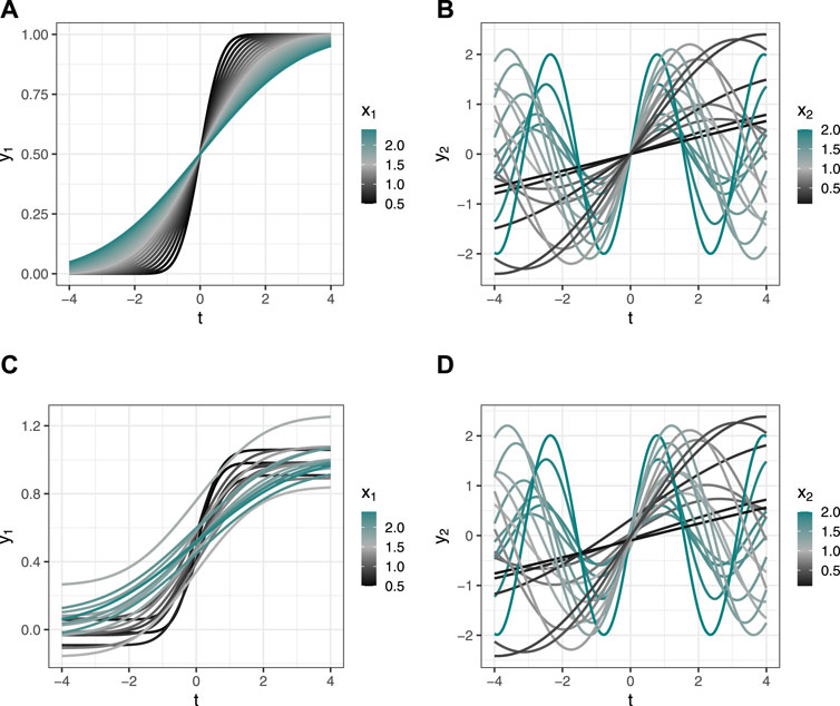
Figure 1. Simulated data. (A,B) Data simulated without added error; y values are deterministic. (C,D) Data simulated with stochastic error added to y values. (A,C) Variable y₁(t) as a function of x₁ over the domain t. (B,D) Variable y₂(t) as a function of (x₁, x₂) over the domain t. Value for x₁ not shown.

We first tested the technique in a simplified situation in which the dependent variables are “observed” without error: six vectors of principal component scores calculated from the deterministic values of y₁(t) and y₂(t). To these dependent variables, we applied four models that an analyst might reasonably be expected to try on these data.

• Base Model: ${\mathit{y}}_q={\beta }_{0_q}+{\beta }_{1_q}{\mathit{x}}_1+{\beta }_{2_q}{\mathit{x}}_2+{\mathit{ϵ}}_q$

• Interaction Model: ${\mathit{y}}_q={\beta }_{0_q}+{\beta }_{1_q}{\mathit{x}}_1+{\beta }_{2_q}{\mathit{x}}_2+{\beta }_{3_q}{\mathit{x}}_1{\mathit{x}}_2+{\mathit{ϵ}}_q$

• Quadratic Model: ${\mathit{y}}_q={\beta }_{0_q}+{\beta }_{1_q}{\mathit{x}}_1+{\beta }_{2_q}{\mathit{x}}_2+{\beta }_{3_q}{\mathit{x}}_1^2+{\beta }_{4_q}{\mathit{x}}_2^2+{\mathit{ϵ}}_q$

• Sine model: ${\mathit{y}}_q={\beta }_{0_q}+{\beta }_{1_q}{\mathit{x}}_1+{\beta }_{2_q}{\mathit{x}}_2+{\beta }_{3_q}{\mathit{x}}_1^2+{\beta }_{4_q}\sin ({\mathit{x}}_2)+{\mathit{ϵ}}_q$

Once we demonstrated the SUR technique on functional data without error, we simulated errors and added the simulated error values across the domain T. That is, we assumed that the error was constant across the functional domain. Raw response values for y₁(t) and y₂(t) ranged between 0 and 1 with a mean and median of 0.5. Error vectors ${\mathit{\delta }}_{y_1}$ and ${\mathit{\delta }}_{y_2}$ were simulated using a MVN distribution with a mean of 0, a variance of 1 for each y variable, and a covariance of 0.9 between ${\mathit{\delta }}_{y_1}$ and ${\mathit{\delta }}_{y_2}$. After generating the δ values and multiplying by 0.1 to scale them appropriately to the data, the measured covariance between the two error vectors was 0.886. The δ values for y₁ ranged between [−0.16, 0.26] with median −0.002, and the δ values for y₂ ranged between [−0.23, 0.32] with median −0.020. These error vectors were added to the deterministic y values prior to performing fPCA, and subsequent modeling steps were identical to those performed on the simulated data without added error. Figures 1C, D display the dependent variables y₁(t) and y₂(t) as functions of (x₁, x₂) over the domain t with added error.

We assessed the performance of each model on data both with and without added error by calculating the root mean squared error (RMSE) of the predicted values $\widehat{x}$ using leave-one-out cross-validation (LOOCV).

$RMSE\left(\widehat{\mathit{x}}\right)=\sqrt{\frac{{\sum }_{I=1}^n{\left({\widehat{x}}_i-x_i\right)}^2}{n-1}}(2)$

The LOOCV technique removes the first observation from the dataset, trains the model on the n − 1 observations, and then predicts the left-out observation using the trained model. The first observation is then replaced and the second observation removed, the model is again fit using n − 1 observations, and a prediction for the second observation is made. The process is repeated for all observations in the dataset, and the vector of predictions $\widehat{\mathit{x}}$ is then compared to the vector of true values x using Eq. 2. Because the independent variables in our datasets have been centered and scaled, an RMSE value of 1 describes the expected error associated with using the sample mean as the inverse prediction.

3.1.2 Results and discussion

Overall, the technique and specific models performed well and the prediction error was small. All models were better able to inverse-predict x₁ than x₂, and performance was better on the datasets without added error. The quadratic model performed best on both datasets, followed by the sine model (Table 1; Figure 2).

Table 1

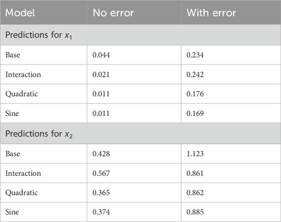
Table 1. Model assessment, simulated data. RMSE for simulated data both before and after error terms were added to the response values. RMSE = 1 indicates parity with mean-only model.

Figure 2

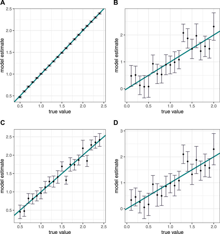
Figure 2. Simulated data results. Inverse predictions versus true values for x variables, with 95% credible interval. The plotted blue line is y = x and is used for assessment of results. (A,B) Results from data simulated without error. (C,D) Results from data simulated with error. (A,C) Inverse predictions for x₁. (B,D) Inverse predictions for x₂.

We originally ran the models using only the first two PCs of the y vectors. While this was adequate for the dataset without added error, the interaction, quadratic, and sine models did not converge on a distribution for x₂ using the dataset with added error when only two PCs were considered. Model convergence was adequate when using three PCs rather than two as determined by an examination of traceplots and the Gelman-Rubin statistic (Gelman and Rubin, 1992; Brooks and Gelman, 1998). The δ values added about 1%–30% noise to the observations. The cumulative percent of variance explained using 2 and 3 PCs for y₁ was 98.4.% and 99.9% respectively, and for y₂ was 78.6% and 94.6% respectively. These results are consistent with the general principle that more information is needed to fit noisier data and/or more complex models. Quantitatively, the basis functions for the system of equations used to generate our simulated data with the magnitude of error described above need to capture at least 95% of the observed variability in order for the more complex models to have enough information to provide reliable predictions.

Finally, we draw attention to the assumption that the error is constant across the functional domain. Computationally, this means we added the same ${\delta }_{y_{1_i}}$ value to $y_{1_i}(t)\forall t$ and the same ${\delta }_{y_{2_i}}$ value to $y_{2_i}(t)\forall t$. Empirically, this assumption corresponds to the situation in which the mean and variance of the observation error do not change over the functional domain. When the functional domain is concrete, such as time or space, it may be possible to test the validity of this stationarity assumption. For example, we can ask if a measuring instrument loses precision and/or accuracy over time. In many situations, however, including both our simulated data and the observed values of the PuO₂ particle features, the functional domain is abstract, and in these cases it will be difficult if not impossible to check the validity of the stationarity assumption. Here we simply apply the errors as described above and leave development of this topic for future work.

3.2 Benchscale experiment

3.2.1 Methods

The PNNL bench-scale experiment was a 76-run experiment that replicated historical and modern PuO₂ processing methods for processing precipitation of Pu(III) oxalate followed by calcination to PuO₂. It was statistically designed with inverse prediction in mind (Anderson-Cook et al., 2015). For this study, we analyzed a subset of the data consisting of the 24 runs that used solid oxalic acid: specifically, Pu(III) oxalate was precipitated from a plutonium nitrate solution by the addition of solid oxalic acid, while ascorbic acid and hydrazine were used to adjust the oxidation state and for stabilization. The plutonium oxalate precipitate was filtered from the mother solution and washed, followed by calcination at 650°C for 2 h. The processing conditions whose values varied over these 24 runs were plutonium nitrate concentration (“Pu concentration”), nitric acid concentration, and plutonium nitrate temperature during precipitation (“precipitation temperature”). All other processing conditions were held constant and actual values measured and recorded. Pu concentration and nitric acid concentration were each set to one of three different factor levels (i.e., three values for the processing condition), while precipitation temperature was set to one of two factor levels, for a total of 18 possible combinations of processing condition values. Six runs duplicated processing condition values already included in the 18 possible combinations, for a total of 24 experimental runs, of which 12 are duplicated runs.

The reaction equation is:

$2\mathrm{P}\mathrm{u}{\left({\mathrm{N}\mathrm{O}}_3\right)}_3+3{\mathrm{H}}_2{\mathrm{C}}_2{\mathrm{O}}_4+6{\mathrm{H}}_2\mathrm{O}\rightleftarrows {\mathrm{P}\mathrm{u}}_2{\left({\mathrm{C}}_2{\mathrm{O}}_4\right)}_3+6{\mathrm{H}}_2\mathrm{O}+6{\mathrm{H}\mathrm{N}\mathrm{O}}_3$

Plutonium nitrate concentration, nitric acid concentration, and precipitation temperature all have the potential to influence the reaction equilibrium or precipitation rate, in turn affecting the morphology of the precipitate. This impact on the plutonium oxalate morphology can carry through to influence the morphology of the PuO₂ product.

For each run, the resulting PuO₂ material was imaged with a SEM (Figure 3). The minimum number of particles imaged per run was 115 and the maximum was 831. SEM images were processed using MAMA, a publicly available software package developed by LANL to help automate the processing of SEM images of special nuclear material (Gaschen et al., 2016). After images are uploaded, the software separates the image from the background, identifies and separates different crystals if multiple crystals are included in a single image, and calculates 22 morphological characteristics per crystal from the processed data. Measuring particle characteristics begins with defining the boundary of the particle: MAMA uses several methods including a convex hull and a best-fit ellipse. Based on the particle boundary, MAMA calculates particle characteristics including area, major and minor ellipse axis lengths and their ratio, degree of circularity, and several measures of grayscale pixel intensity.

Figure 3

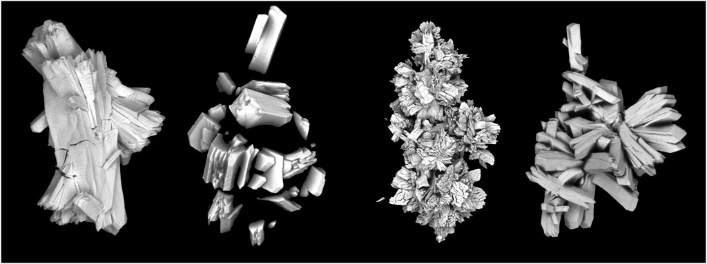
Figure 3. SEM images of PuO₂ particles.

In this study, we investigate four PuO₂ particle features: pixel area, ellipse aspect ratio, gradient mean, and area convexity. Pixel area is the area of the particle calculated by counting the total number of pixels within the object boundary and then multiplying by the micrometer/pixel scale. The ellipse aspect ratio is the ratio of the minor to the major axis of the best-fit ellipse. Gradient mean uses the Sobel operator, a differentiation operator, to calculate the gradient of the image pixel intensity values in the x and y directions, then combines them to give a single gradient magnitude value for each pixel location. The mean of these values is the gradient mean, which can serve as a measure of particle topology or texture. Although the gradient mean can be sensitive to the focus or contrast of the SEM image, we assume that the noise associated with this variability is small relative to the signal in the measurement. Finally, area convexity is a measure of the ratio of the area of the object to the convex hull area.

All measures of area are strongly correlated, as are all measurements that involve pixel intensity, etc. Each of the four particle characteristics we analyze here represents one of four groups of correlated features identified in preliminary data analysis. Correlations between pairs of variables were generally low for all runs (median absolute correlation = 0.15, Figure 4).

Figure 4

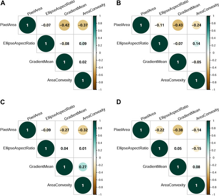
Figure 4. Selected particle feature correlations. (A) Correlations over all 24 experimental runs. (B) Correlations for experimental run 9. (C) Correlations for experimental run 15. (D) Correlations for experimental run 16.

To represent the values of the PuO₂ particle features in functional form, we first calculated eCDFs for the 24 runs for each of the four particle features (Figure 5). We then applied fPCA to the four matrices of observed values and conducted “forward-direction” variable selection on the principal component scores to determine which particle feature PCs were most relevant to a given processing condition. Here, “forward-direction” indicates that we use the particle feature PCs to predict each processing condition directly, and apply variable selection techniques to determine which PCs are important to predicting each processing condition.

Figure 5

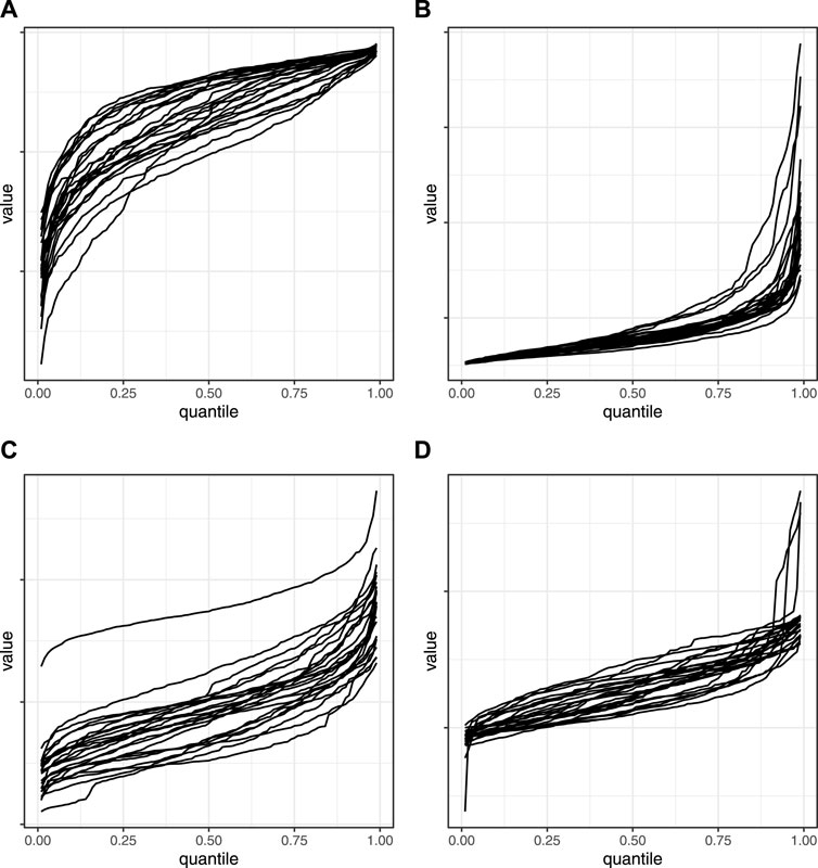
Figure 5. Empirical cumulative distribution functions. eCDFs of particle features from 24 experimental runs. (A) Area convexity. (B) Ellipse aspect ratio. (C) Gradient mean. (D) Pixel area.

The three processing conditions were modeled separately using two variable-selection techniques: stepwise regression and lasso (James et al., 2021). In stepwise regression, independent variables are incrementally added and/or subtracted to a starting intercept-only model, and model fit is assessed at each step using information criteria such as AIC or BIC. The procedure stops when the optimal model has been identified, and the predictor variables from the optimal model are selected as important for predicting the dependent variable. For stepwise regression, particle feature PCs that scored below a threshold p-value, 0.001, were considered important predictors for the modeled processing condition.

Lasso is a variable-selection technique that constrains, or regularizes, the coefficient estimates in a linear regression model, thus shrinking some coefficient estimates to zero or near zero. The independent variables with larger coefficient values are then selected as important to predicting the dependent variable. The lasso algorithm was run 20 times for each processing condition in order to ensure the stability of results, and the results were visually inspected to produce two sets of dependent variables: a larger set with more particle feature PCs and a smaller set with fewer.

For each variable selection technique, the particle feature PCs that were identified as important were combined across processing conditions into a matrix of dependent variables and an associated index matrix that identified which PCs were important for which processing conditions. The final analysis incorporated four sets of dependent variables, each modeled independently: those selected by stepwise regression, a larger set of lasso variables, a smaller set of lasso variables, and only variables that were stepwise identified as important for predicting nitric acid concentration:

• Stepwise variable selection: 16 PCs

• Lasso large: 11 PCs

• Lasso small: 5 PCs

• nitric acid concentration variables: 13 PCs

We fit four models separately to each set of variables: a simple linear model, a quadratic model, and two interaction models. As described in Section 2.3 above, each regression equation in the SUR model takes the form y_q = X_qβ_q + ϵ_q, q = 1, … , k for k regression equations associated with k dependent variables. Specifically:

• Simple linear model: y_q = β₀ + β₁x₁ + β₂x₂ + β₃x₃ + ϵ_q

• Quadratic model: ${\mathit{y}}_q={\beta }_0+{\beta }_1{\mathit{x}}_1+{\beta }_2{\mathit{x}}_2+{\beta }_3{\mathit{x}}_3+{\beta }_4{\mathit{x}}_1^2+{\beta }_5{\mathit{x}}_2^2+{\beta }_6{\mathit{x}}_3^2+{\mathit{ϵ}}_q$

• Interaction model: y_q = β₀ + β₁x₁ + β₂x₂ + β₃x₃ + β₄x₁x₂ + β₅x₁x₃ + β₆x₂x₃ + β₇x₁x₂x₃ + ϵ_q

We estimate the coefficient vector β and the k × k skedasticity matrix Σ containing the σ_qr correlations across regression equations. For the bench-scale data n = 24 for the full dataset, and n = 12 for the duplicated dataset—one observed curve for each run of the experiment.

The matrix of independent variables X_q—the values of the processing conditions to be inverse-predicted—contains only those processing conditions for which the q^th principal component was determined to be important in the variable selection step. For example, suppose y_q is a vector of principal component scores that was identified as being related to Pu concentration and nitric acid concentration in the “forward-direction” variable selection process. The models for the q^th regression equations are:

• Simple linear model: y_q = β₀ + β₁x₁ + β₂x₂ + ϵ_q

• Quadratic model: ${\mathit{y}}_q={\beta }_0+{\beta }_1{\mathit{x}}_1+{\beta }_2{\mathit{x}}_2+{\beta }_4{\mathit{x}}_1^2+{\beta }_5{\mathit{x}}_2^2+{\mathit{ϵ}}_q$

• Interaction model: y_q = β₀ + β₁x₁ + β₂x₂ + β₄x₁x₂ + ϵ_q

The terms associated with precipitation temperature are not included in these models because y_q was not identified as important to predicting precipitation temperature. If y_r is a different vector of principal component scores that was (for example) identified as being related to Pu concentration and precipitation temperature in the “forward-direction” variable selection process, the models for the r^th regression equations are:

• Simple linear model: y_q = β₀ + β₁x₁ + β₃x₃ + ϵ_q

• Quadratic model: ${\mathit{y}}_q={\beta }_0+{\beta }_1{\mathit{x}}_1+{\beta }_3{\mathit{x}}_3+{\beta }_4{\mathit{x}}_1^2+{\beta }_6{\mathit{x}}_3^2+{\mathit{ϵ}}_q$

• Interaction model: y_q = β₀ + β₁x₁ + β₃x₃ + β₅x₁x₃ + ϵ_q

Note the subscripts on the β coefficients do not change from the full models that include all independent variables to the individual regression models. (The different model forms are computed separately, so β₀ in the linear model is different from β₀ in the quadratic model, but β₀ in linear regression equation q is the same as β₀ in linear regression equation r). In the example above, the q^th linear regression equation provides no information for estimating β₃, but the r^th linear regression equation does. In the Bayesian framework, the β vector from Eq. 1 is estimated simultaneously and the complete set of k regression equations together contains information for estimating all β coefficients.

We applied the interaction model to two different sets of dependent variables. In the “sparse” interaction model, processing conditions were only included in the design matrix X_q if both (or all three) were associated with the given dependent variable y_q (an “and” requirement). In the “full” interaction model, processing conditions were included if any of them were associated with the given dependent variable (an “or” requirement).

As with the simulated data, we assessed the performance of each model by calculating RMSE using LOOCV. We also compared results from the SUR framework to those from standard regression techniques by modeling each dependent variable separately, outside of the SUR framework. That is,

${\mathit{y}}_q={\mathit{X}}_q{\mathit{\beta }}_q+{\mathit{ϵ}}_q,{ϵ}_{q_i}\sim N\left(0,{\sigma }^2\right),{\mathit{ϵ}}_{q_i}\perp {\mathit{ϵ}}_{q_j}\text{\hspace{0.17em}and\hspace{0.17em}}{\mathit{ϵ}}_{q_i}\perp {\mathit{ϵ}}_{r_i}\text{\hspace{0.17em}for\hspace{0.17em}}i\ne j\text{\hspace{0.17em}and\hspace{0.17em}}q\ne r.$

We also independently modeled the complete dataset of 24 runs as well as the smaller dataset of 12 duplicated runs, expecting predictive performance to be better for the duplicated dataset. In the duplicated dataset, each set of processing condition values appears twice. Therefore, when we leave out one observed value of the dependent variable in LOOCV, the independent variables that produced that observation are included in the modeled dataset. This is not the case for 12 observations in the full n = 24 dataset, and we expected predictions on those 12 observations to be less accurate.

3.2.2 Results and discussion

In general, the Bayesian SUR technique successfully inverse-predicted nitric acid concentration values, but other predictions performed no better than a simple mean model. The best model performance came from predicting nitric acid concentration values from a quadratic model using variables stepwise selected as important for predicting nitric acid concentration (RMSE = 0.40 for the duplicated dataset, 0.59 for the full dataset. Table 2; Figures 6, 7. See Supplementary Table S1 for full results).

Table 2

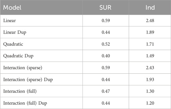
Table 2. Model assessment, benchscale data. RMSE values for inverse predictions of nitric acid concentration from the model using variables identified as important for predicting nitric acid concentration. An RMSE of 1 indicates parity with a mean-only model. “SUR” indicates results from the SUR models, while “Ind” indicates results from models run as independent regressions (outside the SUR context). “Dup” indicates the model was implemented on the dataset with 12 duplicated experimental runs, otherwise model was implemented on full 24-run dataset.

Figure 6

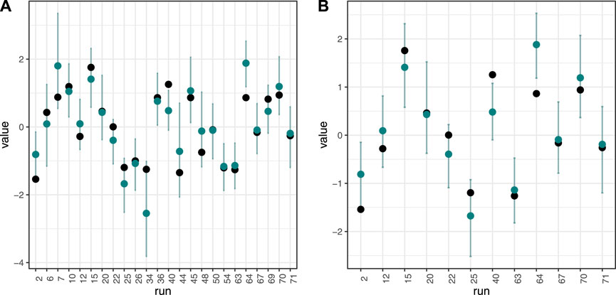
Figure 6. Model results. Inverse prediction (blue point) for nitric acid concentration, with 95% credible interval for predicted mean. Black point is true value. All models used independent variables selected as important for predicting nitric acid concentration. (A): Results from dataset using all 24 experimental runs. (B): Results from dataset using 12 duplicated experimental runs.

Figure 7

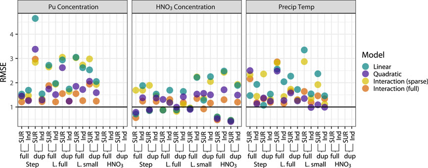
Figure 7. Model assessment, benchscale data. RMSE values for inverse predictions of all processing conditions. An RMSE of 1 indicates parity with a mean-only model. “SUR” indicates results from the SUR models, while “Ind” indicates results from models run as independent regressions, outside the SUR framework. “Dup” indicates the model was run on the dataset with 12 duplicated experimental runs, otherwise model was run on full 24-run dataset. Variable selection techniques: “Step” is stepwise regression; “L. full” is the full set of lasso-selected variables; “L. small” is the reduced set of lasso-selected variables; and “HNO₃” is the set of variables stepwise-selected as important for predicting nitric acid concentration.

Results from the duplicated runs were not generally better than results from models run on the full dataset, although they were consistently better for predicting nitric acid concentration in the best-performing models. Compared to results from the SUR framework to those from a standard regression context, results from models run in the SUR framework were better for nitric acid concentration, while the independent regressions performed better for Pu concentration and precipitation temperature. These results suggest that for nitric acid concentration, the SUR framework successfully captured correlations among dependent variables, i.e., the correlated variation in processing conditions’ effects on the PuO₂ particle features.

The goal of the PuO₂ bench-scale experiment was to detect production signatures, in which different process characteristics produce identifiably different particle features, and the underlying assumption is that these signatures exist. A strong indication that the inverse problem is ill-posed is that estimates for x′ are highly unstable: small perturbations of y′ lead to large changes in the estimate for x′. In the Bayesian context, one way to measure the stability of the estimates is to examine convergence diagnostics for the MCMC chains. Here we apply the commonly-used Gelman-Rubin statistic, which compares within-chain variation to between-chain variation (Gelman and Rubin, 1992; Brooks and Gelman, 1998). These authors suggest that diagnostic values greater than 1.2 may indicate non-convergence, although in practice a more conservative threshold of 1.1 is often used and we adopt that standard here.

Convergence diagnostics for the models using the nitric acid concentration variables indicate that the models converged (see Supplementary Table S2; Supplementary Figure S1 for diagnostic statistics and representative traceplots). The maximum 95% upper confidence bound on the Gelman-Rubin convergence statistic for all predictions of nitric acid concentration from the model using variables identified as important for predicting nitric acid concentration was 1.038. Values less than 1.1 indicate the model has converged. Successful convergence demonstrates that the models were able to uniquely identify the values of nitric acid concentration associated with the values of the particle features. Our results are not conclusive, but they do suggest that the inverse problem is not ill-posed when considering nitric acid concentration and that production signatures indicative of that process do exist and are detectable.

4 Conclusion

The primary purpose of this study was to develop an inverse prediction model to reverse-engineer processing conditions under which special nuclear material was produced. Prior to the development of the functional inverse prediction framework (Ries et al., 2023), inverse prediction methods used only scalar observations obtained from SEM images, discarding useful information contained in the functional curve of response values. The FIP framework implements a general-purpose methodology for performing inverse prediction with a functional response and scalar explanatory variables. The SUR model was specifically developed to capture correlations among dependent variables that cannot be accommodated when each variable is modeled independently. By correctly accounting for correlations and embedding the SUR model in a Bayesian framework, we are able to improve model predictions and more accurately quantify uncertainty.

Research on the relationship between PuO₂ processing conditions and materials properties began during the Manhattan Project and has shown that the conditions under which PuO₂ is produced can have a significant impact on the material’s properties (Facer and Harmon, 1954; Smith et al., 1976; Hagan and Miner, 1980; Burney and Smith, 1984). Production conditions like chemical precursor, calcination temperatures, and acid concentrations and temperatures in cases where oxide precursors are precipitated, are all known to affect the properties of the PuO₂ product. The material properties of PuO₂ are of interest in understanding waste site cleanup strategies, the potential use of PuO₂ in mixed oxide fuels, and as potential signatures in nuclear forensics applications. This study specifically focuses on PuO₂ particle morphology—an area of nuclear forensics science that has shown promise in recent years. Mayer et al. (2012) and McDonald et al. (2023) both provide reviews of research programs studying the use of morphological features in nuclear forensics work. Using the same PNNL bench-scale experiment data as the current study, Ausdemore et al. (2022) were able to predict processing conditions from PuO₂ using a combination of models that, first, direct-predicts processing conditions from particle characteristics, then applies Bayesian calibration techniques to estimate processing conditions for a new set of observed particle characteristics. Our study adds to the growing literature providing evidence for the existence of production signatures that can be detected through sophisticated statistical models.

The inverse prediction results from the PuO₂ bench-scale data demonstrate the difficulties inherent in nuclear forensics research and development. The production and analysis processes generate many sources of variation that mask the signals in the data and make the detection of production signatures difficult. This study was successful primarily in inverse-predicting one of three processing conditions (i.e., nitric acid concentration), while the other two processing conditions (i.e., Pu concentration and precipitation temperature) did not show significant differentiation. These results suggest that different levels of nitric acid concentration may produce detectable differences in the morphological features of PuO₂ particles. One possible extension of this work could supplement morphological information with information on chemical and/or physical characteristics. The inclusion of this information would likely improve the analysis and provide additional predictive power for the inverse problem. For a given particle, its morphological, physical, and chemical characteristics will be correlated, and correlations among variables are precisely what SUR models are designed to address. Processing SEM images using MAMA software, and then analyzing these data using functional SUR in a Bayesian context, shows promise as a technique for determining the provenance of special nuclear material in nuclear forensics applications.

Data availability statement

The original contributions presented in the study are included in the article/Supplementary Materials, further inquiries can be directed to the corresponding author.

Author contributions

AM: Writing–review and editing, Writing–original draft, Visualization, Software, Methodology, Formal Analysis, Conceptualization. MS: Writing–review and editing, Conceptualization. KG: Writing–review and editing, Conceptualization. JH: Writing–review and editing, Conceptualization. KS: Writing–review and editing, Conceptualization. JT: Writing–review and editing, Conceptualization. AZ: Writing–review and editing, Project administration, Funding acquisition, Conceptualization. LS: Writing–review and editing, Methodology. DR: Writing–review and editing, Validation, Supervision, Resources, Project administration, Methodology, Funding acquisition, Conceptualization.

Funding

The author(s) declare financial support was received for the research, authorship, and/or publication of this article. We would like to thank our sponsor, the DOE National Nuclear Security Administration Office of Defense Nuclear Nonproliferation Research and Development and the Department of Homeland Security National Technical Forensics Center, for funding this work at Sandia National Laboratories, Los Alamos National Laboratory, and Pacific Northwest National Laboratory.

Acknowledgments

We acknowledge the dedication to developing the Pu bench-scale dataset by our experimentalist colleagues at Pacific Northwest National Laboratory. Sandia National Laboratories is a multimission laboratory managed and operated by National Technology & Engineering Solutions of Sandia, LLC, a wholly owned subsidiary of Honeywell International Inc., for the U.S. Department of Energy’s National Nuclear Security Administration under contract DE-NA0003525. This paper describes objective technical results and analysis. Any subjective views or opinions that might be expressed in the paper do not necessarily represent the views of the U.S. Department of Energy or the United States Government. Los Alamos National Laboratory strongly supports academic freedom and a researcher’s right to publish; as an institution, however, the Laboratory does not endorse the viewpoint of a publication or guarantee its technical correctness.

Conflict of interest

Authors AM, KG, GH, KS, JT, AZ, and DR were employed by Sandia National Laboratories (DoE).

The remaining authors declare that the research was conducted in the absence of any commercial or financial relationships that could be construed as a potential conflict of interest.

Publisher’s note

All claims expressed in this article are solely those of the authors and do not necessarily represent those of their affiliated organizations, or those of the publisher, the editors and the reviewers. Any product that may be evaluated in this article, or claim that may be made by its manufacturer, is not guaranteed or endorsed by the publisher.

Supplementary material

The Supplementary Material for this article can be found online at: https://www.frontiersin.org/articles/10.3389/fnuen.2024.1331349/full#supplementary-material

References

Anderson-Cook, C., Burr, T., Hamada, M. S., Ruggiero, C., and Thomas, E. V. (2015). Design of experiments and data analysis challenges in calibration for forensics applications. Chemom. Intelligent Laboratory Syst. 149, 107–117. doi:10.1016/j.chemolab.2015.07.008

CrossRef Full Text | Google Scholar

Ausdemore, M. A., McCombs, A., Ries, D., Zhang, A., Shuler, K., Tucker, J. D., et al. (2022). A probabilistic inverse prediction method for predicting plutonium processing conditions. Front. Nucl. Eng. 1. doi:10.3389/fnuen.2022.1083164

CrossRef Full Text | Google Scholar

Brooks, S. P., and Gelman, A. (1998). General methods for monitoring convergence of iterative simulations. J. Comput. Graph. statistics 7, 434–455. doi:10.2307/1390675

CrossRef Full Text | Google Scholar

Burney, G. A., and Smith, P. K. (1984). Controlled PuO2 particle size from Pu(III) oxalate precipitation. doi:10.2172/6141411

CrossRef Full Text | Google Scholar

Facer, J. F., and Harmon, K. M. (1954). Precipitation of plutonium(IV) oxalate. doi:10.2172/4634035

CrossRef Full Text | Google Scholar

Francom, D., Sansó, B., Kupresanin, A., and Johannesson, G. (2018). Sensitivity analysis and emulation for functional data using bayesian adaptive splines. Stat. Sin., 791–816. doi:10.5705/ss.202016.0130

CrossRef Full Text | Google Scholar

Gaschen, B. K., Bloch, J. J., Porter, R., Ruggiero, C. E., Oyen, D. A., and Schaffer, K. M. (2016). MAMA User Guide v2. 0.1. Tech. rep. Los Alamos, NM, United States: Los Alamos National Lab. LANL.

Google Scholar

Gelman, A., and Rubin, D. B. (1992). Inference from iterative simulation using multiple sequences. Stat. Sci. 7, 457–472. doi:10.1214/ss/1177011136

CrossRef Full Text | Google Scholar

Hagan, P. G., and Miner, F. J. (1980). “Plutonium peroxide precipitation: review and current research,” in Proceedings of the national meeting of the American chemical society. Editors J. D. Navratil, and W. W. Schulz (Honolulu, HI: ACS Publications), 51–67.

CrossRef Full Text | Google Scholar

James, G., Witten, D., Hastie, T., and Tibshirani, R. (2021). An introduction to statistical learning, vol. 112. 2. Springer.

Google Scholar

Lewis, J. R., Zhang, A., and Anderson-Cook, C. M. (2018). Comparing multiple statistical methods for inverse prediction in nuclear forensics applications. Chemom. Intelligent Laboratory Syst. 175, 116–129. doi:10.1016/j.chemolab.2017.10.010

CrossRef Full Text | Google Scholar

Mayer, K., Wallenius, M., and Varga, Z. (2012). Nuclear forensic science: correlating measurable material parameters to the history of nuclear material. Chem. Rev. 113, 884–900. doi:10.1021/cr300273f

PubMed Abstract | CrossRef Full Text | Google Scholar

McDonald, L. W., Sentz, K., Hagen, A., Chung, B. W., Nizinski, C. A., Schwerdt, I. J., et al. (2023). Review of multi-faceted morphologic signatures of actinide process materials for nuclear forensic science. J. Nucl. Mater. 588, 154779. doi:10.1016/j.jnucmat.2023.154779

CrossRef Full Text | Google Scholar

Osborne, C. (1991). Statistical calibration: a review. Int. Stat. Review/Revue Int. Stat. 59, 309–336. doi:10.2307/1403690

CrossRef Full Text | Google Scholar

O’Sullivan, F. (1986). A statistical perspective on ill-posed inverse problems. Stat. Sci. 1, 502–518. doi:10.1214/ss/1177013525

CrossRef Full Text | Google Scholar

Plummer, M. (2022). Rjags: bayesian graphical models using MCMC. R. package version, 4–13.

Google Scholar

Plummer, M. (2003). “JAGS: a program for analysis of bayesian graphical models using gibbs sampling,” in Proceedings of the 3rd international workshop on distributed statistical computing vol. 124, Vienna, Austria, March 20-22, 2003, 1–10.

Google Scholar

Poole, M. A., and O’Farrell, P. N. (1971). The assumptions of the linear regression model. Trans. Inst. Br. Geogr., 145–158. doi:10.2307/621706

CrossRef Full Text | Google Scholar

Ramsay, J. O. J. O. (2005). “Functional data analysis,” in Springer series in statistics. 2. New York; Berlin: Springer.

Google Scholar

R Core Team (2021) R: a language and environment for statistical computing. Vienna, Austria: R Foundation for Statistical Computing.

Google Scholar

Ries, D., Lewis, J. R., Zhang, A., Anderson-Cook, C. M., Wilkerson, M., Wagner, G. L., et al. (2019). Utilizing distributional measurements of material characteristics from sem images for inverse prediction. J. Nucl. Mater. Manag. 47, 37–46.

Google Scholar

Ries, D., Zhang, A., Tucker, J. D., Shuler, K., and Ausdemore, M. (2023). A framework for inverse prediction using functional response data. J. Comput. Inf. Sci. Eng. 23, 011002. doi:10.1115/1.4053752

CrossRef Full Text | Google Scholar

Smith, P. K., Burney, G. A., Rankin, D. T., Bickford, D. F., and Sisson, J. (1976). “Effect of oxalate precipitation on PuO2 microstructures,” in Proceedings of the 6th International Materials Symposium, Berkeley, CA, 24-27 August 1976.

Google Scholar

Srivastava, A., and Klassen, E. P. (2016). Functional and shape data analysis, vol. 1. Cham: Springer.

Google Scholar

Srivastava, V. K., and Giles, D. E. (1987). Seemingly unrelated regression equations models: estimation and inference, vol. 80. Boca Raton, Florida, United States: CRC Press.

Google Scholar