Hybrid parallel strategies for the neutron transport code PANDAS-MOC

PANDAS-MOC (Purdue Advanced Neutronics Design and Analysis System with Methods of Characteristics) is being developed to find high fidelity 3D solutions for steady state and transient neutron transport analysis. However, solving such transport problems in a large reactor core could be extremely computationally intensive and memory demanding. Because parallel computing is capable of improving computing efficiency and decreasing memory requirements, three parallel models of PANDAS-MOC are designed using the distributed memory and share memory architectures in this article: a pure message passing interface (MPI) parallel model (PMPI), a segment OpenMP threading hybrid model (SGP), and a whole-code OpenMP threading hybrid model (WCP). Their parallel performances are examined by the C5G7 3D core. For the measured speedup, PMPI model $>$ WCP model $>$ SGP model. The memory consumed by the WCP model is about 60% of that consumed by the PMPI model. This study also demonstrated that the performance of WCP parallelism is limited by the hybrid reduction in the CMFD calculation and omp atomic clause in the MOC sweep. Once they are optimized, the WCP model can outperform the PMPI model.

1 Introduction

Neutronics analysis for large reactor problems generally requires a significant amount of memory and is extremely time-consuming due to the complex geometry and complicated physics interactions, which makes serial computing an unpromising approach for this problem. In contrast, parallelism partitions a large domain into multiple subdomains and assigns a computing node to each, and only the data corresponding to the assigned subdomain are stored in each node. Therefore, it has substantially decreased the need for memory and makes whole-core simulations possible. Moreover, because all nodes could run their jobs concurrently, the overall run time tends to decrease with the increasing number of devoted computing nodes/subdomains (Quinn, 2003).

In neutron transport analysis, the most popular deterministic method for solving the 3D Boltzmann neutron transport equation is the method of characteristics (MOC), which is a well-established mathematical technique used to solve the partial differential equations. It first discretizes the problem into several characteristic spaces and then tracks the characteristic rays for certain directions through the discretized domain. The fact that the direct whole-core transport calculation based on the MOC is feasible was demonstrated by the DeCART in 2003 (Cho et al., 2003) and then became popular in the neutronics field. One capability that makes it more promising than other methods is that it can accurately handle arbitrary and complicated geometries. However, whole-core 3D MOC calculations are generally not possible without the use of large computing clusters for two reasons. First, solving the neutron transport equation demands very large discretization, which has a six-dimensional phase space for steady-state eigenvalue problems. Second, to accurately simulate a 3D problem, the required number of rays and of discretized regions has increased by a factor on the order of 1000 compared with that required to solve a 2D problem. Consequently, MOC is usually considered as a 2D method for neutronics analysis. The solution of the third dimension is approximated by lower-order methods, given that there is more heterogeneity in the LWR geometry in the radial plane (2D) than in the axial direction (1D). Once the 2D radial solution and the 1D axial solution are ready, they are coupled by the transverse leakage. This method is referred to as the 2D/1D method, which starts with the multi-group transport equation and then derives the 2D radial and the 1D axial equations through a series of approximations. In real LWR reactors, the heterogeneity of the geometry design is quite large in the x-y plane and relatively small in the z direction. Meanwhile, the 2D/1D method assumes the solution changes slightly in the axial direction, which allows coarse discretization in the z-direction and only requires fine mesh discretization over the 2D radial domain. Therefore, the 2D/1D method could balance accuracy and computing time better than the direct 3D MOC method, making it a perfect candidate for such a problem. To date, the 2D/1D approximation technique has been widely implemented in advanced neutronics simulation tools, such as DeCART (Cho et al., 2003), MPACT (Larsen et al., 2019), PROTEUS-MOC (Jung et al., 2018), nTRACER (Choi et al., 2018), NECP-X (Chen et al., 2018), OpenMOC (Boyd et al., 2014), PANDAS-MOC (Tao and Xu, 2022b).

The high fidelity 3-D neutron transport code PANDAS-MOC (Purdue Advanced Neutronics Design and Analysis System with Methods of Characteristics) is being developed at Purdue University. In this code, the 2D/1D method is used to estimate the essential parameters of a safety assessment, such as criticality, reactivity, and 3D pin-resolved power distributions. Specifically, the radial solution is determined by the MOC, the axial solution is resolved by the nodal expansion method (NEM), and they are coupled by the transverse leakage. Its steady state and transient analysis capability have been validated in the previous work (Tao and Xu, 2022b, 2021). To improve its computing efficiency on large reactor cores, three parallel models are developed from the PANDAS-MOC code based on the nature of distributed and shared memory architectures: a pure MPI parallel model (PMPI), a segment OpenMP threading hybrid model (SGP), and a whole-code OpenMP threading hybrid model (WCP). The design and performance of these models will be discussed in detail in this article.

This article is organized as follows. Section 2 gives a brief introduction to the PANDAS-MOC methodology, and Section 3 is a short description of parallelism and the numerical experimental platform. Next, the information of the geometry and composition of the C5G7-TD Benchmark is presented in Section 4. Section 5 describes the design of three parallelization models and the parallel performance regarding the run time and memory usage. Section 6 summarizes the advantages and disadvantages of the codes explored in this article. Based on these, further improvements are offered along with the current results. Finally, Section 7 summarizes this study and discusses future work.

2 PANDAS-MOC methodology

This section will briefly introduce the methodology of the PANDAS-MOC. The detailed derivations can be found in Tao and Xu (2022b). The transient method begins with the 3D time-dependent neutron transport equation (Eq. 1) and the precursor equations (Eq. 2):

$\begin{array}{c}\hfill \frac{1}{v_g\left(r\right)}\frac{\partial {\phi }_g\left(r,\mathrm{\Omega },t\right)}{\partial t}=-\mathrm{\Omega }\cdot \nabla {\phi }_g\left(r,\mathrm{\Omega },t\right)-{\mathrm{\Sigma }}_{tg}\left(r,t\right){\phi }_g\left(r,\mathrm{\Omega },t\right)\\ \hfill +S_{sg}\left(r,\mathrm{\Omega },t\right)+\frac{{\chi }_g\left(r\right)}{4\pi }{S}_F\left(r,t\right)+\frac{1}{4\pi }\sum _k{\chi }_{\mathit{dgk}}\left({\lambda }_k{C}_k\left(r,t\right)-{\beta }_k{S}_F\left(r,t\right)\right)\end{array}(1)$

$\frac{\partial C_k\left(r,t\right)}{\partial t}={\beta }_k\left(r\right)S_F\left(r,t\right)-{\lambda }_k\left(r\right)C_k\left(r,t\right),k=\mathrm{1,2},\dots ,6(2)$

where φ is the angular flux; Σ_tg is the total macroscopic cross-section; β_k is the delayed neutron fraction; χ_g is the average fission spectra, which is a weighted average of the prompt fission spectra (χ_pg) and delayed fission spectra (χ_dgk), (Eq. 3); C_k is the density of delayed neutron precursors; S_sg is the scattered neutron source (Eq. 4); S_F is the prompt fission neutron source (Eq. 5). The remaining variables are in accordance with the standard definitions in nuclear reactor physics.

${\chi }_g={\chi }_{pg}+\sum _k{\beta }_k\left({\chi }_{\mathit{dgk}}-{\chi }_{pg}\right)(3)$

$S_{sg}\left(r,\mathrm{\Omega },t\right)=\sum _{g^{\prime }}{\int }_{4\pi }{\mathrm{\Sigma }}_{g^{\prime }g}\left(r,{\mathrm{\Omega }}^{\prime }\cdot \mathrm{\Omega },t\right){\phi }_{g^{\prime }}\left(r,{\mathrm{\Omega }}^{\prime },t\right)d{\mathrm{\Omega }}^{\prime }(4)$

$S_F\left(r,t\right)=\frac{1}{k_{\mathit{eff}}^s}\sum _{g^{\prime }}\nu {\mathrm{\Sigma }}_{f{g}^{\prime }}\left(r,t\right){\int }_{4\pi }{\phi }_{g^{\prime }}\left(r,\mathrm{\Omega },t\right)d\mathrm{\Omega }(5)$

Several approximations are implemented in the transport equation to find the numerical solution. The exponential transformation is first considered for the angular flux. Then, the time domain is discretized by the implicit scheme of the temporal integration method. The change of the exponential transformed fission source is assumed as linear within each time step. In addition, the analytic solutions of the densities of delayed neutron precursors are obtained by integrating the precursor equations (Eq. 2) over the time step. Consequently, Eq. 1 can be transformed into the transient fixed source equation; the Cartesian form of this equation is:

$\begin{array}{c}\hfill \left(\eta \frac{\partial }{\partial x}+ϵ\frac{\partial }{\partial y}+\mu \frac{\partial }{\partial z}\right){\phi }_g^n\left(r,\mathrm{\Omega }\right)+{\mathrm{\Sigma }}_{tg}^n\left(r\right){\phi }_g^n\left(r,\mathrm{\Omega }\right)\\ \hfill =S_{sg}^n\left(r,\mathrm{\Omega }\right)+\frac{1}{4\pi }\left[{\chi }_g\left(r\right)S_F^n\left(r\right)+S_{\mathit{ntg}}^n\left(r\right)+S_{\mathit{trg}}^{n-1}\left(r\right)\right]\end{array}(6)$

where

$\begin{array}{c}\hfill r=\left(x,y,z\right),\mathrm{\Omega }=\left(\mu ,\alpha \right),\eta =\sin \theta \cos \alpha ,ϵ=\sin \theta \sin \alpha \\ \hfill S_{\mathit{trg}}^{n-1}\left(r\right)=S_{\mathit{dcg}}^{n-1}\left(r\right)+S_{\mathit{dtg}}^{n-1}\left(r\right),S_{\mathit{dcg}}^{n-1}\left(r\right)=\sum _k{\chi }_{\mathit{dkg}}{\lambda }_k{\widehat{C}}_k^{n-1}\left(r\right)\\ \hfill S_{\mathit{dtg}}^{n-1}\left(r\right)=\frac{{\varphi }_g^{n-1}\left(r\right)}{E_g^n\left(r\right)\mathrm{\Delta }{t}_n{v}_g\left(r\right)},S_{\mathit{ntg}}^n\left(r\right)={\widehat{\chi }}_g{S}_F^n\left(r\right)-{\mathrm{\Sigma }}_{dg}^n{\varphi }_g^n\\ \hfill E_g^n\left(r\right)=e^{-{\alpha }_g^n\left(r\right)\mathrm{\Delta }{t}_n},{\alpha }_g^n=\left(\log P_n^{\mathit{tot}}-\log P_{n-1}^{\mathit{tot}}\right)/{\mathrm{\Delta }}_{n-1},{\mathrm{\Sigma }}_{dg}^n=\frac{{\alpha }_g^n}{v_g}+\frac{1}{\mathrm{\Delta }{t}_n{v}_g}\end{array}$

It is computationally intensive to solve the 3D equation directly. Hence, the 2D/1D method is employed in the PANDAS-MOC code. Particularly, the 2D equation is obtained by integrating Eq. 6 axially over a plane $({\int }_{z_b}^{z_t}dz)$ and solved by the MOC. The 1D equation is reasoned by radially integrating over a box (∬_Adxdy) and solved by the NEM. The multi-level coarse mesh finite difference (ML-CMFD) approach is implemented to accelerate the convergence for iterative solutions to the transient fixed source equation (Eq. 6).

2.1 2D Transient MOC

The MOC transforms the axially traversed, 2D, fixed-source equationinto the characteristic form along various straight neutron paths over the spatial domain. Consider one inject line (r_in) passing through a point in direction Ω; any location along this ray could be expressed as:

$r=r_{in}+s\mathrm{\Omega }=r_{in}+\frac{l}{\sin \theta }\mathrm{\Omega }(7)$

where l is the distance between the parallel tracks, θ is the azimuthal angle of the characteristic ray, and l/sin θ is the distance from the starting point to the observation point along the track. Additionally, the global long rays are constructed by connecting multiple modular rays with an identical azimuthal angle, and each track also can be separated into several segments based on the traversed geometries and materials along the path (Figure 1).

FIGURE 1

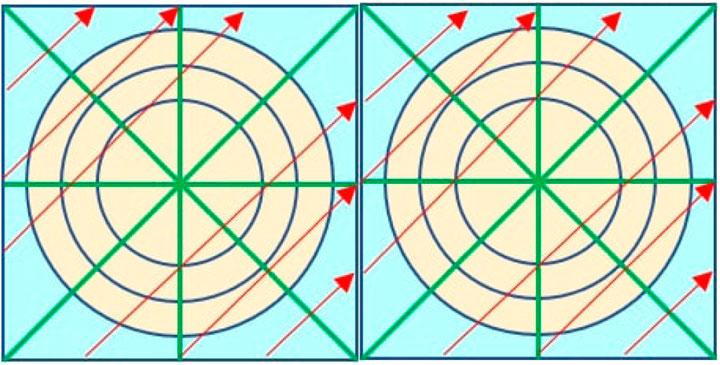
FIGURE 1. MOC discretization and rays.

Therefore, the outgoing flux of one segment is the incident flux of the adjacent next segment along the neutron flying direction. The incident flux $({\phi }_p^{in}(\mathrm{\Omega }))$, outgoing flux $({\phi }_p^{\mathit{out}}(\mathrm{\Omega }))$, and the track-average flux $({\bar{\phi }}_p(\mathrm{\Omega }))$ over each segment of the ray are computed as:

${\phi }_p^{\mathit{out}}\left(\mathrm{\Omega }\right)={\phi }_p^{in}\left(\mathrm{\Omega }\right)+\frac{{\phi }_p^d\left(\mathrm{\Omega }\right)}{x}x(8)$

$\frac{{\phi }_p^d\left(\mathrm{\Omega }\right)}{x}=\left[\frac{Q\left(\mathrm{\Omega }\right)}{{\mathrm{\Sigma }}_t}-{\phi }_p^{in}\left(\mathrm{\Omega }\right)\right]\frac{1-e^{-x}}{x},x={\mathrm{\Sigma }}_t\frac{l_p}{\sin \theta }(9)$

${\bar{\phi }}_p\left(\mathrm{\Omega }\right)=\frac{Q\left(\mathrm{\Omega }\right)}{{\mathrm{\Sigma }}_t}-\frac{{\phi }_p^d\left(\mathrm{\Omega }\right)}{x}(10)$

The reason why ${\varphi }_p^d(\mathrm{\Omega })/x$ is used here instead of ${\varphi }_p^d(\mathrm{\Omega })$ is to avoid the potential loss of significance for very small x in Eqs 8–10. Given that there are abundant tracks with different azimuthal angles within each computational region, the overall average flux $(\bar{\phi }(\mathrm{\Omega }))$ in a flat-source region (FSR) can be determined by the track-average fluxes and the track lengths of all enclosed characteristic rays as

$\bar{\phi }\left(\mathrm{\Omega }\right)=\frac{{\sum }_p{\bar{\phi }}_p\left(\mathrm{\Omega }\right)l_p\left(\mathrm{\Omega }\right)}{{\sum }_p{l}_p\left(\mathrm{\Omega }\right)}=\sum _p{\bar{\phi }}_p\left(\mathrm{\Omega }\right)l_p\left(\mathrm{\Omega }\right)\frac{C_{\mathrm{\Omega }}{\mathrm{\Delta }}_{\mathrm{\Omega }}}{A}(11)$

where C_Ω = A/(Δ_Ω ∑_pl_p(Ω)), and Δ_Ω is the ray-spacing distance for the direction Ω.

2.2 1D Transient NEM

Integrating the 1D equation obtained from Eq. 6 over a 4π solid angle and combining with Fick’s law gives the transverse integrated 1D diffusion equation, which can be further simplified as the 1D transient NEM equation when the cross-sections are considered uniform in a plane:

$-D_g^n\frac{{\partial }^2}{\partial z^2}{\varphi }_g^n\left(z\right)+{\mathrm{\Sigma }}_{rg}^n\left(z\right){\varphi }_g^n\left(z\right)-\sum _{g^{\prime }\ne g}{\mathrm{\Sigma }}_{g^{\prime }g}^n{\varphi }_{g^{\prime }}^n\left(z\right)-{\chi }_g{S}_F^n\left(z\right)=S_{\mathit{trg}}^{n-1}\left(z\right)+S_{\mathit{ntg}}^n\left(z\right)-L_{0,g}^n\left(z\right)(12)$

The quadratic leakage in the 1D problem depends on the average leakages of the investigating node and its left and right neighbors. For this reason, the transverse leakage and the transient source here are approximated by the conventional second-order Legendre polynomial:

$S_g\left(\xi \right)=\sum _{i=0}^2{s}_{g,i}{P}_i\left(\xi \right)(13)$

where P_i(ξ) are the standard Legendre polynomials, and the quadratic expansion coefficients (s_g,i) are determined by the node-average transverse leakages and thickness of the node of interest $({\bar{s}}_g^c,h_c)$ and its left and right neighbors $({\bar{s}}_g^l,{\bar{s}}_g^r,h_l,h_r)$. Similarly, the flux is estimated by a fourth-order Legendre polynomial:

${\varphi }_g\left(\xi \right)=\sum _{i=0}^4{a}_{g,i}{P}_i\left(\xi \right)(14)$

For a two-node problem, 10 constraints are required to solve the coefficients (a_g,i) for each energy group, including the two nodal average fluxes (2), the flux continuity (1) and current continuity (1) at the interface of two adjacent nodes, and the three weighted residual equations for each node (6). More details could be found in Hao et al. (2018).

2.3 CMFD acceleration

The transport equation for large nuclear reactors is generally difficult to solve; however, with the aid of the CMFD technique, the neutron diffusion equation can converge to the iterative solutions quite efficiently. Therefore, the multi-level CMFD acceleration method is used to find the transport currents in both steady-state and transient modules. In the multi-level CMFD, once the multigroup (MG) node average flux and the surface current are ready, the one-group (1G) parameters can be updated accordingly. This new 1G CMFD linear system renders the next generation of 1G flux distribution, which will be used to update the MG flux parameters to speed the eigenvalue convergence. Meanwhile, given that the CMFD equations are typical large sparse asymmetric linear systems Ax = b, where A is the sparse matrix for the neutron properties and interactions with each other and surrounding materials, and b is the source term, the preconditioned generalized minimal residual method (GMRES) is employed because it can take advantage of the sparsity of the matrix and is easy to implement (Saad, 2003). In addition, Givens rotation is considered in the GMRES solver because it can preserve better orthogonality and is more efficient than other processes for the QR factorization of the Hessenberg matrix, which has only one non-zero element below its diagonal. More details can be found in Tao and Xu (2020) and Xu and Downar (2012).

2.4 Code structure

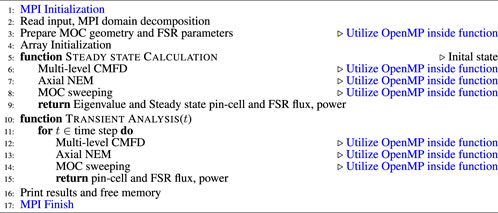
PANDAS-MOC is being developed using the C language at Purdue University. The code is capable of performing steady-state standalone analysis and the combination of steady-state and transient analysis based on the users’ requirements; its simplified workflow is illustrated in Figure 2A. In this work, we will focus on the performance of the steady-state module; its simplified flowchart is shown in Figure 2B. The flowchart for the transient calculation is omitted for brevity and can be found in Tao and Xu (2022b).

FIGURE 2

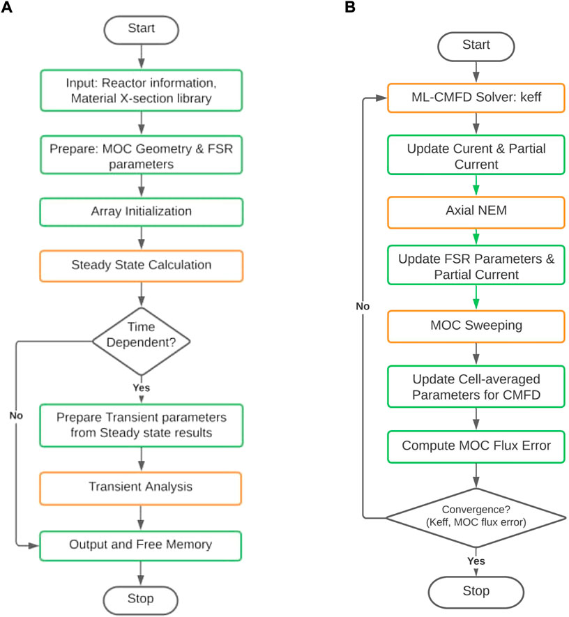
FIGURE 2. Flowchart of the PANDAS-MOC and the steady-state module. (A) PANDAS-MOC code structure; (B) scheme of steady-state analysis.

3 Parallelism

Parallel computing allows different portions of the computation to be operated concurrently by multiple processors to solve a single problem. Compared to conventional serial computing, it is more efficient with regard to the run time and memory because it often scales the problem size to execute the code on more processors, which makes it a good choice for solving a problem that involves large memory demands and intensive computations.

The current primary parallel standards are the message-passing interface (MPI) and the open multi-processing (OpenMP). The MPI is used for distributed memory programming, which means that every parallel processor is working in its own memory space, isolated from the others. OpenMP is applied for shared memory programming, which means that every thread has access to all the shared data. In addition, OpenMP is executed based on threads and performs parallel by explicitly inserting “#pragma omp” pragmas into the source code. It is intuitive to think that the communication between OpenMP threads is faster than the communication between the MPI processors, as it needs no internode synchronization. In addition, given that modern parallel machines have mixed distributed and shared memory, the hybrid MPI/OpenMP parallelization should also be considered to take advantage of such memory architecture. Normally, the hybrid parallel model uses MPI to communicate between the nodes and OpenMP for parallelism on the node. Therefore, it can eliminate the domain decomposition and provide automatic memory coherency at the node level and has lower memory latency and data movement with the node (Quinn, 2003).

Generally, the first step of performing parallelism is breaking the large problem into multiple smaller discrete portions, which is called decomposition or partitioning, and then arranging the synchronization pointers, such as barriers, to assure the correctness of computations. If the workload among the processors is distributed in an unbalanced fashion, some processors might be idle, waiting for the processors with heavier loads, which consequently creates a bottleneck for improving the parallel performance. In other words, good load balance can help maximize the parallel performance, and it is directly determined by the partitioning algorithm.

The measurement of parallel performance is the speedup (S), which is defined as the ratio of the sequential run time (T_s) (approximated using the run time with one processor (T₁)) and the parallel run time while using p processors (T_p). Also, efficiency (ϵ) is a metric of the utilization of the resources of the parallel system, the value of which is typically between 0 and 1.

$S_p=\frac{T_s}{T_p}\approx \frac{T_1}{T_p},{ϵ}_p=\frac{S_p}{p}(15)$

According to Amdahl’s law (Quinn, 2003), the maximum speedup S_p that can be achieved when using p processors depends on the sequential fraction of the problem (f_s).

$S_p=\frac{1}{f_s+\frac{1-f_s}{p}}\to \underset{p\to \infty }{\lim }{S}_p=\frac{1}{f_s}(16)$

For example, if 10% of the work in a problem remains serial, then the maximum speedup is limited to 10× even if more computing resources are employed. Therefore, real applications generally have sublinear speedup (S_p < p), due to the parallel overhead, such as task start-up time, I/O, load balance, data communications and synchronizations, and redundant computations.

This study is conducted in the “Current” cluster at Purdue University. Its mode is an Intel(R) Xeon(R) Gold 6152 CPU @ 2.10 GHz. It has two nodes and 22 CPUs for each node.

4 Test problem

The parallel performance of designed codes in this work are determined by a steady-state problem, in which all control rods are kept out of the C5G7 3D core from the OECD/NEA deterministic time-dependent neutron transport benchmark, which is proposed to verify the ability and performance of the transient codes without neutron cross-sections spatial homogenization above the fuel pin level (Hou et al., 2017) (Boyarinov et al., 2016). It is a miniature light water reactor with eight uranium oxide (UO₂) assemblies, eight mixed oxide (MOX) assemblies, and a surrounding water moderator/reflector. In addition, the C5G7 3D model is a quarter-core, and fuel assemblies are arranged in the top-left corner. For the sake of symmetry, the reflected condition is used for the north and west boundaries, and the vacuum condition is considered for the remaining six surfaces. Figure 3A is the planar and axial configuration of the C5G7 core. The size of the 3D core is 64.26 cm × 64.26 cm × 171.36 cm, and the axial thickness is equally divided into 32 layers.

FIGURE 3

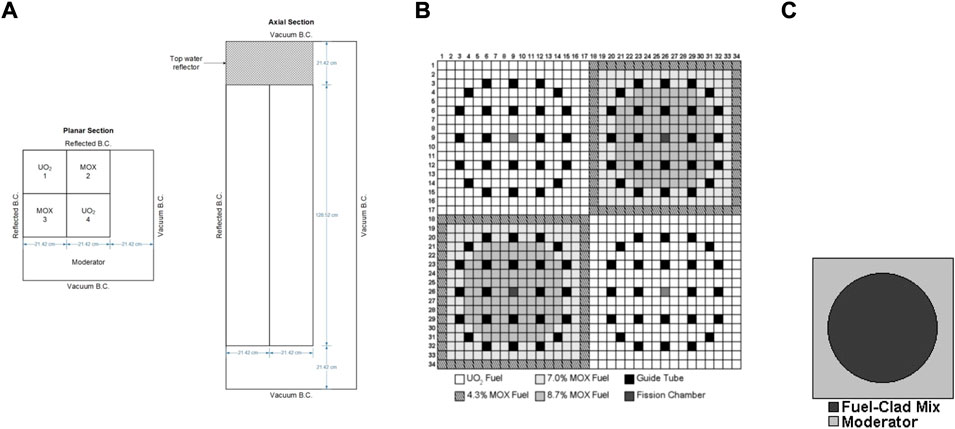
FIGURE 3. Geometry and composition of the C5G7-TD benchmark. (A) Planar and axial view of 1/4 core map; (B) fuel pin compositions and number scheme; and (C) pin cell.

The UO₂ assemblies and MOX assemblies have the same geometry configurations. The assembly size is 21.42 cm × 21.42 cm. There are 289 pin cells in each assembly arranged as a 17 × 17 square (Figure 3B), including 264 fuel pins, 24 guide tubes, and one instrument tube for a fission chamber in the center of the assembly. The UO₂ assemblies contain only UO₂ fuel, while the MOX assemblies includes MOX fuels with three levels of enrichment: 4.3%, 7.0%, and 8.7%. In addition, each pin is simplified as two zones in this benchmark. Zone 1 is the homogenized fuel pin from the fuel, gap, cladding materials, and zone 2 is the outside moderator (Figure 3C). The pin (zone 1) radius is 0.54 cm, and the pin pitch is 1.26 cm.

As for the geometry discretization, the calculations are performed with a Tabuchi–Yamamoto quadrature set with 64 azimuthal angles and three polar angles, and the spacing of MOC rays is 0.03 cm. The spatial discretization uses eight azimuthal flat source regions for each pin cell and three radial rings in the fuel cells (Figure 1). The moderator cells are divided into 1 by 1 coarse mesh or 6 by 6 finer mesh according to their locations in the core. In addition, the convergence criterion for the GMRES in the ML-CMFD solver is set as 10^–10, the convergence criterion for the eigenvalue is 10^–6 and for the flux is 10^–5. No preconditioners are called to show the improvement brought by the parallelism.

5 Parallel models and performance

5.1 Pure MPI parallel model

5.1.1 Design

In this model, the entire work is partitioned by multiple MPI processors, so that each processor undertakes a part of the calculation simultaneously. The fundamental concept is to divide the whole core problem (original domain) into various smaller tasks (subdomains), and each task has a manageable size for an individual processor. Figure 4 is an example of the domain decomposition implemented in this parallelization. A problem with a large domain (100cm × 75 cm × 100 cm) can be divided into 4 × 3 × 4 subdomains when executing 48 processes. Hence, the size of each subdomain is 25cm × 25 cm × 25 cm, and they are assigned to MPI processors with one-to-one correspondence. Subdomains can be further divided into multiple cells by the finite difference methods with respect to the solution accuracy, and each cell has six adjacent neighbors in the west, east, north, south, top and bottom sides.

FIGURE 4

FIGURE 4. MPI domain decomposition example. (A) Whole problem domain (B) MPI domain decomposition (C) One sub-domain (D) Cell and neighbors.

Following this idea, the spatial decomposition in PANDAS-MOC is handled by the MPI, and it has two levels: manual decomposition and cell-based decomposition. Users may manually enter a preferred number of subdomains in x, y, and z directions, which is also the number of MPI processors applied in each direction. The code will then partition the pin-cells automatically according to the entered number to enforce that the number of pin-cells assigned to each MPI processor are as balanced as possible.

Based on the domain decomposition, the PMPI code is developed with a similar structure to the serial code, except that multiple synchronization points are included in the parallel algorithms, such as MPI barriers, and data communication or reduction. First, the data exchange happens at the cells locating near the interface of the subdomains. In the neutron transport problem, various parameters are globally shared among all MPI distributed memories, such as the cross-sections, diffusion coefficients, non-discontinuity factors, partial current, and flux. It is necessary to communicate with other processors about those terms across the subdomains to perform the calculation correctly. Therefore, additional ghost memories are required to store the data received from the neighboring subdomains, and those data exchanges between processors are performed by MPI routines such as MPI_sendrecv(), MPI_Send(), and MPI_Recv(). Second, the reduction operation is a procedure generating the overall results using the partial results from all involved subdomains by the MPI routines like MPI_Allreduce(). Because those collective manipulations can only be performed until all processors has reached the same position to read, write, and/or update the latest information from/to all the involved processors, they will introduce communication overhead to the parallel performance.

The algorithm of PMPI model is described in Algorithm 1. For brevity, here only the key steps in PANDAS-MOC are listed. In the CMFD solver, each thread has its own local matrix A and local vectors b because of the domain decomposition. Then, to determine the global flux, data communications and reductions across all MPI processors are required. Particularly, the CMFD result of a cell is affected by the coefficients of its six neighbors, which could be located in different subdomains. Then, MPI_Send() and MPI_Recv() are employed to exchange the necessary data to perform the matrix–matrix or matrix–vector productions. In addition, MPI_Allreduce() is essential to determine the change of variables between two consecutive iterations, such as infinity-norm of flux change or source change. While in the MOC sweeping, the message passing is required for the angular flux of each characteristic ray starting at the subdomain boundary, and reduction is only needed to update the average flux for each FSR (Eq. 11).

Algorithm 1

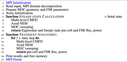
Algorithm 1. PMPI algorithm.

5.1.2 Performance

Table 1 describes the total MPI processors applied for the 3D benchmark problem and their distribution in the x, y and z directions. Tests were divided into two categories: partition on axial direction standalone and partition on all directions. The axial layers were assigned to MPI processors as equally as possible for all tests to achieve better load balance, as were the pin cells in the x-y plane. All tests are repeated five times to eliminate systematic error, and the average run time is employed for performance analysis.

TABLE 1

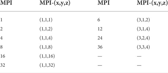
TABLE 1. MPI distribution for 3D problems.

All estimated k_eff are equal to 1.165,119 with negligible error $(\sim 10^{-8})$, which is the same as the eigenvalue obtained in the TD4/5 results in Tao and Xu (2022b). The outer iterations of the multi-level CMFD solver within the steady-state calculation are presented in Figure 5A. This figure reveals that tests having MPI domain decomposition only on the axial direction can provide a consistent converged eigenvalue with a consistent iteration number. In contrast, tests partitioned on all directions converged to a similar eigenvalue with 5–10 more iterations because of the round-off error accumulated from reduction operations with different arithmetic orders.

FIGURE 5

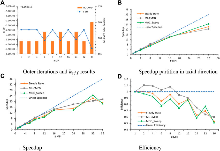
FIGURE 5. PMPI performance for the 3D problem. (A) Outer iterations and k_eff results (B) Speedup partition in axial direction (C) Speedup (D) Efficiency.

Table 2 has tabulated the run time for the entire steady-state calculation and the essential functions (ML-CMFD, NEM, and MOC sweep) when using one MPI processor. Note that three essential functions altogether have cost 85% of the run time of the steady-state calculation. The remaining 15% of the time is consumed by updating the MOC parameters with the CMFD results and vice versa, including evaluating cell-averaged flux and homogeneous cross-section for each cell from the MOS swept FSR flux, estimating the current coupling coefficient with partial currents on each cell surface, updating the scale flux of each FSR and angular flux on the system boundary from CMFD solutions, and preparing the fission and scattering source for each FSR with FSR scalar flux. Furthermore, compared to the time consumed by the ML-CMFD solver and the MOC sweep solver, the NEM time is $<1\%$ of the total run time. Here, it can also be observed that the CMFD solver takes a relatively large portion of the overall computational effort. The reason for such behavior is that the MG and 1G CMFD linear systems constructed during each iteration are nearly singular or ill-conditioned and require many iterations to solve. Consequently, the following analysis will focus on the ML-CMFD and MOC sweep solvers, even though the parallel strategies investigated in the work can effectively accelerate other calculations as well. Treating run time with one MPI processor (T₁) as the sequential time (T_s), the parallel speedup and efficiency are evaluated and plotted in Figure 5.

TABLE 2

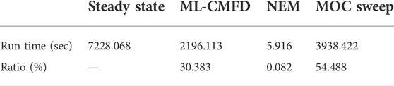
TABLE 2. Measured run time of key functions of steady-state calculation using one MPI processor.

Figure 5B depicts the speedup obtained from the tests with solely axial MPI domain decomposition, in which the executed numbers of MPI processors were 2^k (k = 1, 2, … , 5). Because MOC sweeping has consumed around 55% of the overall steady-state run time, the steady-state speedup approaches the MOC sweep speedup. In this scenario, the measured speedup was close to the linear speedup at first and then deviated when more MPI processors were involved. The parallelization overhead is caused by the unbalanced workload. Considering that the top four and bottom four layers of the benchmark core are composed of moderators while the central 28 layers are the fuel region, the corresponding computational tasks will be very different due to the different pin-cell compositions and discretization styles. The workload distribution becomes more biased when adding more MPI processors, although the number of layers in each subdomain remains the same.

Figures 5C,D include the speedup and efficiency of all measured tests, showing that contributing more processors will increase the speedup. However, having domain decomposition in the x and y directions will hurt the parallel efficiency to some extent; the more synchronization points, the greater the synchronization execution latency overhead. Although all subdomains are allowed to solve their local problems concurrently, interior subdomains will not have the boundary conditions ready until they have been exchanged through all other subdomains across the interior interfaces and the problem boundaries. Among three measurements, this is most evident in the MOC sweep. To perform the MOC sweeping along each long characteristic track, the outgoing angular flux at the previous subdomain is considered as the incident value for the next subdomain. As a result, the overhead in communicating the information across the subdomain interfaces is unavoidable.

5.2 Segment OpenMP threading hybrid model

5.2.1 Design

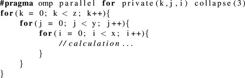
The previous PMPI model was built only based on the distributed memory model. The hybrid MPI/OpenMP programming is considered to develop another parallel model of PANDAS-MOC and take advantage of the hybrid distributed and shared memory architecture on modern computing machines. Starting from the framework of MPI domain decomposition and the finite difference methods, the OpenMP pragmas are added ahead of the spatial for-loops to partition the calculation. As depicted in Figure 6, when enacting four OpenMP threads, the cells within an MPI subdomain are partitioned into four groups. Specifically, the OpenMP parallel regions are mostly the for-loops, and their work-sharing constructs are specified by the “#pragma omp parallel for” statement with a series of clauses, such as private, reduction, or collapse, which depends on the purpose of the associated calculations. For example:

FIGURE 6

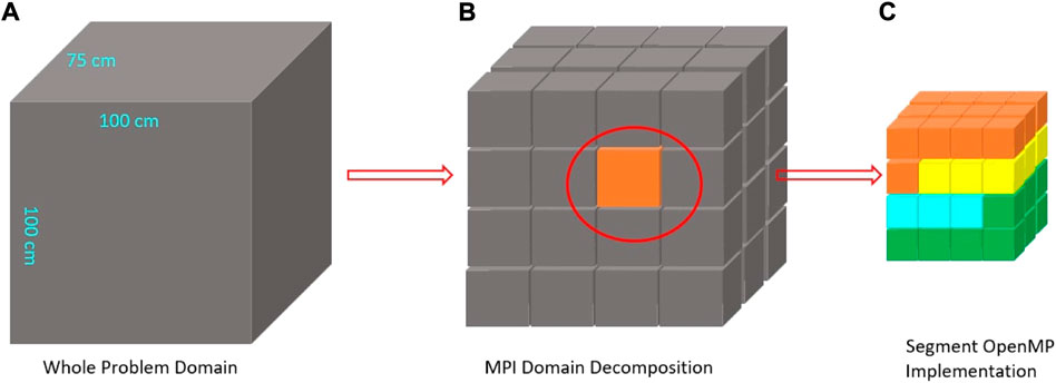
FIGURE 6. Segment OpenMP threading example. (A) Whole problem domain (B) MPI domain decomposition (C) Segment OpenMP implementation.

Because the OpenMP parallelism does not involve in the domain decomposition but the functional decomposition and only manages a piece of calculation, this code is named the Segment OpenMP threading hybrid model (SGP), and its algorithm is described in Algorithm 2. Given that inserting the OpenMP directives does not change the code structure and iterative scheme, SGP has an algorithm very similar to the algorithm of the PMPI code (Algorithm 1). However, considering that the OpenMP parallelism needs to be created and destroyed each time the “#pragma omp parallel” is called, the SGP model has extra OpenMP construction overhead in addition to the drawbacks of the PMPI model, which will discount the parallel performance to some extent.

Similar to the PMPI model, data synchronization is still essential to the correctness of the SGP code. In hybrid MPI/OpenMP parallelization, reduction is conventionally performed by two steps. The first step is the OpenMP reduction, in which the partial result in each individual OpenMP thread is collected by the omp reduction clause to generate the local result for the corresponding MPI processor. The second step is using the MPI routines like MPI_Allreduce() or MPI_Reduce() to gather and compute the global result as in the PMPI model. Meanwhile, OpenMP offers several options to synchronize the threads, such as critical, atomic, and barrier. The SGP model relies on the “atomic” and implicit/explicit “barrier” to avoid a potential race condition and guarantee synchronization. Furthermore, the synchronization points pertaining to the MPI processors are defined similarly to those in the PMPI model.

Algorithm 2

Algorithm 2. SGP algorithm.

5.2.2 Performance

The parallel performance is examined by the 3D problem with the identical geometry discretization, numerical conditions, and parallel setup in Section 5.1. The tested numbers of the MPI processor and OpenMP threads are tabulated in Table 3. All runs were repeated five times to avoid systematic measurement error, and the average run time was considered for the parallel performance analysis. The speedup for the overall steady state, ML-CMFD solver, and MOC sweep module is computed based on the run time cost by the PMPI model using one MPI processor (Table 2). All tests could be separated into three categories, although some tests may exist in multiple categories at the same time:

TABLE 3

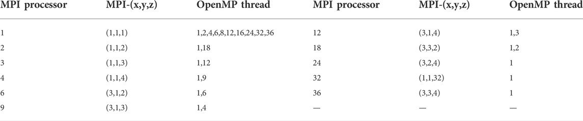
TABLE 3. Number of MPI processors and OpenMP threads for 3D problems.

Category 1: m ≥ 1 MPI processors and p = 1 OpenMP thread.

Category 2: m = 1 MPI processor and p ≥ 1 OpenMP threads.

Category 3: m MPI processors and p threads, and m × p = 36.

The important overheads induced by the algorithm per se are described in Table 4. In addition, Figures 7A,B compare the steady-state speedup and efficiency of the PMPI model (green line), Category 1 of the SGP model (blue line), and Category 2 of the SGP model (orange line), and it demonstrates that the segment-threading implementation is not as efficient as the pure MPI implementation. To further explore the factors that jeopardize the speedup in each essential module, the speedup of the ML-CMFD solver and MOC sweep are plotted in Figure 7.

TABLE 4

TABLE 4. Key overheads in different tests (○: does not exist, ⊗: exists).

FIGURE 7

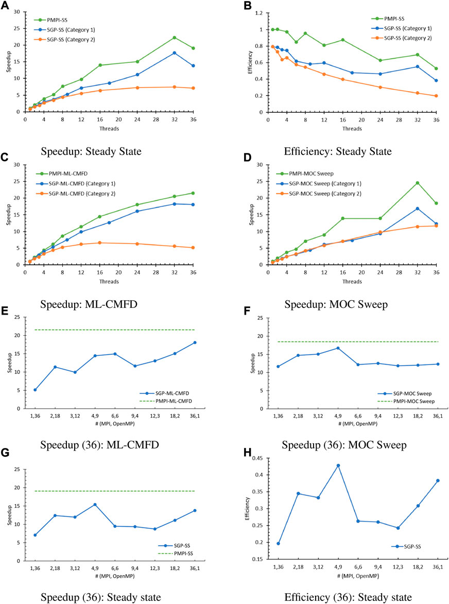
FIGURE 7. SGP parallel performance (36: category 3). (A) Speedup: Steady State, (B) Efficiency: Steady State, (C) Speedup: ML-CMFD, (D) Speedup: MOC Sweep, (E) Speedup (36): ML-CMFD, (F) Speedup (36): MOC Sweep, (G) Speedup (36): Steady state, (H) Efficiency (36): Steady state.

Concerning the ML-CMFD solver (Figure 7C), tests in Category 1 had one OpenMP thread executed, hence the single difference compared to the PMPI model is that the SGP model repetitively creates and destroys the OpenMP region when the omp parallel directive is explicitly stated. Thus, the gap between the green and blue lines has confirmed the overhead brought by such thread initialization and finalization. Furthermore, when executing a single MPI processor and multiple OpenMP threads, the tests in Category 2 also suffered from the initialization issue, which, nevertheless, was not the principal reason for the unsatisfactory performance. Given that the major work in the ML-CMFD solver is the matrix–matrix, matrix–vector, and vector–vector productions, the MPI/OpenMP reduction procedure needs to be performed frequently. Here, the reduction procedure and waiting time brought by implicit and explicit barriers cost more time and slowed the calculation. This effect becomes more severe when more OpenMP threads are involved due to the nature of OpenMP parallelization on for-loops.

On the other hand, in the MOC sweep (Figure 7D), Category 1 and Category 2 presented similar speedups, which are smaller than the PMPI, due to the limited starting and ending times of the OpenMP parallelization. For example, for SGP tests using threads (36,1), the steady state converged after 28 outer iterations, which indicates that the code has swept the MOC rays 28 times, and the “#pragma omp parallel for” directive has been enacted for 896 (= 28 × 32) times in the MOC sweep part. Therefore, the time cost of these directives is negligible in contrast to the entire time spent by the MOC sweep, which is around 320 s. The factor that diminished the speedup of MOC solver is the omp atomic clause, which ensures that a specific storage location is accessed atomically, rather than exposing it to the multiple simultaneous reading and writing threads that may result in indeterminate values. To verify this speculation, removing the “#pragma omp atomic” statement from the SGP code was tested. Using (36, 1), when running without the omp atomic clause, the measured run time for the MOC solver is 188.123 s, while the MOC solver with the omp atomic clause consumed 319.759 s. This test pinpointed that the atomic construct itself used more than 40% of the MOC run time.

Tests having the total number of threads as 36 (Category 3) were conducted to study the hybrid parallel performance. The collected speedup of the ML-CMFD solver and the MOC sweep are plotted in Figures 7E,F, respectively, where the dotted green lines are the PMPI performance with 36 MPI processors. Even though all speedup results are not comparable to the PMPI speedup using 36 MPI processors, the ML-CMFD and MOC sweep presented different tendencies. Among all tests, the ML-CMFD solver has the best speedup at (36,1). MPI dominated the performance improvement in this part because of the limitation of the OpenMP parallel overhead from repetitious construct and destruct and synchronization points, which was demonstrated in the previous discussion. In contrast, the speedup of MOC sweep at all groups of MPI processors and OpenMP threads is larger than or at least close to the speedup at (36,1), and (4,9) has achieved the largest speedup because of its better load balance. The speedup and efficiency for the entire steady-state calculation are shown in Figures 7G,H. Similar to the MOC sweep performance, tests with (4,9) achieved the best speedup for the overall steady-state calculation. The corresponding optimal parallel efficiency is around 0.428 and is smaller than 0.529, which is the PMPI efficiency while running 36 MPI processors.

5.3 Whole-code OpenMP threading hybrid model

5.3.1 Design

Considering that the repeated creation and destruction of the OpenMP regions could significantly lower the parallel performance of the OpenMP threading, especially in the CMFD part, this model deliberately treats the entire project as a unit and uses MPI and OpenMP to partition it simultaneously to avoid such impacts. Therefore, this model is named the whole-code OpenMP threading hybrid model (WCP). Figure 8 is an example of the domain decomposition in WCP. The original problem domain is partitioned by four MPI processors, and each processor further spawns 27 OpenMP threads to split the work within each subdomain. Each color in the right-hand plot identifies an MPI subdomain, and each cubic represents the OpenMP decomposition. Here, the code creates 108 (= 4*27) subdomains, but the required amount of ghost memories and inter-processor communications are similar to the case using four MPI processors and one OpenMP thread, given that increasing the number of OpenMP threads does not ask for more memory, as does the number of MOC sweeps. The consumed memory in this model is expected to be much less than the PMPI model when the same number of total threads is executed, which will be discussed in Section 5.4. In this way, OpenMP parallelism is established immediately after the MPI initialization (MPI_Init, MPI_Comm_size, MPI_Comm_rank) and destroyed right before the MPI finish (MPI_Finalize). This design will reduce the OpenMP construction overhead to a negligible level because there is only one creation and destruction of OpenMP parallelization through the entire code, and it is capable of omitting many unnecessary barriers to shrink the waiting time among threads. Other than that, the treatment of reduction and synchronization is similar to that in SGP. By introducing the OpenMP to this model, thread-private variables and global-shared variables are further specified while launching the OpenMP threads to prevent potential race condition issues. Additionally, the data synchronization is completed by OpenMP and MPI cooperatively. For example, the reduction process is still performed by the omp reduction clause and the MPI_Allreduce routine. One thing worth mentioning is that the MPI routines inside the OpenMP parallelization region should be performed by a single OpenMP thread, such as MPI_Allreduce() or MPI_Sendrecv(). Other than that, the code flow and iteration scheme are maintained similarly to the previous models, and the algorithm of WCP is listed in Algorithm 3.

Algorithm 3

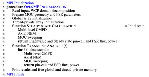
Algorithm 3. WCP algorithm.

FIGURE 8

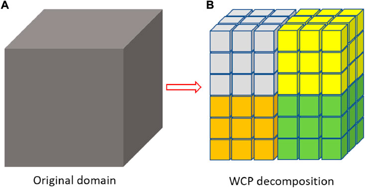
FIGURE 8. Whole-code OpenMP threading example. (A) Original domain (B) WCP decomposition.

5.3.2 Performance

The performance of the WCP model was assessed by repeating the numerical experiments for the SGP model and using the number of threads listed in Table 3. All runs were tested five times to avoid systematic measurement error, and the average run time was considered for the parallel performance analysis. The speedup of steady-state calculation, ML-CMFD solver, and MOC sweep are evaluated based on run time in Table 2 accordingly.

First, the speedup of the steady state while running with one OpenMP thread (Category 1) or one MPI processor (Category 2) is analyzed and illustrated in Figure 9A, along with the corresponding tendencies obtained in the previous PMPI and SGP models. The estimated speedup is still less than PMPI in all tested cases. On the other hand, the contrast between the Category 2 tests of the SGP model and the WCP model hints that WCP can effectively improve the performance when investing more OpenMP threads, in that the OpenMP environment and parallel chucks are constructed only once, and the number of implicit barriers has been greatly reduced in the WCP model.

FIGURE 9

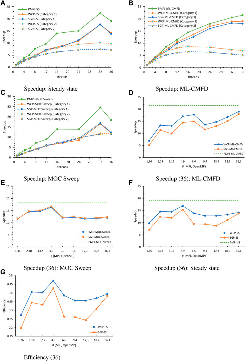
FIGURE 9. WCP parallel performance (36: category 3). (A) Speedup: Steady state, (B) Speedup: ML-CMFD, (C) Speedup: MOC sweep, (D) Speedup (36): ML-CMFD, (E) Speedup (36): MOC sweep, (F) Speedup (36): Steady state, (G) Efficiency (36).

To investigate the performance more closely, the speedup of the ML-CMFD solver and MOC sweep are depicted in Figures 9B,C. In the ML-CMFD plot, the WCP successfully improved the speedup for tests in both Category 1 and Category 2 due to less time consumed by the creation and destruction of OpenMP parallel regions and the implicit barriers. In contrast, the SGP and WCP offered similar performance for the MOC sweep part because of the trivial times of enacting the OpenMP blocks in the SGP model. Because the omp atomic directives are still kept for data synchronization in this function of the WCP model, it is still the principal issue in the parallelism of ray sweeping. Using (36, 1), the MOC calculation needs 326.646 s to finish while running the code with the atomic directives and needs 187.326 s while running without the atomic directives, which implies that the ratio of the atomic construction for the MOC calculation is still above 40%. For now, the code without atomic directives cannot be extended to cases using multiple OpenMP threads owing to the race condition. Nevertheless, it has shed light on how to further optimize the parallelization of MOC sweeping, which is thoroughly discussed in Tao and Xu (2022c).

Meanwhile, the speedup and efficiency of tests having 36 total threads are analyzed in Figures 9D–G. Similar to the previous tests, the WCP model can effectively improve the speedup in the ML-CMFD solver by decreasing the overhead caused by the initializing and finalizing of the OpenMP constructs and the synchronization points. Furthermore, (36,1) presented the best speedup again among all tests, which means that the overhead from the hybrid reduction is still a challenge in accelerating the multi-level CMFD calculation. In addition, the speedup of the MOC sweeping part in the WCP model and SGP model overlap each other, and the relative differences between the two models are smaller than 2% in all tests. Therefore, the parallel efficiency in this part is limited by the atomic structures that are crucial to the race-free conditions. The overall speedup and efficiency of the steady state are shown in Figures 9F,G. Except for (1,36), the evaluated speedup and efficiency are similar to or larger than that obtained by (36,1). The best result happens at (4,9) again, and the corresponding optimal parallel efficiency is 0.47, which is better than the SGP model (0.428) yet still less than the PMPI model (0.529). Moreover, the WCP speedup increased a substantial amount compared to the SGP model, especially for the tests having MPI domain decomposition in all x, y, and z directions. For example, the speedup at (6,6) improved by 46.30%, the speedup at (9,4) improved by 36%, and the speedup at (12,3) improved by 46.94%.

5.4 Memory comparison

Considering that there is only a single copy of the data in the shared-memory parallelization, regardless of the number of enacted threads, whereas each process has an individual and complete copy of all data with distributed-memory parallelization, the shared-memory parallelization requires much less memory than the distributed-memory parallelization. To demonstrate this advantage in the WCP model, the memory consumed by the PMPI and WCP models is measured by othe getrusage command, which returns the sum of resources used by all threads corresponding to the calling process. Specifically, the maximum resident set size usage is exploited as the actual resources used to complete the work. Because the usage values are returned for each processor, the total consumed memory is estimated as the sum of all active processors.

In addition, the consumed memory was measured at three points: 1) after MPI initialization; 2) after geometry setup and discretization and shared/thread-private arrays allocation; and 3) after the steady-state calculation. The collected memory usage data for these three parts in the PMPI model when executing 36 processors are 352968 kb, 15003744 kb, and 3545624 kb. Accordingly, the memory usage in the WCP was also measured by forcing the total number of threads to 36, and the corresponding ratio of the WCP model to the PMPI model is estimated and plotted in Figure 10. It is noticeable that the evaluated ratios at all tests and all measuring points are less than 1.0 (yellow dashed line), except for the test running with (36,1). In this test, the amounts of memory used by the geometry setup and memory allocation in the two models are similar to each other, but the WCP has cost 7.1% more memory in the MPI initialization and has saved 12.1% memory in the steady-state calculation compared to the PMPI model. Concerning the memory usage in the test using (4,9), which had the best parallel performance in the previous discussion, the assessed ratio of memory used in the MPI initialization, geometry setup and memory allocation, and steady-state calculation are 0.1096, 0.6167, and 0.5615, respectively, which has manifested the preeminence of the hybrid MPI/OpenMP parallelization from a memory perspective.

FIGURE 10

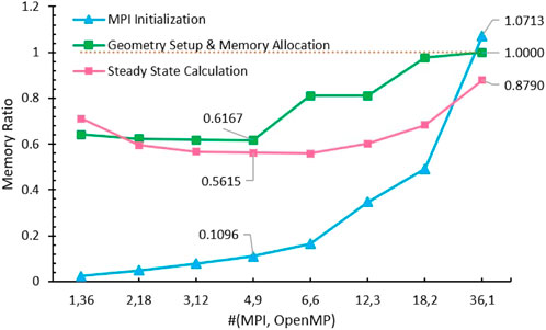
FIGURE 10. Ratio of memory used in WCP to PMPI (total number of threads = 36).

6 WCP optimizations

As discussed above, in spite of the memory advantages, the parallel performance achieved from the current version of the WCP model is better than the SGP model, which is the conventional fashion of hybrid MPI/OpenMP parallelism, yet not comparable to the PMPI model. In ongoing work, the optimizations on the hybrid reduction in ML-CMFD solver and parallelism of MOC sweeping are performed, and detailed discussions are presented in Tao and Xu (2022a) and Tao and Xu (2022c), respectively.

On the one hand, the reductions in the hybrid MPI/OpenMP codes are generally completed by the omp reduction clause and MPI reduction routines, which contain implicit barriers to slow the calculations. To eliminate such synchronization points, two new algorithms are proposed: Count-Update-Wait reduction and Flag-Save-Update reduction. Instead of waiting for all OpenMP threads to have their partial results ready, Count-Update-Wait reduction immediately gathers the data once a thread has finished its calculation and counts the number of partial results that have been collected. When all threads have rendered their partial results, the MPI_Allreduce routine is used in the zeroth OpenMP thread to compute the global result and reset the local variables and counts. Additionally, in the Flag-Save-Update reduction, two global arrays are defined to store the partial results and the status flag of each OpenMP thread, respectively, and the threads are configured as a tree structure to favor the reduction procedure. When all partial results are collected, the MPI_Allreduce routine is called to generate the global solution. Detailed information can be found in Tao and Xu (2022a). The first algorithm has fewer barriers than the conventional hybrid reduction yet introduces extra serializations, such as atomic or critical sections, to ensure that all partial results are collected from each enacted OpenMP thread. The second algorithm contains no barriers; the calculation flow is controlled by the status flags. In Tao and Xu (2022a), we demonstrated that the Flag-Save-Update reduction could provide a larger speedup than the Count-Update-Wait reduction and the conventional hybrid reduction algorithm, which nevertheless is still smaller than the MPI_Allreduce standalone in the PMPI model.

On the other hand, while using the OpenMP directives to partition the characteristic rays sweeping, the speedup of the MOC sweep is limited by the unbalanced workload among threads and the serialization overhead caused by the omp atomic clause for assuring the correctness of MOC angular flux and current update. Two schedules are designed to resolve these two obstacles: The Equal Segment (SEG) schedule and the No-Atomic schedule. The SEG resolves the unbalanced issue, in which the average number of segments is determined in the first step according to the total number of segments and number of executed threads, and then long tracks are partitioned based on this average number so that the segments (i.e., the actual computational workload) are distributed among the OpenMP threads as equally as possible. Based on SEG, the No-Atomic schedule further removes all omp atomic structures to improve computational efficiency by pre-defining the sweeping sequence of long-track batches across all threads to create a race-free job. The implementation details can be found in Tao and Xu (2022c). Repeating the same tests on each schedule confirms that the No-Atomic schedule is capable of achieving much better performance than the other schedules and even outperforms the PMPI sweeping with the identical total number of threads.

A comparison of the performance obtained from the PMPI (dashed blue line), the WCP using default methods as discussed in Section 5.3 (green line, labeled as (d)), and the optimized WCP (pink line, labeled as (o)) is illustrated in Figure 11. Although the ML-CMFD solver using the Flag-Save-Update reduction is still slower than the PMPI using MPI_Allreduce (Figure 11A), the advantage gained from the MOC sweep with No-Atomic schedule is large enough to compensate for such weakness (Figure 11B). Therefore, the optimized WCP code has managed to accomplish much better speedup than the original WCP code and is comparable to or even greater than the PMPI code, as explained in Figures 11C,D.

FIGURE 11

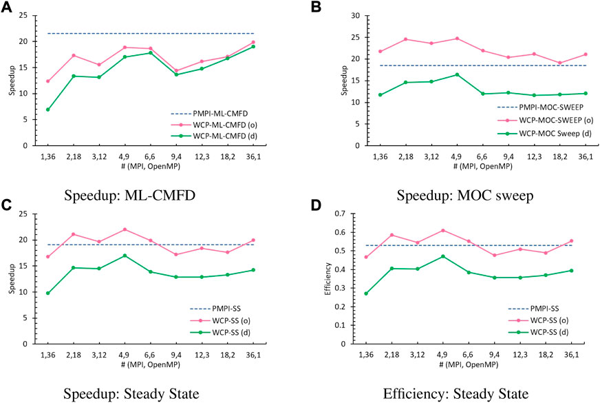
FIGURE 11. Performance comparison with 36 total threads (o: optimized algorithm, d: default method). (A) Speedup: ML-CMFD, (B) Speedup: MOC sweep, (C) Speedup: Steady state, (D) Efficiency: Steady state.

7 Conclusion

In this article, a PMPI model of the PANDAS-MOC is developed based on the distributed memory model, and the SGP and WCP models are designed based on the hybrid distributed and shared memory architecture. Their parallel performance is examined using the C5G7 3D core. For the PMPI model, tests with different numbers of processors all converged to the same eigenvalues with different iterations due to the round-off error accumulated from the arithmetic operations. In addition, it provided a sublinear speedup due to the load balance issue and communicating overhead between the MPI subdomains. Moreover, the measured speedups of the two hybrid models are smaller than the PMPI when executing the identical number of processors and/or threads, whereas WCP has better parallel performance than the SGP model. SGP was heavily affected by the repeated creation and destruction of the OpenMP parallelization, synchronization, and reduction in the ML-CMFD solver and omp atomic directives in the MOC sweeping. In the WCP model, the overhead caused by the repeated creation and destruction of the OpenMP regionsand by the omp barriers is resolved by intentionally dividing the entire work as a unit by the MPI and OpenMP simultaneously at the beginning of execution. Although the optimal parallel efficiency provided by the WCP model is 0.47, which is slightly smaller than the efficiency obtained in the PMPI model (0.529), we have determined the reasons that jeopardize the performance in both the ML-CMFD solver and the MOC sweep in this work: the hybrid reduction and omp atomic operations. In addition, the advantage of the hybrid MPI/OpenMP memory usage has been demonstrated for the WCP model. The estimated ratios of consumed memory in the WCP model for the arrays’ memory allocation and steady state were about 60% of those of the PMPI model, which makes this model promising from the memory perspective. This further inspires our future work on the development of advanced hybrid reduction algorithms and better MOC sweep schedules in the WCP model. Once these challenges are resolved, the optimized WCP model is expected to outperform the PMPI model.

Data availability statement

The original contributions presented in the study are included in the article/Supplementary material; further inquiries can be directed to the corresponding author.

Author contributions

All authors contributed to the conception and methodology of the study. ST performed the coding and data analysis under YX’s supervision and wrote the first draft of the manuscript. All authors contributed to the manuscript revision and read and approved the submitted version.

Conflict of interest

The authors declare that the research was conducted in the absence of any commercial or financial relationships that could be construed as a potential conflict of interest.

Publisher’s note

All claims expressed in this article are solely those of the authors and do not necessarily represent those of their affiliated organizations or those of the publisher, the editors and the reviewers. Any product that may be evaluated in this article, or claim that may be made by its manufacturer, is not guaranteed or endorsed by the publisher.

References

Boyarinov, V., Fomichenko, P., Hou, J., Ivanov, K., Aures, A., Zwermann, W., et al. (2016). Deterministic time-dependent neutron transport benchmark without spatial homogenization (c5g7-td). Paris, France: Nuclear Energy Agency Organisation for Economic Co-operation and Development NEA-OECD.

Google Scholar

Boyd, W., Shaner, S., Li, L., Forget, B., and Smith, K. (2014). The openmoc method of characteristics neutral particle transport code. Ann. Nucl. Energy 68, 43–52. doi:10.1016/j.anucene.2013.12.012

CrossRef Full Text | Google Scholar

Chen, J., Liu, Z., Zhao, C., He, Q., Zu, T., Cao, L., et al. (2018). A new high-fidelity neutronics code necp-x. Ann. Nucl. Energy 116, 417–428. doi:10.1016/j.anucene.2018.02.049

CrossRef Full Text | Google Scholar

Cho, Jin Young, Joo, Han Gyu, Kim, Ha Yong, and Chang, Moon-Hee (2003). Parallelization of a three-dimensional whole core transport code DeCART, In International Conference on Supercomputing in Nuclear Application, SNA03, Paris, France Sep 22, 2003. Available at https://www.osti.gov/etdeweb/servlets/purl/20542391.

Google Scholar

Choi, N., Kang, J., and Joo, H. G. (2018). “Preliminary performance assessment of gpu acceleration module in ntracer,” in Transactions of the Korean Nuclear Society Autumn Meeting, Yeosu, Korea, October 24-26 2018.

Google Scholar

Hao, C., Xu, Y., and Downar, J. T. (2018). Multi-level coarse mesh finite difference acceleration with local two-node nodal expansion method. Ann. Nucl. Energy 116, 105–113. doi:10.1016/j.anucene.2018.02.002

CrossRef Full Text | Google Scholar

Hou, J., Ivanov, K., Boyarinov, V., and Fomichenko, P. (2017). Oecd/nea benchmark for time-dependent neutron transport calculations without spatial homogenization. Nucl. Eng. Des. 317, 177–189. doi:10.1016/j.nucengdes.2017.02.008

CrossRef Full Text | Google Scholar

Jung, Y. S., Lee, C., and Smith, M. A. (2018). PROTEUS-MOC user manual. Tech. Rep. ANL/NSE-18/10, nuclear science and engineering division. Illinois: Argonne National Laboratory.

Google Scholar

Larsen, E., Collins, B., Kochunas, B., and Stimpson, S. (2019). MPACT theory manual (version 4.1). Ann Arbor, Michigan: University of Michigan, Oak Ridge National Laboratory. Tech. Rep. CASL-U-2019-1874-001.

Google Scholar

Quinn, M. (2003). Parallel programming in C with MPI and OpenMP. Boston: McGraw-Hill.

Google Scholar

Saad, Y. (2003). Iterative methods for sparse linear systems. 2nd Edition. Philadelphia, PA: Society for Industrial and Applied Mathematics.

Google Scholar

Tao, S., and Xu, Y. (2020). “Hybrid parallel computing for solving 3d multi-group neutron diffusion equation via multi-level cmfd acceleration,” in Transactions of the American Nuclear Society, June 8–11, 2020Virtual Conference 122, 421–424. doi:10.13182/T122-32578

CrossRef Full Text | Google Scholar

Tao, S., and Xu, Y. (2022a). Hybrid parallel reduction algorithms for the multi-level cmfd acceleration in the neutron transport code pandas-moc, Front. Nucl. Eng. 1, 1052332. doi:10.3389/fnuen.2022.1052332

CrossRef Full Text | Google Scholar

Tao, S., and Xu, Y. (2022b). Neutron transport analysis of c5g7-td benchmark with pandas-moc. Ann. Nucl. Energy 169, 108966. doi:10.1016/j.anucene.2022.108966

CrossRef Full Text | Google Scholar

Tao, S., and Xu, Y. (2022c). Parallel schedules for moc sweep in the neutron transport code pandas-moc, Front. Nucl. Eng. 1, 1002862. doi:10.3389/fnuen.2022.1002862

CrossRef Full Text | Google Scholar

Tao, S., and Xu, Y. (2021). “Reactivity insertion transient analysis for c5g7-td benchmark with pandas-moc,” in Transactions of the American Nuclear Society (2021 ANS Winter Meeting), Washington, DC, November 30–December 3, 2021, 938–941.125

Google Scholar

Xu, Y., and Downar, T. (2012). “Convergence analysis of a cmfd method based on generalized equivalence theory,” in PHYSOR 2012: Conference on Advances in Reactor Physics - Linking Research, Industry, and Education, Knoxville, United States, 15-20 Apr 2012.

Google Scholar