A new transfer entropy method for measuring directed connectivity from complex-valued fMRI data

Background: Inferring directional connectivity of brain regions from functional magnetic resonance imaging (fMRI) data has been shown to provide additional insights into predicting mental disorders such as schizophrenia. However, existing research has focused on the magnitude data from complex-valued fMRI data without considering the informative phase data, thus ignoring potentially important information.

Methods: We propose a new complex-valued transfer entropy (CTE) method to measure causal links among brain regions in complex-valued fMRI data. We use the transfer entropy to model a general non-linear magnitude–magnitude and phase–phase directed connectivity and utilize partial transfer entropy to measure the complementary phase and magnitude effects on magnitude–phase and phase–magnitude causality. We also define the significance of the causality based on a statistical test and the shuffling strategy of the two complex-valued signals.

Results: Simulated results verified higher accuracy of CTE than four causal analysis methods, including a simplified complex-valued approach and three real-valued approaches. Using experimental fMRI data from schizophrenia and controls, CTE yields results consistent with previous findings but with more significant group differences. The proposed method detects new directed connectivity related to the right frontal parietal regions and achieves 10.2–20.9% higher SVM classification accuracy when inferring directed connectivity using anatomical automatic labeling (AAL) regions as features.

Conclusion: The proposed CTE provides a new general method for fully detecting highly predictive directed connectivity from complex-valued fMRI data, with magnitude-only fMRI data as a specific case.

1 Introduction

To date, a huge number of studies have investigated directed functional connectivity (FC) or functional network connectivity (FNC) using fMRI data (Demirci et al., 2009; Stevens et al., 2009; Lizier et al., 2011; Ursino et al., 2020; Crimi et al., 2021). Directed FC/FNC refers to the statistical causality between different time series from brain regions of interest (ROIs) or time courses of brain networks extracted by data-driven methods from fMRI data (Stevens et al., 2009; Ursino et al., 2020; Mahmood et al., 2022). The directed FC/FNC results have been widely used as putative biomarkers to identify/predict brain function changes linked to mental disorders such as schizophrenia (Fogelson et al., 2014; Bastos-Leite et al., 2015; Dietz et al., 2020).

Directed FC/FNC analyses can be generally classified into model-based and model-free methods. Typical model-based methods include dynamic causal modeling (DCM) (Friston et al., 2019), structural equation modeling (Bielczyk et al., 2019), and dynamic Bayesian network (Wu et al., 2014). Regarding model-free methods, the Granger causal test is frequently used to determine whether there is a linear causal relationship between ROIs and brain networks (Demirci et al., 2009; Crimi et al., 2021). Demirci et al. (2009) exploited the Granger causal test to calculate directed FNC of fMRI data and found abnormal connections from frontal areas to visual areas for patients with schizophrenia. Crimi et al. (2021) used Granger connections to classify patients with autism spectrum disorder and healthy controls.

Real-valued transfer entropy is utilized to identify the underlying non-linearly directed information between ROIs or between brain networks (Lizier et al., 2011; Ursino et al., 2020; Liu et al., 2022). Ursino et al. (2020) verified that transfer entropy is a promising method to estimate the causality of connections between regions with long time delays. Lizier et al. (2011) presented a transfer entropy method to detect causality between brain regions in cognitive tasks and showed task difficulty being related to causal strength for the motor cortex. Following this, Liu et al. (2022) proposed a scored function based on transfer entropy and conditional entropy to quantify directed FC, which accurately inferred directed connectivity networks of time series. The most commonly used method for estimating real-valued transfer entropy is the histogram-based transfer entropy (HTE), which estimates the joint probability density function via a histogram-based function. Other transfer entropy algorithms were proposed to improve the accuracy of causal inference or noise robustness, including symbolic transfer entropy (STE) (Li and Zhang, 2022), effective transfer entropy (Behrendt et al., 2019; Caserini and Pagnottoni, 2022), Renyi transfer entropy (Jizba et al., 2022; Zhang et al., 2023), and phase transfer entropy (Wang and Chen, 2020; Gu et al., 2021).

Our study is motivated by two key points. First, previous studies show non-linear FC/FNC properties in fMRI (Li et al., 2010, 2011; Motlaghian et al., 2023). The transfer entropy approach is designed to forecast non-linear causality (Schreiber, 2000), while the Granger causal test may fail as a linear model-free approach (Bastos and Schoffelen, 2016). Second, fMRI data are initially acquired as complex-valued image pairs including both magnitude and phase data (Calhoun et al., 2002; Rowe and Logan, 2004; Adali and Calhoun, 2007). A new transfer entropy approach is needed to incorporate unique and additional information from the phase data in addition to the magnitude-only fMRI data (Yu et al., 2015). The simple sum of the separate real-valued results from the magnitude and the phase data suffers from a loss of accuracy as there is also a correlation between the magnitude and the phase. As such, we propose a new complex-valued transfer entropy (CTE) to detect full causality between two complex-valued signals.

The main contributions of this study are 3-fold:

1. We propose a new CTE method to measure non-linear causal (directed) connectivity among two complex-valued signals by incorporating complementary causality between magnitude and phase using the partial transfer entropy, in addition to detecting magnitude–magnitude and phase–phase causality using transfer entropy. Simulated data verify the high accuracy of CTE compared to a simplified CTE (sCTE) without magnitude–phase causality and the three real-valued methods, including STE, HTE, and Granger causal test.

2. We evaluate the significance of the non-linear directed connectivity via a one-sample t-test by using a shuffling strategy of two complex-valued signals. The statistical test assists in eliminating spurious causality, ensuring the stability and accuracy of the causality measurement.

3. We analyze directed FC using experimental resting-state complex-valued fMRI data from 40 schizophrenia patients and 40 healthy controls. CTE yields results consistent with previous findings but with more significant group differences, detects new directed connectivity, and achieves higher SVM classification accuracy, compared to sCTE, STE, HTE, and Granger causal test.

2 Methods

2.1 Modeling and deviation of CTE

Figure 1 shows the framework diagram for measuring directed FC using CTE. Take two AAL regions AAL_n1 and AAL_n2 for example, each region can obtain an average complex-valued time series involving magnitude and phase. To quantify complete complex-valued causality, CTE measures magnitude–magnitude and phase–phase, and two parts of magnitude and phase causality. To guarantee the reliability of causality measurement, a causal significant test is performed. The direction of FC can be judged by the polarity of CTE. If the CTE value is positive, the direction FC points from AAL_n1 to AAL_n2; if the CTE value is negative, the direction is the opposite; if CTE equals zero, there is no directed FC between the two AAL regions.

Figure 1

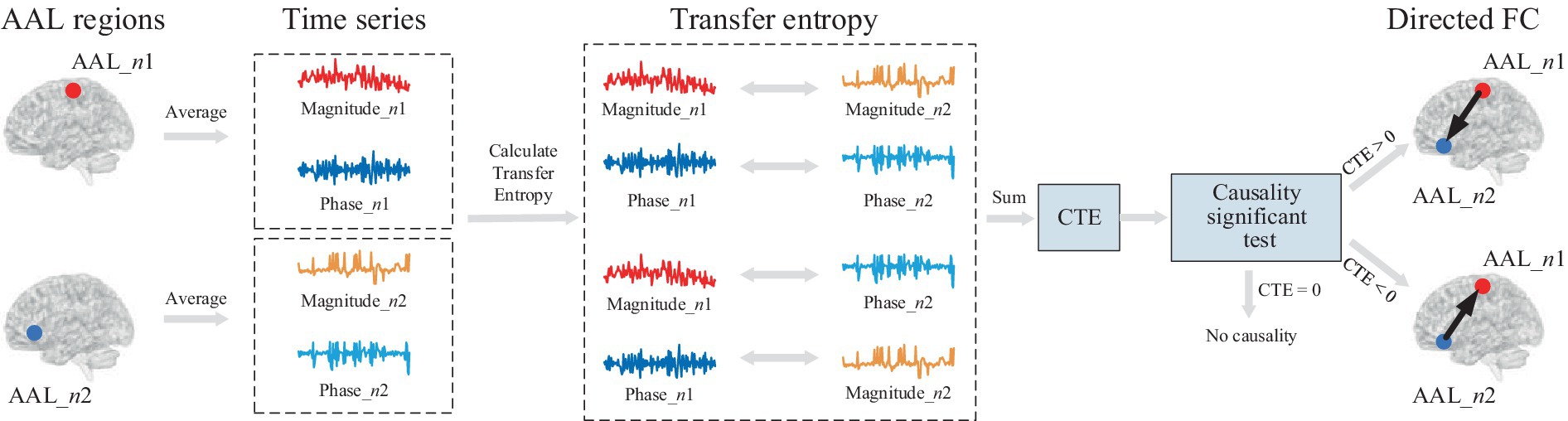
Figure 1. Framework diagram for directed FC measured by CTE. First, average complex-valued time series from two AAL regions are obtained. Each average time series involves magnitude and phase. To quantify complete complex-valued causality, CTE considers four parts of causality, including magnitude–magnitude, phase–phase, and two magnitude–phase causality. After the causal significant test, the directed FC between two regions is measured by CTE.

We denote two complex-valued signals as $z_1=\left\{z_1\left(t\right)\right\}={\left[z_1\left(1\right),\dots ,z_1\left(T\right)\right]}^{\mathrm{T}}$, $z_2=\left\{z_2\left(t\right)\right\}={\left[z_2\left(1\right),\dots ,z_2\left(T\right)\right]}^{\mathrm{T}}$, $t=1,\dots ,T$, and T is the data length. The two signals are represented with magnitude and phase in Eq. (1) as follows:

$\begin{array}{cc}{z}_1& =a\exp \left(j\theta \right)\\ z_2& =b\exp \left(j\phi \right)\end{array}\text{ (1)}$

where $a\in {ℝ}^T$ and $\theta \in {ℝ}^T$ are the magnitude and phase of $z_1$, and $b\in {ℝ}^T$ and $\phi \in {ℝ}^T$ are the magnitude and phase of $z_2$.

Based on the relationship between the magnitude and phase of the brain networks (Yu et al., 2015), we propose a definition of CTE considering complete causality between two complex-valued signals. Motivated by the complex-valued mutual information introduced by Goebel et al. (2011), CTE combines the magnitude and phase to make causality inference and is represented as follows:

$\begin{array}{c}{\mathcal{C}}_{z1\to z2}={\mathcal{R}}_{a\to b}+{\mathcal{R}}_{\theta \to \phi }+{\mathcal{R}}_{a\to b|\theta }+{\mathcal{R}}_{\theta \to \phi |a}\end{array}\text{ (2)}$

where ${\mathcal{R}}_{a\to b}$ and ${\mathcal{R}}_{\theta \to \phi }$ are real-valued transfer entropy from the magnitude and the phase of the two signals, respectively. ${\mathcal{R}}_{a\to b|\theta }$ and ${\mathcal{R}}_{\theta \to \phi |a}$ are partial transfer entropy (Papana et al., 2012), which extends transfer entropy to account for the presence of the third variable. We extend to quantify the complementary phase and magnitude effects on the causality ${\mathcal{R}}_{a\to b}$ and ${\mathcal{R}}_{\theta \to \phi }.$

Real-valued transfer entropy ${\mathcal{R}}_{a\to b}$ and ${\mathcal{R}}_{\theta \to \phi }$ in Eq. (2) can be calculated as follows (Schreiber, 2000):

$\begin{array}{c}\begin{array}{cc}{\mathcal{R}}_{a\to b}& =\sum p\left(b_t,b_{t-\tau },a_{t-\tau }\right)\log \frac{p\left(b_t|b_{t-\tau },a_{t-\tau }\right)}{p\left(b_t|b_{t-\tau }\right)}\\ {\mathcal{R}}_{\theta \to \phi }& =\sum p\left({\phi }_t,{\phi }_{t-\tau },{\theta }_{t-\tau }\right)\log \frac{p\left({\phi }_t|{\phi }_{t-\tau },{\theta }_{t-\tau }\right)}{p\left({\phi }_t|{\phi }_{t-\tau }\right)}\end{array}\end{array}\text{ (3)}$

where $a\to b$ denotes causal direction from $a$ to $b$, $p(\cdot )$ is a marginal probability density function, ${}^{"}p{\left(\cdot |\cdot \right)}^{"}$ represents a condition probability density function, $\tau$ is the parameter of time delay, and $a_{t-\tau }$ and $b_{t-\tau }$ are delayed $a$ and $b$ by $\tau$ time points. By calculating the Pearson correlation coefficient between the two signals with different time delays, the time delay corresponding to the maximum correlation coefficient is selected as the value of $\tau$.

Real-valued partial transfer entropy ${\mathcal{R}}_{a\to b|\theta }$ in Eq. (2) is determined as follows:

$\begin{array}{c}{\mathcal{R}}_{a\to b|\theta }=-\sum p\left(b_t|b_{t-\tau },{\theta }_{t-\tau }\right)\log \left\{p\left(b_t|b_{t-\tau },{\theta }_{t-\tau }\right)\right\}\\ +\sum p\left(b_t|a_{t-\tau },b_{t-\tau },{\theta }_{t-\tau }\right)\log \left\{p\left(b_t|a_{t-\tau },b_{t-\tau },{\theta }_{t-\tau }\right)\right\}\end{array}\text{ (4)}$

In Eq. (4), it can be observed that phase $\theta$ and magnitude $a$ are jointly used to determine the causal direction to magnitude $b$. In other words, ${\mathcal{R}}_{a\to b|\theta }$ incorporates magnitude–phase causality between $\theta$ and $b$ by quantifying the complementary magnitude effects of $a$ on the causality. Similarly, ${\mathcal{R}}_{\theta \to \phi |a}$ can be calculated as follows:

$\begin{array}{c}{\mathcal{R}}_{\theta \to \phi |a}=-\sum p\left({\phi }_t|a_{t-\tau },{\phi }_{t-\tau }\right)\log \left\{p\left({\phi }_t|a_{t-\tau },{\phi }_{t-\tau }\right)\right\}\\ +\sum p\left({\phi }_t|{\theta }_{t-\tau },{\phi }_{t-\tau },a_{t-\tau }\right)\log \left\{p\left({\phi }_t|{\theta }_{t-\tau },{\phi }_{t-\tau },a_{t-\tau }\right)\right\}\end{array}\text{ (5)}$

In Eqs. (2)–(5), we need to estimate condition probability density functions and joint probability density functions. We represent the condition probability density function with joint probability density functions and then estimate joint probability density functions. Taking $p\left(b_t|b_{t-\tau },{\theta }_{t-\tau }\right)$ as an example, we have the following:

$\begin{array}{c}p\left(b_t|b_{t-\tau },{\theta }_{t-\tau }\right)=\frac{p\left({\theta }_{t-\tau },b_{t-\tau },b_t\right)}{p\left({\theta }_{t-\tau },b_{t-\tau }\right)}\end{array}\text{ (6)}$

where $p\left({\theta }_{t-\tau },b_{t-\tau },b_t\right)$ and $p\left({\theta }_{t-\tau },b_{t-\tau }\right)$ are joint probability density functions. To estimate the joint probability density functions, we perform symbolic processing on each of the variables. The symbolic process helps to improve the noise robustness to traditional transfer entropy and helps capture more non-linear causality proved by the previous study (Gu et al., 2021). Taking the phase $\theta ={\left[\theta \left(1\right),\dots ,\theta \left(T\right)\right]}^{\mathrm{T}}$ as an example, where superscript “T” represents the matrix transpose, the symbolic $\theta \left(t\right)$, $1\le t\le T$, denoted as ${\theta }^{\ast }\left(t\right)$ is computed as follows (Wessel et al., 2000):

$\begin{array}{c}{\theta }^{\ast }\left(t\right)=\{\begin{array}{l}\begin{array}{cc}0:& {\mu }_p<\theta \left(t\right)\le \left(1+\beta \right){\mu }_p\end{array}\hfill \\ \begin{array}{c}\begin{array}{cc}1:& \left(1+\beta \right){\mu }_p<\theta \left(t\right)<\infty \end{array}\\ \begin{array}{c}\begin{array}{ll}2:\hfill & \left(1-\beta \right){\mu }_p<\theta \left(t\right)\le {\mu }_p\hfill \end{array}\\ \begin{array}{cc}3:& 0\le \theta \left(t\right)\le \left(1-\beta \right){\mu }_p\end{array}\end{array}\end{array}\hfill \end{array},if\theta \left(t\right)\ge 0\end{array}\text{ (7)}$

$\begin{array}{c}{\theta }^{\ast }\left(t\right)=\{\begin{array}{l}\begin{array}{cc}0:& \left(1+\beta \right){\mu }_n\le \theta \left(t\right)<{\mu }_n\end{array}\hfill \\ \begin{array}{c}\begin{array}{cc}1:& -\infty <\theta \left(t\right)<\left(1+\beta \right){\mu }_n\end{array}\\ \begin{array}{c}\begin{array}{ll}2:\hfill & {\mu }_n\le \theta \left(t\right)<\left(1-\beta \right){\mu }_n\hfill \end{array}\\ \begin{array}{cc}3:& \left(1-\beta \right){\mu }_n\le \theta \left(t\right)<0\end{array}\end{array}\end{array}\hfill \end{array},if\theta \left(t\right)<0\end{array}\text{ (8)}$

where $\beta$ is a control parameter and set to be 0.05 according to the previous study (Wessel et al., 2000), and ${\mu }_p$ and ${\mu }_n$ are the mean of positive and negative variables of $\theta ,$ respectively. As such, we obtain the symbolic variable vector of $\theta$ as ${\theta }^{\ast }={\left[{\theta }^{\ast }\left(1\right),\dots ,{\theta }^{\ast }\left(T\right)\right]}^{\mathrm{T}}.$ For simplicity, superscript “*” is omitted. $\phi$ can be symbolized in the same way. Magnitude $a$, $b$ is symbolized only using Eq. (7) with non-negative values.

Then, we exploit a histogram-based method to estimate the joint probability density function by counting the number of common elements in segmented bins between vectors. Take $p\left({\theta }_{t-\tau },b_{t-\tau }\right)$ in Eq. (6), for example, ${\theta }_{t-\tau }$ is divided into $k_{\theta }$ equal bins with the bin index denoted as i, and $b_{t-\tau }$ is divided into $k_{\theta }$ equal bins with the bin index as j. Denoting the segmented bin of ${\theta }_{t-\tau }$ and $b_{t-\tau }$ as $\mathrm{\Delta }\theta$ and $\mathrm{\Delta }b,$ the joint probability density function $p\left({\theta }_{t-\tau },b_{t-\tau }\right)$ is estimated by counting the elements number of ${\theta }_{t-\tau }$ and $b_{t-\tau }$ within the segmented bin $[\mathrm{\Delta }\theta ,\mathrm{\Delta }b].$ The parameters of bin width $\mathrm{\Delta }\theta$ and $\mathrm{\Delta }b$ are determined by the number of segmented bins and data length. For simplicity, the parameters $\mathrm{\Delta }\theta$ or $\mathrm{\Delta }b$ are equal and can be selected as follows:

$\begin{array}{c}\mathrm{\Delta }\theta =\frac{\max \left\{\left[{\theta }_{t-\tau }\mathrm{;}{b}_{t-\tau }\right]\right\}-\min \left\{\left[{\theta }_{t-\tau }\mathrm{;}{b}_{t-\tau }\right]\right\}}{T}\end{array}\text{ (9)}$

Thus, the joint probability density function $p\left({\theta }_{t-\tau },b_{t-\tau }\right)$ located around the point $\left(i,j\right)$ is represented as follows:

$\begin{array}{c}p\left({\theta }_{t-\tau },b_{t-\tau }\right)=\frac{num\left(i,j\right)}{T-\tau }\end{array}\text{ (10)}$

where $num\left(\mathrm{\Delta }\theta ,\mathrm{\Delta }b\right)$ is the number of elements between ${\theta }_{t-\tau }$ and $b_{t-\tau }$ within the segmented bin $[\mathrm{\Delta }\theta ,\mathrm{\Delta }b]$ around $\left(i,j\right)$.

2.2 Significance test of causality

The complex-valued transfer entropy ${\mathcal{C}}_{z1\to z2}$ quantifies causality from $z_1$ to $z_2$ but cannot measure the significance of the causality. As such, we define the causality significance using a statistical test together with a shuffling strategy, which has been previously used in real-valued transfer entropy studies (Bossomaier et al., 2016). The shuffling process assists in eliminating spurious causality between $z_1$ and $z_2$, ensuring the stability and accuracy of the causality measurement. Various transfer entropy differences between the original and shuffled signals are obtained by repeating the shuffling process (R times). Here, the number of times we perform shuffling, i.e., R, is set to 100. Then, one-sample t-test on the R causality differences is performed to detect the causality significance from $z_1$ to $z_2$.

If we denote the shuffled transfer entropy as ${\mathcal{C}}_{z1\to z2}^{\text{shuffled}}$, the transfer entropy difference ${\mathcal{C}}_{z1\to z2}^{\ast }$ is obtained in Eq. (11) as follows:

$\begin{array}{c}{\mathcal{C}}_{z1\to z2}^{\ast }={\mathcal{C}}_{z1\to z2}-{\mathcal{C}}_{z1\to z2}^{\text{shuffled}}\end{array}\text{ (11)}$

Similarly, ${\mathcal{C}}_{z2\to z1}^{\ast }$ is obtained in Eq. (12) as follows:

$\begin{array}{c}{\mathcal{C}}_{z2\to z1}^{\ast }={\mathcal{C}}_{z2\to z1}-{\mathcal{C}}_{z2\to z1}^{\text{shuffled}}\end{array}\text{ (12)}$

Let $\mathrm{\Delta }\mathcal{C}={\mathcal{C}}_{z1\to z2}^{\ast }-{\mathcal{C}}_{z2\to z1}^{\ast },$ $\mathrm{\Delta }\mathcal{C}={\left[\mathrm{\Delta }{\mathcal{C}}^{\left(1\right)},\dots ,\mathrm{\Delta }{\mathcal{C}}^{\left(R\right)}\right]}^{\mathrm{T}}$ includes all the transfer entropy differences between ${\mathcal{C}}_{z1\to z2}^{\ast }$ and ${\mathcal{C}}_{z2\to z1}^{\ast }$, we perform one sample t-test with the false discovery rate (FDR) correction as follows (Guo and Bhaskara, 2008):

$\begin{array}{c}\mathrm{\Delta }\mathcal{C}=\{\begin{array}{cc}\mathrm{\Delta }\overline{\mathcal{C}}& \mathrm{p}.\text{ttest}\left(\mathrm{\Delta }\mathcal{C}\right)<p_{\text{th}}\\ 0,& \text{otherwise}\end{array}\end{array}\text{ (13)}$

where $\mathrm{\Delta }\overline{\mathcal{C}}$ is the mean of $\mathrm{\Delta }\mathcal{C},$ $p_{\text{th}}$=0.05. We define the causal direction by the sign of $\mathrm{\Delta }\mathcal{C}$ as follows:

$\begin{array}{c}\text{sig}\_\text{causality}=\{\begin{array}{cc}{z}_1\to z_2,& \mathrm{\Delta }\mathcal{C}>0\\ z_2\to z_1,& \mathrm{\Delta }\mathcal{C}<0\\ \text{no}\text{causality},& \mathrm{\Delta }\mathcal{C}=0\end{array}\end{array}\text{ (14)}$

3 Experimental methods

3.1 Simulated signals

To evaluate the efficacy of CTE, we generate two sets of simulated complex-valued signals with linear and non-linear causality, respectively. Each set has three types of causal directions and is randomly generated 1,000 times and divided into 10 groups.

The baseline signals are generated using a widely used MATLAB toolbox named Granger causal connectivity analysis (GCCA) (Seth, 2010). The signals are generated with real-valued linear causality via an AR model as Seth (2010):

$\begin{array}{c}\begin{array}{ll}{x}_1\left(t\right)& =0.95\sqrt{2}{x}_1\left(t-1\right)-0.9025x_1\left(t-2\right)+w_1\left(t\right)\\ x_2\left(t\right)& =0.5x_1\left(t-1\right)+w_2\left(t\right)\end{array}\end{array}\text{ (15)}$

where $3\le t\le T$, T is the data length and set to be 146 to keep the same data length as in the fMRI data. $w_1\left(t\right)$ and $w_2\left(t\right)$ are random variables with zero mean and unit variance satisfying normal distribution. The linear and non-linear causality with different causality cases can be obtained by exploiting and modifying the baseline signals defined in Eq. (15).

When generating simulated signals with linear causality, the three types of simulated complex-valued signals are denoted as type L1, L2, and L3, respectively. The magnitude and phase of the two signals $z_1$ and $z_2$ from the three linear types are generated using Eqs. (16)–(18) as follows::

1.$\text{type}\mathrm{L}1$:

$\begin{array}{c}\begin{array}{ll}\hfill a\left(t\right)& =0.95\sqrt{2}a\left(t-1\right)-0.9025a\left(t-2\right)+w_1\left(t\right)\\ \hfill b\left(t\right)& =0.5a\left(t-1\right)+w_2\left(t\right)\\ \hfill \begin{array}{c}\hfill \theta \left(t\right)\\ \hfill \phi \left(t\right)\end{array}& \begin{array}{l}=0.95a\left(t\right)-0.9025a\left(t-2\right)+w_1\left(t\right)\hfill \\ =-0.6a\left(t\right)+w_2\left(t\right)\hfill \end{array}\end{array}\end{array}\text{ (16)}$

2. $\text{type}\mathrm{L}2$:

$\begin{array}{c}\begin{array}{ll}\hfill a\left(t\right)& =0.95\sqrt{2}a\left(t-1\right)-0.9025a\left(t-2\right)+w_1\left(t\right)\\ \hfill b\left(t\right)& =0.5a\left(t-1\right)+w_2\left(t\right)\\ \begin{array}{c}\hfill \theta \left(t\right)\\ \hfill \phi \left(t\right)\end{array}& \begin{array}{l}=0.95\theta \left(t\right)-0.9025\theta \left(t-2\right)+w_3\left(t\right)\hfill \\ =-0.6\theta \left(t\right)+w_4\left(t\right)\hfill \end{array}\end{array}\end{array}\text{ (17)}$

3. $\text{type}\mathrm{L}3$:

$\begin{array}{c}\begin{array}{ll}\hfill a\left(t\right)& =0.95\sqrt{2}a\left(t-1\right)-0.9025a\left(t-2\right)+w_1\left(t\right)\\ \hfill b\left(t\right)& =0.5a\left(t-1\right)+w_2\left(t\right)\\ \begin{array}{c}\hfill \theta \left(t\right)\\ \hfill \phi \left(t\right)\end{array}& \begin{array}{l}=r_1\left(t\right)\hfill \\ =r_2\left(t\right)\hfill \end{array}\end{array}\end{array}\text{ (18)}$

where $r_1\left(t\right)$ and $r_2\left(t\right)$ are randoms without causality.

The non-linear causality can be obtained by adding quadratic and three-order terms to (Eq. 15). The magnitude and phase of the three types (N1, N2, and N3) can be generated using Eqs. (19)–(21) as follows:

1. $\text{type}\mathrm{N}1$:

$\begin{array}{c}\begin{array}{ll}\hfill a\left(t\right)& =0.95\sqrt{2}a\left(t-1\right)-0.9025a\left(t-2\right)+w_1\left(t\right)\\ \hfill b\left(t\right)& =0.5a^2\left(t-1\right)+w_2\left(t\right)\\ \begin{array}{c}\hfill \theta \left(t\right)\\ \hfill \phi \left(t\right)\end{array}& \begin{array}{l}=0.95a\left(t\right)-0.9025a\left(t-2\right)+w_1\left(t\right)\hfill \\ =-0.6a^3\left(t\right)+w_2\left(t\right)\hfill \end{array}\end{array}\end{array}\text{ (19)}$

2.$\text{type}\mathrm{N}2$:

$\begin{array}{c}\begin{array}{ll}\hfill a\left(t\right)& =0.95\sqrt{2}a\left(t-1\right)-0.9025a\left(t-2\right)+w_1\left(t\right)\\ \hfill b\left(t\right)& =0.5a^2\left(t-1\right)+w_2\left(t\right)\\ \begin{array}{c}\hfill \theta \left(t\right)\\ \hfill \phi \left(t\right)\end{array}& \begin{array}{l}=0.95\theta \left(t\right)-0.9025\theta \left(t-2\right)+w_3\left(t\right)\hfill \\ =-0.6{\theta }^3\left(t\right)+w_4\left(t\right)\hfill \end{array}\end{array}\end{array}\text{ (20)}$

3.$\text{type}\mathrm{N}3$:

$\begin{array}{c}\begin{array}{ll}\hfill a\left(t\right)& =0.95\sqrt{2}a\left(t-1\right)-0.9025a\left(t-2\right)+w_1\left(t\right)\\ \hfill b\left(t\right)& =0.5a^2\left(t-1\right)+w_2\left(t\right)\\ \begin{array}{c}\hfill \theta \left(t\right)\\ \hfill \phi \left(t\right)\end{array}& \begin{array}{l}=r{}_1\left(t\right)\hfill \\ =r_2\left(t\right)\hfill \end{array}\end{array}\end{array}\text{ (21)}$

where $w_1\left(t\right)$, $w_2\left(t\right)$, $w_3\left(t\right),$ and $w_4\left(t\right)$ are variables with zero-valued mean, unit variance satisfying normal distribution, and without causality.

Figure 2 shows the ground truth causal directions for the three types of two simulated complex-valued signals with non-linear and linear causality. Specifically, type L1/N1 has the complete complex-valued causality including magnitude–magnitude, phase–phase, and magnitude–phase; type L2/N2 has the incomplete complex-valued causality including magnitude–magnitude and phase–phase; type L3/N3 only has magnitude–magnitude causality.

Figure 2

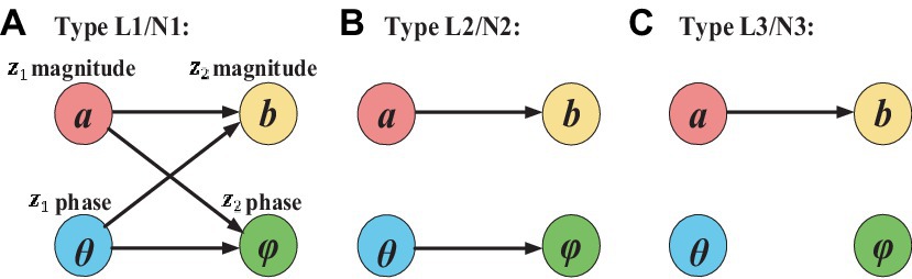
Figure 2. Ground truth casual direction for three types of simulated linear and non-linear signals. The arrow represents the causal direction.

Figure 3 presents example waveforms of simulated signals z₁ and z₂ from type L1 and type N1. The ground-truth causal direction for the magnitude and phase is shown in Figure 2A. We observe the peaks of the cause signals (z₁ magnitude and z₁ phase, in red) are ahead of the effect signals (z₂ magnitude and z₂ phase, in blue) in all cases, which are consistent with the causal direction of Figure 2. To test the noise effects on CTE, we also add Gaussian noise to the simulated signals with the signal-to-noise ratio (SNR) ranging from −10 dB to 10 dB.

Figure 3

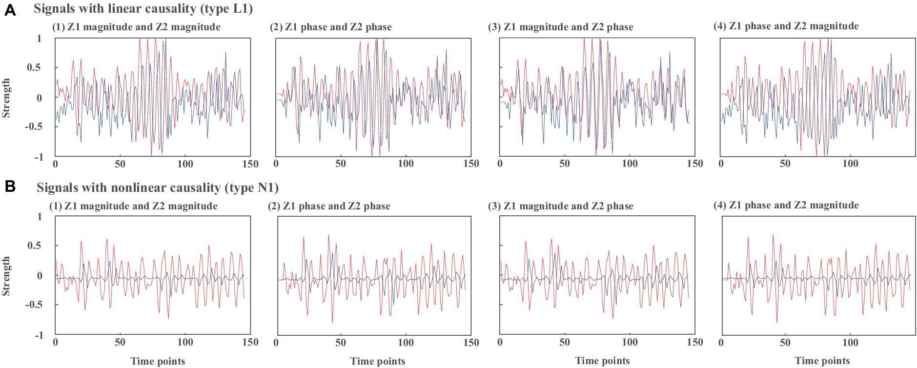
Figure 3. Waveforms of simulated signals z1 and z2 from (A) type L1 and (B) type N1. (1) z1 magnitude and z2 magnitude, (2) z1 phase and z2 phase, (3) z1 magnitude and z2 phase, (4) z1 phase and z2 magnitude.

3.2 Experimental fMRI data

The resting-state complex-valued fMRI data were a self-collected dataset from 80 subjects, including 40 healthy controls (HCs) and 40 patients with schizophrenia (SZs) with written subject consent overseen by the University of New Mexico Institutional Review Board. Specifically, there are 28 men and 12 women for HCs (mean age ± standard deviation: 36.25 ± 11.40) and 33 men and 7 women for SZs (mean age ± standard deviation: 40.73 ± 14.43). During the scan, all the participants were instructed to rest quietly in the scanner and keep their eyes open without sleeping and not to think of anything in particular (Lin et al., 2022). fMRI scans were acquired by a Siemens 3 T TIM Trio scanner equipped with a 12-channel head coil. The functional scan was acquired with the following parameters: TR = 2 s, TE = 29 ms, field of view = 24 cm, acquisition matrix = 64 × 64, flip angle = 75°, slice thickness = 3.5 mm, and slice gap = 1 mm. Data preprocessing was performed using the SPM software package.¹ Functional images were motion-corrected and then spatially normalized into the standard Montreal Neurological Institute space. Following spatial normalization, the data were resampled to 3 × 3 × 3 mm³, resulting in 53 × 63 × 46 voxels. Both magnitude and phase images were spatially smoothed with an 8 × 8 × 8 mm³ full-width half-maximum (FWHM) Gaussian kernel. Phase images were first motion corrected using the transformations computed from magnitude-only data; then, complex division of phase data by the first time point reduced the need for phase unwrapping; and spatial normalization of phase images used the warp parameters computed from magnitude-only data.

3.3 Complex-valued time series of ROI

Brodmann area (BA) and anatomical automatic labeling (AAL) atlas are two commonly used references to divide the brain into ROIs for FC analysis. Compared with BA, AAL obtains more ROIs and involves the cerebellum regions. To achieve a more comprehensive and detailed segmentation of the brain regions, we used AAL to obtain 116 ROIs (Tzourio-Mazoyer et al., 2002) and divided the 116 ROIs into 10 brain networks proposed by Smith et al. (2009), consisting of medial visual areas (MV), occipital pole visual areas (OPV), lateral visual areas (LV), default mode network (DMN), cerebellum (CER), sensorimotor (SEM), temporal lobe (TEM), anterior DMN (ADMN), left frontal parietal area (LFP), and right frontal parietal area (RFP). By dividing the 116 ROIs into these 10 networks, it is better to reveal the regularities of connections and establish relationships between FC and FNC.

The complex-valued time series for each ROI is expressed in Eq. (22) as follows:

$\begin{array}{c}{x}_n=\left|{\overline{x}}_n\left(t\right)\right|\exp \left\{j\phi \left({\overline{x}}_n\left(t\right)\right)\right\}\end{array}\text{ (22)}$

where $\left|{\overline{x}}_n\left(t\right)\right|$$\phi \left({\overline{x}}_n\left(t\right)\right),n=1,\mathrm{..},116,t=1,\mathrm{..},T$ are the averaged magnitude and phase time series across all voxels within each ROI, and T denotes the total number of time points. The causality between any two ROIs can be quantified by CTE as $\mathrm{\Delta }\mathcal{C}\left\{x_{n1},x_{n2}\right\}$ using Eqs. (2), (13), and (14).

3.4 Performance measures

In order to evaluate the proposed CTE, we compare it with the three real-valued causal analysis methods STE, HTE, and Granger, and one complex-valued approach, i.e., sCTE without considering magnitude and phase causality defined in Eq. (23) as follows:

$\begin{array}{c}{\tilde{\mathcal{C}}}_{z1\to z2}={\mathcal{R}}_{a\to b}+{\mathcal{R}}_{\theta \to \phi }\end{array}\text{ (23)}$

For the real-valued causal methods, both STE and HTE calculate real-valued TE ${\mathcal{R}}_{a\to b}$ between magnitudes in Eq. (3). Specifically, STE utilized the symbolic process in Eqs. (7) and (8) before estimating joint PDF using Eqs. (9) and (10), while HTE estimates joint PDF without symbolic process.

Granger causal test is based on utilizing linear regression models to perform a statistical causality inference. Given two variables $a$ and $b$, the autoregressive (AR) model of the Granger causal test is represented in Eq. (24) as follows:

$\begin{array}{c}\begin{array}{c}{a}_t={\displaystyle \sum _{j=1}^J}{u}_j{a}_{t-j}+{\displaystyle \sum _{j=1}^J}{v}_j{b}_{t-j}+{\epsilon }_t\\ a_t={\displaystyle \sum _{j=1}^J}{c}_j{a}_{t-j}+{\eta }_t\end{array}\end{array}\text{ (24)}$

where $u_j$, $v_j$, and $c_j$ are the regression coefficients for the model, J is the estimated time delay between $a$ and $b$, and ${\epsilon }_t$ and ${\eta }_t$ are two independent series satisfying Gaussian distribution. The fitting variances of using $a_{t-j}$, $b_{t-j}$ to fit $a_t$, and only using $a_{t-j}$ are denoted as ${\sigma }^2\left(a_t|,a_{t-j}|,b_{t-j}\right)$ and ${\sigma }^2\left(a_t|a_{t-j}\right)$, respectively. The causal direction between $a$ and $b$ is judged by comparing the fitting variance using Eq. (25) as follows:

$\begin{array}{c}b\to a,if{\sigma }^2\left(a_t|a_{t-j}\right)>{\sigma }^2\left(a_t|,a_{t-j}|,b_{t-j}\right)\end{array}\text{ (25)}$

As such, the causal direction is evaluated by Granger causality.

For simulated signals, we calculate the accuracy of directed inference in Eq. (26), denoted as AOC, as follows:

$\begin{array}{c}\text{AOC}=N_{\text{correct}}/N_{\text{total}}\end{array}\text{ (26)}$

where $N_{\text{correct}}$ is the number of correct causal direction judgments and $N_{\text{total}}$ is the total number of causality evaluations between two signals.

For experimental fMRI data, we first calculate the average Pearson correlation coefficient between the magnitude and phase from two different ROI signals in HCs or SZs, to validate magnitude and phase dependence in Eq. (27) as follows:

$\begin{array}{c}\overline{\rho }=\frac{1}{K}{\displaystyle \sum _{k=1}^K}\text{cor}\left(\left|{\overline{x}}_m^{\left(k\right)}\right|,\phi \left({\overline{x}}_n^{\left(k\right)}\right)\right),m,n=1,\dots ,116\end{array}\text{ (27)}$

Second, we perform two-sample t-tests (p_th = 0.05) on connections from HCs and SZs with the FDR correction (Guo and Bhaskara, 2008) to obtain significant intergroup differences in Eq. (28) as follows:

$\begin{array}{c}{d}_{n,m}=\{\begin{array}{cc}t\_\mathit{\text{value}}& \mathrm{p}.\text{ttest}2\left(\mathrm{\Delta }{\mathcal{C}}_{n,m}^{\left(\text{HC}\right)},\mathrm{\Delta }{\mathcal{C}}_{n,m}^{\left(\text{SZ}\right)}\right)<p_{\text{th}}\\ 0,& \text{otherwise}\end{array}\end{array}\text{ (28)}$

where n and m represent two different ROIs or two brain networks, $\mathrm{\Delta }{\mathcal{C}}_{n,m}^{\left(\text{HC}\right)}=\left[\mathrm{\Delta }{\mathcal{C}}_{n,m}^{\left(\text{HC},1\right)},\dots ,\mathrm{\Delta }{\mathcal{C}}_{n,m}^{\left(\text{HC},K\right)}\right]$ and $\mathrm{\Delta }{\mathcal{C}}_{n,m}^{\left(\text{SZ}\right)}=\left[\mathrm{\Delta }{\mathcal{C}}_{n,m}^{\left(\text{SZ},1\right)},\dots ,\mathrm{\Delta }{\mathcal{C}}_{n,m}^{\left(\text{SZ},K\right)}\right].$

Third, we compare the number of common and unique connections detected by each method. Finally, we compare the efficacy of the common and unique connections as features to classify HCs and SZs using support vector machine (SVM). The multilayer perceptron kernel is selected, and SVM is repeated 1,000 times. Given a training dataset of $K1$ subjects as $\left[\left(x_1,y_1\right),\dots ,\left(x_{K1},y_{K1}\right)\right]$, where $x_k\in {ℂ}^{M1},1\le k\le K1$ represents the connectivity vector from the kth subject, M1 is the vector length, and $y_k$ is the label denoted as either 1 or − 1, indicating which class of $x_k$ belongs to. SVM aims to find a hyperplane to maximize the distance between the dataset and the hyperplane. The hyperplane can be represented in Eq. (29) as follows:

$\begin{array}{c}f\left(x_k\right)={\omega }^{\mathrm{T}}\varphi \left(x_k\right)+b\end{array}\text{ (29)}$

where $\omega$ and $b$ are parameters of the hyperplane, and $\varphi \left(x_k\right)$ is the kernel function. Multiple kernel functions can be used, e.g., the linear kernel, quadric kernel, and sigmoid kernel. By comparing the clustering performance, we select the multilayer perceptron (MLP) kernel for SVM and there are three layers including the input, hidden, and output layers. The input is the connectivity vectors $x_k$, the non-linear activation function is $\tanh \{\cdot \},$ and the output of the MLP kernel is represented in Eq. (30) as follows (Suykens and Vandewalle, 1999):

$\begin{array}{c}\varphi \left(x_k\right)=\tanh \left\{\omega 1\cdot {\left(x_k\right)}^T\cdot x_k+b1\right\}\end{array}\text{ (30)}$

where $\mathrm{\omega }1$ and $b1$ are weights and biases and are initially set to be 1 and −1, respectively. As such, the SVM classifier is built based on MLP kernel and can be realized by MATLAB built-in function named “mlp_kernel.”

The results are evaluated in terms of accuracy (ACC), sensitivity (SEN), and specificity (SPEC) defined in Eq. (31) as follows (Lin et al., 2022):

$\begin{array}{c}\begin{array}{l}\text{ACC}=\frac{\text{TP}+\text{TN}}{\text{TP}+\text{TN}+\text{FP}+\text{FN}}\hfill \\ \text{SEN}=\frac{\text{TP}}{\text{TP}+\text{FN}}\hfill \\ \text{SPEC}=\frac{\text{TN}}{\text{TN}+\text{FP}}\hfill \end{array}\end{array}\text{ (31)}$

where TP, TN, FP, and FN denote true positive, true negative, false positive, and false negative, respectively. To mitigate overfitting and guarantee reliability, leave one out cross-validation (LOOV) is performed. Specifically, LOOV leaves out the data from one subject as test data and exploits the data from the rest of the selected subjects for training. Given that, the test data are independent of the training data in each LOOV loop. LOOV is used for cross-validation purposes, given we have limited data. As such, we repeat the validation 1,000 times.

4 Results

4.1 Simulated signals

Table 1 shows the accuracy of linear/non-linear directed inference for the three types of simulated signals without noise. Five types of directed analysis methods are compared including the proposed CTE, sCTE, and three real-valued methods: STE, HTE, and Granger. Compared with the other three transfer entropy methods (sCTE, STE, and THE), CTE obtains higher accuracy for causality inference, especially when having complete complex-valued causality (type L1/N1). Specifically, for type N1 (non-linear signals containing complete complex-valued causality), CTE achieves slightly higher accuracy than the sCTE and 18.7–85.9% higher accuracy than the three real-valued algorithms.

Table 1

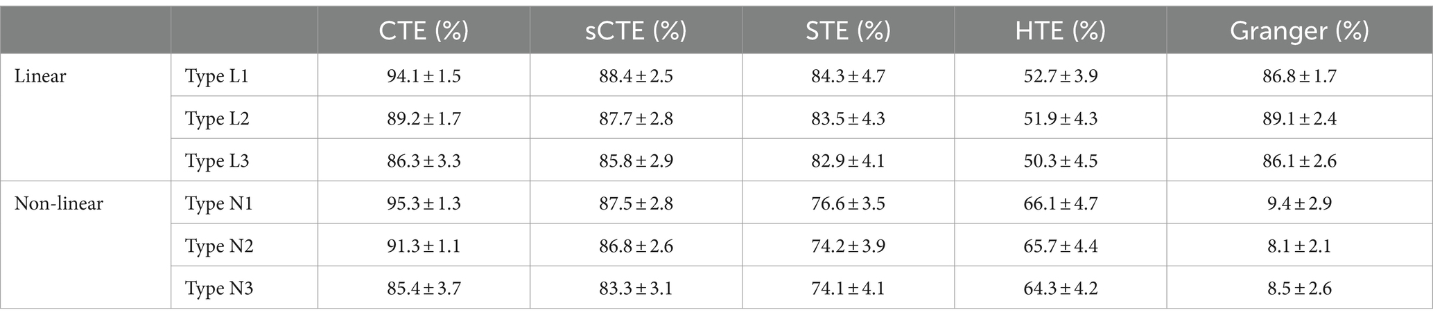
Table 1. Comparison of the mean and standard deviation of the accuracy of causality inference by five methods for simulated signals without noise.

Figure 4 shows the estimated causality accuracy for simulated signals with different SNRs. CTE achieves the highest accuracy and noise robustness for type L1/N1, due to the consideration of complete complex-valued causality. For type L2/N2, CTE and sCTE yield higher accuracy than three real-valued methods, including STE, HTE, and Granger, especially with low SNR (<-6 dB), due to the inclusion of phase causality. Regarding type L3/N3, CTE and the other transfer entropy algorithms have similar accuracy with high SNR (> 6 dB) as there only has magnitude causality. In this case, CTE is a general method suitable for measuring linear and non-linear causality for both complex-valued and real-valued signals. For type L3, note that Granger shows higher directed accuracy than CTE with SNR being -4 dB–4 dB. The reason is that Granger is built on the AR model for linear causality, making it optimal when only magnitude causality exists. However, Granger fails to detect non-linear causality. Therefore, considering both linear and non-linear scenarios, the proposed CTE is the optimal-directed algorithm in most cases.

Figure 4

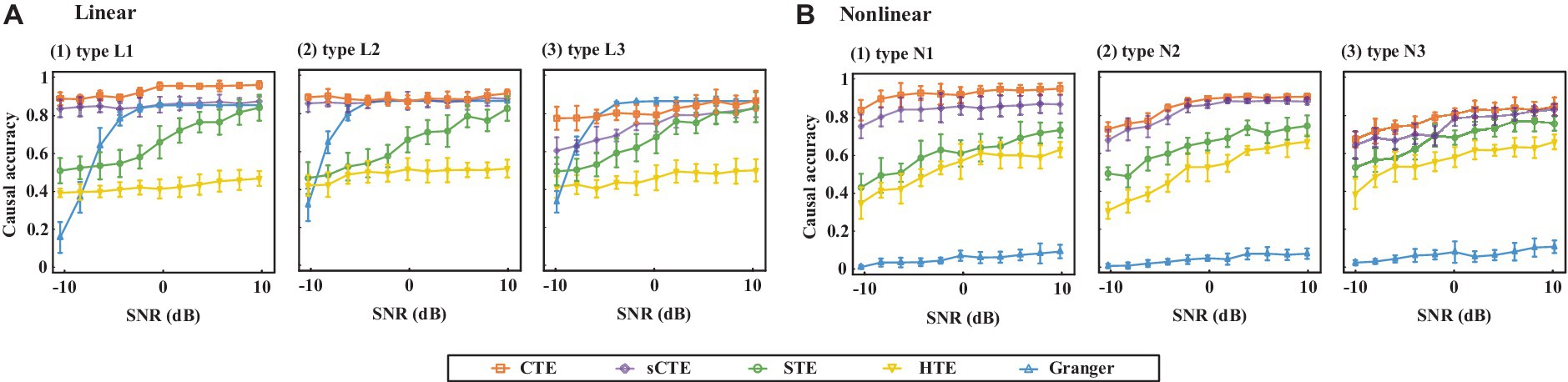
Figure 4. Causality accuracy for simulated signals with linear and non-linear causality under different SNRs.

4.2 Experimental fMRI data

After performing a two-sample t-test (p < 0.05, df = 78, FDR corrected) for the connections between HCs and SZs, we compare the numbers of common and unique connections detected by two different methods with significant HC-SZ differences. We select sCTE and STE as comparison methods since they have better performance for the simulated signals (refer to Figure 4).

Figure 5 shows the number of common and unique connections in terms of ten brain networks. In total, CTE obtains more common connections with sCTE than with STE (505 vs. 344), while detecting fewer unique connections with sCTE than with STE (105 vs. 266). The reason is that sCTE is closer to CTE by considering additional phase–phase causality relative to STE. Most of the common and unique connections belong to CER, which has been reported by previous studies to identify schizophrenia (Su et al., 2013; Watanabe et al., 2014). Other biomarker regions such as TEM, RFP, and visual areas (LV and MV) also show larger numbers of common and unique connections.

Figure 5

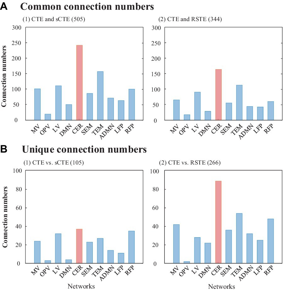
Figure 5. Common and unique connections between CTE and sCTE and between CTE and STE. The network with the maximum number of connections is highlighted in red.

Table 2 shows common and unique connections between CTE and sCTE/STE with the top five significant HCs-SZs differences. These connections are mainly related to the brain networks including CER, RFP, and TEM, which are consistent with the abnormal connections of schizophrenia obtained by previous studies (Su et al., 2013; Watanabe et al., 2014; Oestreich et al., 2016; Maher et al., 2019; Dietz et al., 2020; Rashidi et al., 2021). Moreover, CTE detects unique connections with highly significant HCs-SZs differences related to RFP (vs. sCTE), DMN, and TEM (vs. STE). Considering the numbers and t-values of the connections with significant intergroup differences in Figure 5 and Table 2, CER, TEM, and RFP may be regarded as the biomarker brain networks for identifying schizophrenia (Su et al., 2013; Nenadic et al., 2014; Watanabe et al., 2014; Oestreich et al., 2016; Zhuo et al., 2018; Rashidi et al., 2021; Sklar et al., 2021).

Table 2

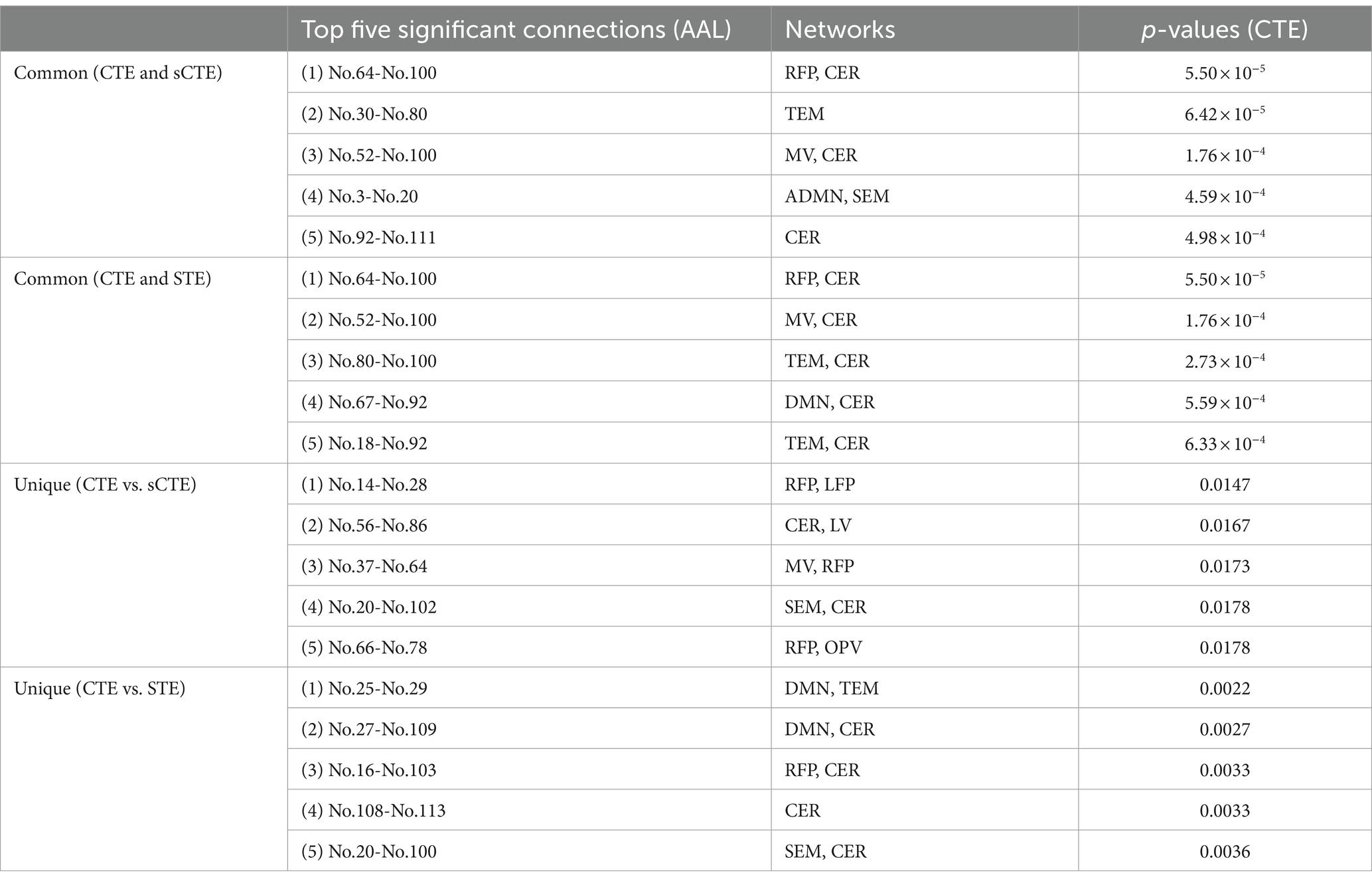
Table 2. Common and unique connections with the top five HCs-SZs significance.

Figure 6 shows the SVM classification accuracy. The features are the unique or common connections obtained by CTE, sCTE, and STE. CTE exhibits the highest accuracy (92.8%) using unique connections relative to sCTE, followed by STE. As these unique connections of CTE are mainly related to RFP and CER shown in Table 2, it suggests that RFP- and CER-related connections helps to classify HCs and SZs. After verifying CTE unique connections are helpful in classification, exploiting all the significant connections including common and unique connections for classification is evaluated in Table 3.

Figure 6

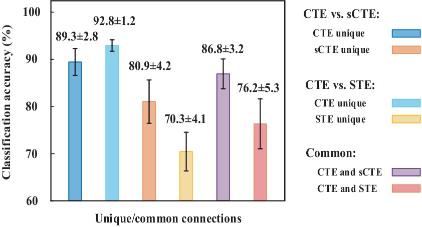
Figure 6. SVM classification accuracy for using unique/common connections obtained by CTE, sCTE, and STE, respectively. Unique connections of CTE achieve higher accuracy than others.

Table 3

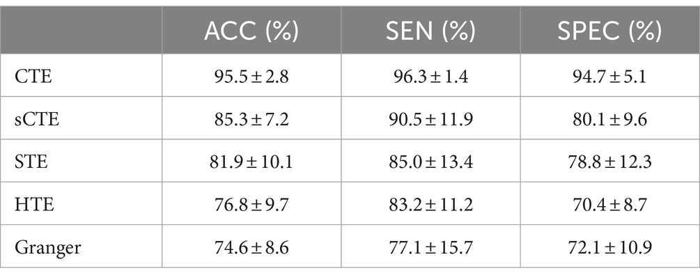
Table 3. SVM classification is performed by combining unique connections and common connections.

For all the connections with significant intergroup differences, Table 3 shows the SVM performance measures (ACC, SEN, and SPEC) from five causality algorithms. As expected, the proposed complex-valued transfer entropy methods (CTE and sCTE) achieve better performance than real-valued directed analysis methods. CTE shows the best classification performance among all the five directed analysis methods; e.g., it improves higher ACC with 10.2% (95.5% vs. 85.3%) to sCTE, 13.6% (95.5% vs. 81.9%) to STE, 18.7% (95.5% vs. 76.8%) to HTE, and 20.9% (95.5% vs. 74.6%) to Granger, respectively. The proposed CTE obtains all the highest values of the three classification measures, especially for SEN reaching to 96.3%. This suggests that CTE captures meaningful and discriminative features to identify HCs and SZ.

Several studies have employed SVM for classifying HCs and SZs, especially using FC as features. In terms of using SVM for HCs and SZs classification, we select the previous studies with similar data sizes of the dataset in the paper (40 HCs and 40 SZs) for comparison. Su et al. (2013) performed SVM to FC quantified by an extended maximal information coefficient and obtained 82.8% clustering accuracy (32 HCs and 32 SZs). By analyzing the coherence regional homogeneity value, Liu et al. (2018) demonstrated that the abnormal connections related to TEM, insula, precentral gyrus, and precuneus can be used as psychosis biomarker of schizophrenia and achieved 89.9% accuracy (31 HCs and 48 SZs). Following this, Bae et al. (2018) pointed to decreased connections in the global and local network connectivity in SZs compared with HCs, especially in DMN, left parietal region, and TEM with an accuracy of 92.1% (31 HCs and 48 SZs). Instead of using FC of magnitude data for classification, Li et al. (2024) utilized dynamic connectivity features of phase maps as features for classification and obtained 87.5% accuracy (24 HCs and 24 SZs). As mentioned above, the existing studies of real-valued connections achieved 82.8–92.1% SVM accuracy for classifying HCs and SZs. Due to making full use of both magnitude and phase fMRI data, directed FC quantified by CTE shows higher classifying accuracy (95.5%) than the previous studies with similar data sizes.

5 Discussion

To our knowledge, few studies have explored directed FC based on complex-valued fMRI data, although directed FC has been increasingly studied using magnitude-only fMRI data. In this study, we propose a non-linear complex-valued directed analysis method based on transfer entropy to make full use of complex-valued fMRI data in highlighting differences between HCs and SZs. Simulated results show that our method has the highest accuracy and noisy robustness, especially for the non-linear model with complete complex-valued causality containing magnitude–magnitude, phase–phase, and magnitude–phase relationship. Experimental results show that CTE detects more unique connections with higher significant intergroup differences, thus leading to better performance in classifying HCs and SZs.

Instead of directly quantifying magnitude–phase causality, we propose to introduce partial transfer entropy to exploit the complementary phase/magnitude effects on magnitude–phase and phase–magnitude causality. This is because partial CTE can simultaneously utilize both magnitude and phase to assess causality in Eqs. (4) and (5), while transfer entropy only considers magnitude–phase or phase–magnitude dependence without the complementary phase/magnitude effects in Eqs. (32) and (33) as follows:

$\begin{array}{c}{\mathcal{R}}_{b\to \theta }=\sum p\left(\theta ,{\theta }_{t-\tau },b_{t-\tau }\right)\log \frac{p\left({\theta }_t|{\theta }_{t-\tau },b_{t-\tau }\right)}{p\left({\theta }_t|{\theta }_{t-\tau }\right)}\end{array}\text{ (32)}$

$\begin{array}{c}{\mathcal{R}}_{a\to \phi }=\sum p\left({\phi }_t,{\phi }_{t-\tau },a_{t-\tau }\right)\log \frac{p\left({\phi }_t|{\phi }_{t-\tau },a_{t-\tau }\right)}{p\left({\phi }_t|{\phi }_{t-\tau }\right)}\end{array}\text{ (33)}$

As such, we use transfer entropy ${\mathcal{R}}_{b\to \theta }$ and ${\mathcal{R}}_{a\to \phi }$ to replace partial entropy ${\mathcal{R}}_{a\to b|\theta }$ and ${\mathcal{R}}_{\theta \to \phi |a}$ for comparison when calculating the proposed CTE.

Figure 7 shows directed accuracy for the simulated signals with linear and non-linear complete complex-valued causality (type L1 and N1). It presents that using partial transfer entropy (shorted as partial TE) to measure the complementary phase and magnitude effects on magnitude–phase causality shows better performance than those directly quantifying magnitude–phase causality using transfer entropy (TE), especially for quantifying the linear causality. When measuring the causality between magnitude and phase, partial TE considers more information, thus partial TE enhancing CTE noise robustness. It verifies the effectiveness of introducing partial TE in the proposed CTE definition.

Figure 7

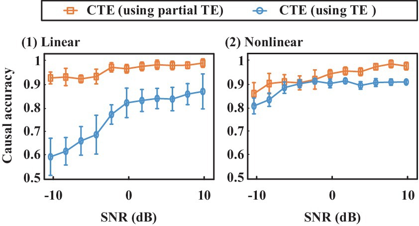
Figure 7. Causal inference accuracy comparison for CTE that using partial transfer entropy (shorted as partial TE) and TE, respectively. The proposed CTE using partial TE shows higher accuracy than the CTE that uses TE to directly quantify magnitude–phase causality.

To evaluate the data length effects on CTE, we change the simulated data length from 100 to 1,000 time points. CTE can keep high causality inference accuracy, especially for the signals with complete complex-valued causality (type L1 and N1). Because CTE keeps high causality inference accuracy to different data lengths, we can combine CTE and a sliding window approach for dynamic analysis. By performing causality analysis on the segmented time series, directed FC from different windows can be obtained. As such, dynamic statistical analysis can be exploited to analyze dynamics from the directed FC.

Figure 8 shows the average Pearson correlation coefficients between magnitude and phase from two different ROI signals across all the subjects in each group. The magnitude–phase correlation coefficients range from −0.2 to 0.2. This supports the magnitude–phase causality considered in the proposed method. Specifically, CER-related connections are marked with black boxes and locally magnified. There are polarity and strength differences between HCs and SZs in both magnitude–phase and phase–magnitude correlation coefficients. This suggests that the proposed complex-valued transfer entropy considering causality between magnitude–phase and phase–magnitude is essential and can capture more intergroup differences.

Figure 8

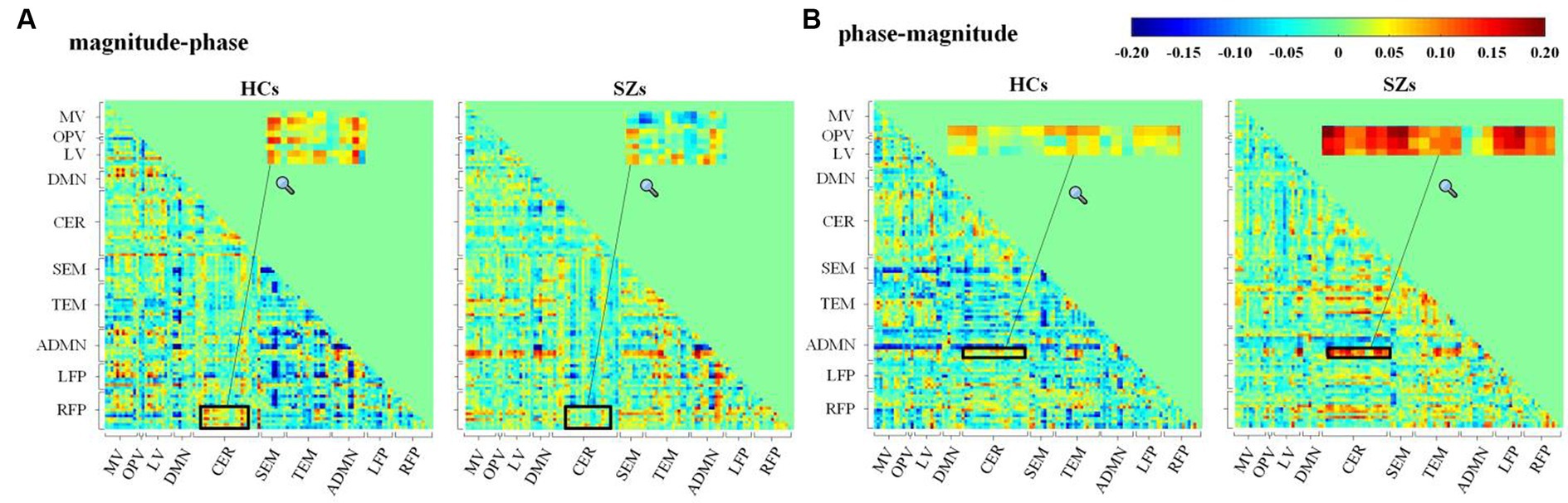
Figure 8. Average Pearson’s correlation coefficients for (A) magnitude–phase and (B) phase–magnitude of complex-valued time series from 116 AAL ROIs across subjects in HCs or SZs.

CER-related connections show more and higher significant intergroup differences obtained by the proposed CTE. Although the cerebellum has been reported to be associated with the motor system, a growing number of studies have found that the cerebellum is critical to processing complex functions, e.g., attention, cognition, and language (Lungu et al., 2013). Lungu et al. reviewed 234 fMRI studies published from 1997 to 2010 related to SZs and pointed out that 41.02% of the articles reported cerebellar activity related to cognitive, emotional, and executive processes in schizophrenia. In conclusion, the results of their analyses suggest that the cerebellum plays an essential functional role in schizophrenia, especially in the cognitive and executive domains. Following this, we performed searches in the abstracts of articles indexed in Scopus from 2011 to 2023 and found 218 articles that reported abnormal cerebellum-related connections in schizophrenia. These studies proved that the cerebellum is a functional hub involved in cognition, language, and emotional processing with regions, including TEM, DMN, and visual areas. For instance, Table 2 highlights Cerebelum_6_R (AAL No.100) has connections with significant HC-SZ difference, which is also consistent with previous studies. Su et al. (2013) quantified non-linear undirected connections and pointed out that cerebellum-related ROIs, especially CRBL6.R, were important in identifying schizophrenia. Zhuo et al. (2018) calculated FC density to investigate cerebellar connectivity changes of SZs and found abnormal connectivity strength of Cerebelum_6_R with visual areas (Zhuo et al., 2018).

Apart from CER, CTE also detects common connections related to visual areas (MV and LV), and temporal lobe (TEM) in Table 2. These two nodes have brain functions of vision and auditory, respectively. As hallucinations are a frequent symptom of schizophrenia including visual and auditory hallucinations occupying 70% of patients with schizophrenia (Demirci et al., 2008), it is expected that MV and TEM are schizophrenia-related in terms of pathology mechanisms (Fogelson et al., 2014; Dietz et al., 2020). For unique connections detected by CTE in Table 3, abnormal connectivity mainly related to RFP is verified by previous studies. Frontal parietal regions have been shown involved in the cognitive and perceptive process (Smith et al., 2009) and are highly related to the impaired cognitive function of SZs (Roiser et al., 2013). Roiser et al. pointed out that connective abnormality related to the frontal–parietal areas may link to cognitive impairment for SZs (Roiser et al., 2013), given that the unique abnormal connectivity patterns obtained by CTE may provide additional evidence for the cognitive and perceptive impairments of schizophrenia.

In addition to FC between ROI, CTE can also measure the FNC of brain networks. We use CTE to quantify the FNC of brain networks. Table 4 shows the SVM performance of the five directed analysis methods. Similar to FC results, CTE also shows the best performance among these methods. Compared with other directed analysis methods, CTE shows better classification performance, e.g., improves higher accuracy with 5.1% (88.2% vs. 83.1%) to sCTE, 9.9% (88.2% vs. 78.3%) to STE, 17.5% (88.2% vs. 70.7%) to HTE, and 16.9% (88.2% vs. 71.3%) to HTE, respectively.

Table 4

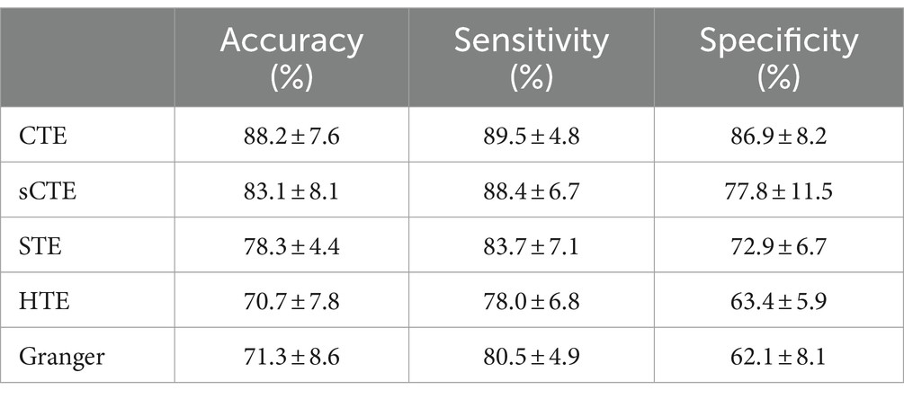
Table 4. SVM classification is performed based on the directed FNC of brain networks.

In future, our CTE approach can be extended to analyzing causal FNC of time courses extracted by blind source separation, e.g., ICA, sparse representation, and tensor decomposition. Second, dynamic-directed FC/FNC can be performed to further improve classification performance. Finally, CTE can be exploited for other mental disorders such as depressive disorder or further extended to other applications for evaluating complex-valued causality.

Data availability statement

The original contributions presented in the study are included in the article/supplementary material, further inquiries can be directed to the corresponding authors.

Ethics statement

The studies involving humans were approved by University of New Mexico Institutional Review Board. The studies were conducted in accordance with the local legislation and institutional requirements. The participants provided their written informed consent to participate in this study. Written informed consent was obtained from the individual(s) for the publication of any potentially identifiable images or data included in this article.

Author contributions

W-XL: Conceptualization, Investigation, Methodology, Software, Writing – original draft, Writing – review & editing. Q-HL: Funding acquisition, Validation, Writing – review & editing. C-YZ: Methodology, Validation, Writing – review & editing. YH: Conceptualization, Validation, Writing – review & editing. VC: Data curation, Funding acquisition, Investigation, Validation, Writing – review & editing.

Funding

The author(s) declare that financial support was received for the research, authorship, and/or publication of this article. This study was supported in part by the National Natural Science Foundation of China under Grant 61871067, in part by the NSF under Grant 2112455, in part by the NIH Grant R01MH123610, in part by the Fundamental Research Funds for the Central Universities, China, under Grant DUT20ZD220, and in part by the Supercomputing Center of Dalian University of Technology.

Conflict of interest

The authors declare that the research was conducted in the absence of any commercial or financial relationships that could be construed as a potential conflict of interest.

The reviewer L-DK declared a past co-authorship with the authors Q-HL and VC to the handling editor.

The author(s) declared that they were an editorial board member of Frontiers, at the time of submission. This had no impact on the peer review process and the final decision.

Publisher’s note

All claims expressed in this article are solely those of the authors and do not necessarily represent those of their affiliated organizations, or those of the publisher, the editors and the reviewers. Any product that may be evaluated in this article, or claim that may be made by its manufacturer, is not guaranteed or endorsed by the publisher.

Footnotes

1. ^Available at: http://www.fil.ion.ucl.ac.uk/spm.

References

Adali, T., and Calhoun, V. D. (2007). Complex ICA of brain imaging data. IEEE ASSP Mag. 24, 136–139. doi: 10.1109/SP.2007.904742

Crossref Full Text | Google Scholar

Bae, Y., Kumarasamy, K., Ali, I. M., Korfiatis, P., Akkus, Z., and Erickson, B. J. (2018). Differences between schizophrenic and normal subjects using network properties from fMRI. J. Digit. Imaging 31, 252–261. doi: 10.1007/s10278-017-0020-4

PubMed Abstract | Crossref Full Text | Google Scholar

Bastos, A. M., and Schoffelen, J. M. (2016). A tutorial review of functional connectivity analysis methods and their interpretational pitfalls. Front. Syst. Neurosci. 9:175. doi: 10.3389/fnsys.2015.00175

PubMed Abstract | Crossref Full Text | Google Scholar

Bastos-Leite, A. J., Ridgway, G. R., Silveira, C., Norton, A., Reis, S., and Friston, K. J. (2015). Dysconnectivity within the default mode in first-episode schizophrenia: a stochastic dynamic causal modeling study with functional magnetic resonance imaging. Schizophr. Bull. 41, 144–153. doi: 10.1093/schbul/sbu080

PubMed Abstract | Crossref Full Text | Google Scholar

Behrendt, S., Dimpfl, T., Peter, F. J., and Zimmermann, D. J. (2019). RTransferEntropy-quantifying information flow between different time series using effective transfer entropy. SoftwareX 10:100265. doi: 10.1016/j.softx.2019.100265

Crossref Full Text | Google Scholar

Bielczyk, N. Z., Uithol, S., van Mourik, T., Anderson, P., Glennon, J. C., and Buitelaar, J. K. (2019). Disentangling causal webs in the brain using functional magnetic resonance imaging: a review of current approaches. Netw. Neurosci. 3, 237–273. doi: 10.1162/netn_a_00062

PubMed Abstract | Crossref Full Text | Google Scholar

Bossomaier, T., Barnett, L., Harré, M., and Lizier, J. T. (2016). An introduction to transfer entropy: Information flow in complex systems. Berlin: Springer.

Google Scholar

Calhoun, V. D., Adalı, T. G., Pearlson, D., van Zijl, P. C. M., and Pekar, J. J. (2002). Independent component analysis of fMRI data in the complex domain. Magn. Reson. Med. 48, 180–192. doi: 10.1002/mrm.10202

Crossref Full Text | Google Scholar

Caserini, N. A., and Pagnottoni, P. (2022). Effective transfer entropy to measure information flows in credit markets. JISS 31, 729–757. doi: 10.1007/s10260-021-00614-1

Crossref Full Text | Google Scholar

Crimi, A., Dodero, L., Sambataro, F., Murino, V., and Sona, D. (2021). Structurally constrained effective brain connectivity. NeuroImage 239:118288. doi: 10.1016/j.neuroimage.2021.118288

Crossref Full Text | Google Scholar

Demirci, O., Clark, V. P., Magnotta, V. A., Andreasen, N. C., Lauriello, J., Kiehl, K. A., et al. (2008). A review of challenges in the use of fMRI for disease classification/characterization and a projection pursuit application from a multi-site fMRI schizophrenia study. Brain Imaging Behav. 2, 207–226. doi: 10.1007/s11682-008-9028-1

Crossref Full Text | Google Scholar

Demirci, O., Stevens, M. C., Andreasen, N. C., Michael, A., Liu, J., White, T., et al. (2009). Investigation of relationships between fMRI brain networks in the spectral domain using ICA and granger causality reveals distinct differences between schizophrenia patients and healthy controls. NeuroImage 46, 419–431. doi: 10.1016/j.neuroimage.2009.02.014

PubMed Abstract | Crossref Full Text | Google Scholar

Dietz, M. J., Zhou, Y., Veddum, L., Frith, C. D., and Bliksted, V. F. (2020). Aberrant effective connectivity is associated with positive symptoms in first-episode schizophrenia. NeuroImage 28:102444. doi: 10.1016/j.nicl.2020.102444

PubMed Abstract | Crossref Full Text | Google Scholar

Fogelson, N., Litvak, V., Peled, A., Fernandez-del-Olmo, M., and Friston, K. (2014). The functional anatomy of schizophrenia: a dynamic causal modeling study of predictive coding. Schizophr. Res. 158, 204–212. doi: 10.1016/j.schres.2014.06.011

PubMed Abstract | Crossref Full Text | Google Scholar

Friston, K. J., Preller, K. H., Mathys, C., Cagnan, H., Heinzle, J., Razi, A., et al. (2019). Dynamic causal modelling revisited. NeuroImage 199, 730–744. doi: 10.1016/j.neuroimage.2017.02.045

PubMed Abstract | Crossref Full Text | Google Scholar

Goebel, B., Essiambre, R. J., Kramer, G., Winzer, P. J., and Hanik, N. (2011). Calculation of mutual information for partially coherent Gaussian channels with applications to fiber optics. IEEE Trans. Inf. Theory 57, 5720–5736. doi: 10.1109/TIT.2011.2162187

Crossref Full Text | Google Scholar

Gu, D., Mi, Y., and Lin, A. (2021). Application of time-delay multiscale symbolic phase compensated transfer entropy in analyzing cyclic alternating pattern (CAP) in sleep-related pathological data. Commun. Nonlinear Sci. Numer. Simul. 99:105835. doi: 10.1016/j.cnsns.2021.105835

Crossref Full Text | Google Scholar

Guo, W., and Bhaskara, R. M. (2008). On control of the false discovery rate under no assumption of dependency. J. Stat. Plan Inference 138, 3176–3188. doi: 10.1016/j.jspi.2008.01.003

Crossref Full Text | Google Scholar

Jizba, P., Lavička, H., and Tabachová, Z. (2022). Causal inference in time series in terms of Rényi transfer entropy. Entropy 24:855. doi: 10.3390/e24070855

PubMed Abstract | Crossref Full Text | Google Scholar

Li, X., Coyle, D., Maguire, L., McGinnity, T. M., and Benali, H. (2011). A model selection method for nonlinear system identification based fMRI effective connectivity analysis. IEEE Trans. Med. Imaging 30, 1365–1380. doi: 10.1109/TMI.2011.2116034

PubMed Abstract | Crossref Full Text | Google Scholar

Li, W.-X., Lin, Q.-H., Zhao, B.-H., Kuang, L.-D., Zhang, C.-Y., Han, Y., et al. (2024). Dynamic functional network connectivity based on spatial source phase maps of complex-valued fMRI data: application to schizophrenia. J. Neurosci. Methods 403:110049. doi: 10.1016/j.jneumeth.2023.110049

PubMed Abstract | Crossref Full Text | Google Scholar

Li, X., Marrelec, G., Hess, R. F., and Benali, H. (2010). A nonlinear identification method to study effective connectivity in functional MRI. Med. Image Anal. 14, 30–38. doi: 10.1016/j.media.2009.09.005

PubMed Abstract | Crossref Full Text | Google Scholar

Li, M. A., and Zhang, Y. Y. (2022). A brain functional network based on continuous wavelet transform and symbolic transfer entropy. Acta Electron. Sin. 50, 1600–1608. doi: 10.12263/DZXB.20210298

Crossref Full Text | Google Scholar

Lin, Q. H., Niu, Y. W., Sui, J., Zhao, W. D., Zhuo, C., and Calhoun, V. D. (2022). SSPNet: an interpretable 3D-CNN for classification of schizophrenia using phase maps of resting-state complex-valued fMRI data. Med. Image Anal. 79:102430. doi: 10.1016/j.media.2022.102430

PubMed Abstract | Crossref Full Text | Google Scholar

Liu, Y., Guo, W., Zhang, Y., Lv, L., Hu, F., Wu, R., et al. (2018). Decreased resting-state interhemispheric functional connectivity correlated with neurocognitive deficits in drug-naive first-episode adolescent-onset schizophrenia. Int. J. Neuropsychopharmacol. 21, 33–41. doi: 10.1093/ijnp/pyx095

PubMed Abstract | Crossref Full Text | Google Scholar

Liu, J., Ji, J., Xun, G., and Zhang, A. (2022). Inferring effective connectivity networks from fMRI time series with a temporal entropy-score. IEEE Trans. Neural Netw. Learn. Syst. 33, 5993–6006. doi: 10.1109/TNNLS.2021.3072149

PubMed Abstract | Crossref Full Text | Google Scholar

Lizier, J. T., Heinzle, J., Horstmann, A., Haynes, J.-D., and Prokopenko, M. (2011). Multivariate information-theoretic measures reveal directed information structure and task relevant changes in fMRI connectivity. J. Comput. Neurosci. 30, 85–107. doi: 10.1007/s10827-010-0271-2

PubMed Abstract | Crossref Full Text | Google Scholar

Lungu, O., Barakat, M., Laventure, S., Debas, K., Proulx, S., Luck, D., et al. (2013). The incidence and nature of cerebellar findings in schizophrenia: a quantitative review of fMRI literature. Schizophr. Bull. 39, 797–806. doi: 10.1093/schbul/sbr193

PubMed Abstract | Crossref Full Text | Google Scholar

Maher, S., Ekstrom, T., Ongur, D., Levy, D. L., Norton, D. J., Nickerson, L. D., et al. (2019). Functional disconnection between the visual cortex and right fusiform face area in schizophrenia. Schizophr. Res. 209, 72–79. doi: 10.1016/j.schres.2019.05.016

Crossref Full Text | Google Scholar

Mahmood, U., Fu, Z., Ghosh, S., Calhoun, V., and Plis, S. (2022). Through the looking glass: deep interpretable dynamic directed connectivity in resting fMRI. NeuroImage 264:119737. doi: 10.1016/j.neuroimage.2022.119737

PubMed Abstract | Crossref Full Text | Google Scholar

Motlaghian, S. M., Vahidi, V., Baker, B., Belger, A., Bustillo, J. R., Faghiri, A., et al. (2023). A method for estimating and characterizing explicitly nonlinear dynamic functional network connectivity in resting-state fMRI data. J. Neurosci. Methods 389:109794. doi: 10.1016/j.jneumeth.2023.109794

PubMed Abstract | Crossref Full Text | Google Scholar

Nenadic, I., Yotter, R. A., Sauer, H., and Gaser, C. (2014). Cortical surface complexity in frontal and temporal areas varies across subgroups of schizophrenia. Hum. Brain Mapp. 35, 1691–1699. doi: 10.1002/hbm.22283

PubMed Abstract | Crossref Full Text | Google Scholar

Oestreich, L. K. L., McCarthy Jones, S., and Australian Schizophrenia Research Bank Whitford, T. J. (2016). Decreased integrity of the fronto-temporal fibers of the left inferior occipito-frontal fasciculus associated with auditory verbal hallucinations in schizophrenia. Brain Imaging Behav. 10, 445–454. doi: 10.1007/s11682-015-9421-5

PubMed Abstract | Crossref Full Text | Google Scholar

Papana, A., Kugiumtzis, D., and Larsson, P. G. (2012). Detection of direct causal effects and application to epileptic electroencephalogram analysis. Int. J. Bifurcation Chaos 22:1250222. doi: 10.1142/S0218127412502227

Crossref Full Text | Google Scholar

Rashidi, S., Murillo-Rodriguez, J., Murillo-Rodriguez, E., Machado, S., Hao, Y., and Yadollahpour, A. (2021). Transcranial direct current stimulation for auditory verbal hallucinations: a systematic review of clinical trials. Neural Regen. Res. 16, 666–671. doi: 10.4103/1673-5374.295315

PubMed Abstract | Crossref Full Text | Google Scholar

Roiser, J. P., Wigton, R., Kilner, J. M., Mendez, M. A., Hon, N., Friston, K. J., et al. (2013). Dysconnectivity in the frontoparietal attention network in schizophrenia. Front. Psych. 4:176. doi: 10.3389/fpsyt.2013.00176

PubMed Abstract | Crossref Full Text | Google Scholar

Rowe, D. B., and Logan, B. R. (2004). A complex way to compute fMRI activation. NeuroImage 23, 1078–1092. doi: 10.1016/j.neuroimage.2004.06.042

Crossref Full Text | Google Scholar

Schreiber, T. (2000). Measuring information transfer. Phys. Rev. Lett. 85, 461–464. doi: 10.1103/PhysRevLett.85.461

Crossref Full Text | Google Scholar

Seth, A. K. (2010). A MATLAB toolbox for granger causal connectivity analysis. J. Neurosci. Methods 186, 262–273. doi: 10.1016/j.jneumeth.2009.11.020

PubMed Abstract | Crossref Full Text | Google Scholar

Sklar, A. L., Coffman, B. A., and Salisbury, D. F. (2021). Fronto-parietal network function during cued visual search in the first-episode schizophrenia spectrum. J. Psychiatr. Res. 141, 339–345. doi: 10.1016/j.jpsychires.2021.07.014

PubMed Abstract | Crossref Full Text | Google Scholar

Smith, S. M., Fox, P. T., Miller, K. L., Glahn, D. C., Fox, P. M., Clare, E., et al. (2009). Correspondence of the brain’s functional architecture during activation and rest. Proc. Natl. Acad. Sci. USA 106, 13040–13045. doi: 10.1073/pnas.0905267106

PubMed Abstract | Crossref Full Text | Google Scholar

Stevens, M. C., Pearlson, G. D., and Calhoun, V. D. (2009). Changes in the interaction of resting-state neural networks from adolescence to adulthood. Hum. Brain Mapp. 30, 2356–2366. doi: 10.1002/hbm.20673

PubMed Abstract | Crossref Full Text | Google Scholar

Su, L., Wang, L., Shen, H., Feng, G., and Hu, D. (2013). Discriminative analysis of non-linear brain connectivity in schizophrenia: an fMRI study. Front. Hum. Neurosci. 7:00702. doi: 10.3389/fnhum.2013.00702

PubMed Abstract | Crossref Full Text | Google Scholar

Suykens, J. A. K., and Vandewalle, J. (1999). Training multilayer perceptron classifiers based on a modified support vector method. IEEE Trans. Neural Netw. 10, 907–911. doi: 10.1109/72.774254

PubMed Abstract | Crossref Full Text | Google Scholar

Tzourio-Mazoyer, N., Landeau, B., Papathanassiou, D., Crivello, F., Etard, O., Delcroix, N., et al. (2002). Automated anatomical labeling of activations in SPM using a macroscopic anatomical parcellation of the MNI MRI single-subject brain. NeuroImage 15, 273–289. doi: 10.1006/nimg.2001.0978

PubMed Abstract | Crossref Full Text | Google Scholar

Ursino, M., Ricci, G., and Magosso, E. (2020). Transfer entropy as a measure of brain connectivity: a critical analysis with the help of neural mass models. Front. Comput. Neurosci. 14:45. doi: 10.3389/fncom.2020.00045

PubMed Abstract | Crossref Full Text | Google Scholar

Wang, Y., and Chen, W. (2020). Effective brain connectivity for fNIRS data analysis based on multi-delays symbolic phase transfer entropy. J. Neural Eng. 17:056024. doi: 10.1088/1741-2552/abb4a4

PubMed Abstract | Crossref Full Text | Google Scholar

Watanabe, T., Kessler, D., Scott, C., Angstadt, M., and Sripada, C. (2014). Disease prediction based on functional connectomes using a scalable and spatially-informed support vector machine. NeuroImage 96, 183–202. doi: 10.1016/j.neuroimage.2014.03.067

PubMed Abstract | Crossref Full Text | Google Scholar

Wessel, N., Voss, A., Malberg, H., Ziehmann, C., Voss, H. U., Schirdewan, A., et al. (2000). Nonlinear analysis of complex phenomena in cardiological data. Herzschrittmachertherapie Elektrophysiologie 11, 159–173. doi: 10.1007/s003990070035

Crossref Full Text | Google Scholar

Wu, X., Wen, X., Li, J., and Yao, L. (2014). A new dynamic Bayesian network approach for determining effective connectivity from fMRI data. Neural Comput. & Applic. 24, 91–97. doi: 10.1007/s00521-013-1465-0

Crossref Full Text | Google Scholar

Yu, M. C., Lin, Q. H., Kuang, L. D., Gong, X. F., Cong, F., and Calhoun, V. D. (2015). ICA of full complex-valued fMRI data using phase information of spatial maps. J. Neurosci. Methods 249, 75–91. doi: 10.1016/j.jneumeth.2015.03.036

PubMed Abstract | Crossref Full Text | Google Scholar

Zhang, J., Cao, J., Wu, T., Huang, W., Ma, T., and Zhou, X. (2023). A novel adaptive multi-scale Rényi transfer entropy based on kernel density estimation. Chaos Solitons Fractals 175:113972. doi: 10.1016/j.chaos.2023.113972

Crossref Full Text | Google Scholar

Zhuo, C., Wang, C., Wang, L., Guo, X., Xu, Q., Liu, Y., et al. (2018). Altered resting-state functional connectivity of the cerebellum in schizophrenia. Brain Imaging Behav. 12, 383–389. doi: 10.1007/s11682-017-9704-0

PubMed Abstract | Crossref Full Text | Google Scholar