Training multi-layer spiking neural networks with plastic synaptic weights and delays

Spiking neural networks are usually considered as the third generation of neural networks, which hold the potential of ultra-low power consumption on corresponding hardware platforms and are very suitable for temporal information processing. However, how to efficiently train the spiking neural networks remains an open question, and most existing learning methods only consider the plasticity of synaptic weights. In this paper, we proposed a new supervised learning algorithm for multiple-layer spiking neural networks based on the typical SpikeProp method. In the proposed method, both the synaptic weights and delays are considered as adjustable parameters to improve both the biological plausibility and the learning performance. In addition, the proposed method inherits the advantages of SpikeProp, which can make full use of the temporal information of spikes. Various experiments are conducted to verify the performance of the proposed method, and the results demonstrate that the proposed method achieves a competitive learning performance compared with the existing related works. Finally, the differences between the proposed method and the existing mainstream multi-layer training algorithms are discussed.

1 Introduction

Deep neural network (DNNs), as a mainstream algorithm of machine learning, has been applied to various fields, such as compute vision (He et al., 2016), speech separation (Subakan et al., 2021), path finding (Arulkumaran et al., 2017), etc. However, the current DNNs suffer from the problem of excessive power consumption, which limit their applications in energy-critical environments (Zhang M. et al., 2021). In contrast, the nervous systems in biological brains require very little energy to handle complex tasks. As a combination of both, the spiking neural networks (SNNs) (Maass, 1997) inherit the existing mature structures and algorithms in the DNNs, and further learn from the way of using spike trains to transmit information between biological neurons. As a result, SNNs have more complex spatial-temporal dynamics and are suitable for ultra-low power devices (Lan et al., 2021; Pan et al., 2021; Zhang et al., 2022). However, at present, there is no training algorithm for SNNs that can give full play to their characteristics, so how to efficiently train SNNs is still an open question.

The current training algorithms for spiking neural networks include training the connection weights between neurons in the network and the delay in the transmission of spike trains between neurons. The first type of training algorithm is consistent with the goal of deep neural networks, which is to enable spiking neural networks to effectively complete tasks by training neural network weights. The training method can be divided into heuristic algorithms, conversion-based algorithms and BP-based algorithms. The representative algorithms of heuristic algorithms are STDP learning algorithms (Caporale and Dan, 2008) and its variants (Yha et al., 2020; Wu et al., 2021c). This class of algorithms is largely based on biological neuroscience findings that when neurons fire together, wire together. The second methods are conversion-based methods (Wu et al., 2021a,b) and their basic idea is to first train a DNN, and then convert the parameters in the trained network to the corresponding SNN through a series of methods. Compared with other state-of-the-art SNN implementations, the inference time and total synaptic operations of the network trained by this method are reduced by at least one order of magnitude. When the length of the simulation time is only eight-time steps, the conversion-based network still achieves good performance in large datasets. The third method is the method based on the surrogate gradient learning (Neftci et al., 2019; Zhu et al., 2021). Although this method can achieve competitive results with DNN in short time steps, this method needs to save the state information of the SNN at each moment. Therefore the computing power and storage requirements are large. The fourth is the event-driven training algorithm (Gütig, 2016; Neftci et al., 2016; Zhang M. et al., 2021; Luo et al., 2022), which only adjusts the network parameters according to the spikes, greatly reducing the training costs.

The above-mentioned learning algorithms for network weights are mostly used for processing static or periodic data and are not effective for fast time-varying signals. The reason is that simply adjusting the synaptic weights cannot effectively extract the rich time-dependent relationship between spike trains in SNNs, while in the biological nervous system, different synapses have various delays in transmitting spike trains (Zhang et al., 2020; Han et al., 2021). In order to further enhence the ability of the SNN model to process fast time-varying data, based on the original synaptic weight training, a training algorithm for the transmission delay between synapses is added.

However, there is biological evidence that the brain's biological synaptic latency is not a constant and there is no uniformity in the rules of latency variation (Sun et al., 2023), so this is also an open area of research. The DL-ReSuMe (Taherkhani et al., 2015a) algorithm is proposed to merge the delay shift approach and ReSuMe-based weight adjustment to enhance the learning performance. After that, Multi-DL-ReSuMe is proposed to train multiple neurons to classify spatiotemporal spiking patterns (Taherkhani et al., 2015b). Shrestha and Orchard (2018) proposes a general backpropagation mechanism for learning synaptic weights and axonal delays which overcomes the problem of non-differentiability of the spike function and uses a temporal credit assignment policy for backpropagating error to preceding layers. Sun et al. (2022) proposes the rectified axonal delay (RAD) as an additional degree of freedom for training that can easily be incorporated into existing SNN frameworks. The new model can perform well on problems where timing matters using very few parameters. DW-ReSuMe (Han et al., 2021) is proposed to achieve a spike train learning task, which is combined with delay learning based on weight training. The RL-Squares-Based Learning Rule (Zhang Y. et al., 2021) is proposed to generate the desired spatiotemporal spike train. The gradient descent-based synaptic delay learning algorithm (Luo et al., 2022) is proposed to improve the sequential learning performance of single-spike neurons.

Although these methods increase the model's ability to process time-series-related data, they need to face the problem of exploding or vanishing gradients in the training process. It is necessary to select the hyper-parameters of the model and algorithm very carefully to make the model converge effectively.

The contribution of this paper includes the following points:

1. This paper introduces synaptic delays between neurons based on the Spike Response Model (SRM) (Gerstner, 1995) model, and combines the SpikeProp (Bohte et al., 2002) algorithm to propose a new learning algorithm for training synaptic delays. This algorithm effectively increases the ability of SNN to deal with fast time-varying tasks.

2. This paper proposes a gradient replacement strategy to effectively reduce the impact of the gradient explosion problem in the training process of the SpikeProp algorithm.

3. In this paper, the proposed training algorithm is applied to several different data sets for testing. The experimental results show that the method presented in this paper effectively increases the ability of SNN to process fast time-varying data.

2 Materials and methods

In this section, the basic theoretical knowledge of the neuron model that we used in this paper will be introduced first. Then, we will further introduce the learning algorithm of the SpikeProp. Finally, the proposed learning algorithm is presented and the processing of algorithm derivation is given in detail.

2.1 Neuron model

Inspired by the biological brains, spiking neural networks (SNNs) (Maass and Bishop, 2001), which are often referred to as the third generation of artificial neural networks, employ a spike function to replicate the information transfer observed in biological neurons. SNNs possess the unique capacity for biological plasticity, allowing them to encode external inputs into spike trains (Izhikevich, 2003). When these spike trains are processed, they are reduced to two fundamental factors (Pfeiffer and Pfeil, 2018): (1) spike time, which involves the relative timing of pre-synaptic and post-synaptic spikes, and (2) synaptic type, encompassing attributes like excitatory or inhibitory properties and the strength of synaptic connections.

In SNNs, every neuron remains silent until it receives a spike. Once receiving incoming information, each neuron experiences changes in membrane voltage. Output spikes are generated only when the total membrane voltage surpasses the neuron's threshold θ, after which they propagate backward (Ghosh-Dastidar and Adeli, 2009). One widely utilized spiking neuron model is the spike response model [SRM (Gerstner, 1995)]. The membrane voltage in the SRM is calculated as shown in Equation 1:

$\begin{array}{ll}{V}_j^{l+1}(t)={\displaystyle \sum _i}{w}_{ij}^{l+1}·K\left(t-t_i^l-d_i^{l+1}\right),& (1)\end{array}$

where $V_j^{l+1}$ represents the membrane potential of the jth neuron in layer l + 1, and the $t_i^l$ is the firing time of the ith neuron in layer l. $w_{ij}^{l+1}$ and $d_{ij}^{l+1}$ are the synaptic efficacy and delay between these two neurons, respectively. The kernel K(·), which determines the shape of postsynaptic potentials (PSPs), is defined as Equation 2:

$\begin{array}{ll}K(x)=V_{\text{norm}}\left[exp\left(-\frac{x}{{\tau }_m}\right)-exp\left(-\frac{x}{{\tau }_s}\right)\right],x>0,& (2)\end{array}$

where τ_m and τ_s represent the membrane time constant of neurons, respectively. V_norm is the result of PSPs being normalized, which makes the value of PSPs between 0 and 1 and is calculated by Equation 3:

$\begin{array}{ll}{V}_{\text{norm}}=\frac{{\beta }^{\beta /(\beta -1)}}{\beta -1},& (3)\end{array}$

where β = τ_m/τ_s.

Figure 1 shows the SRM neuron model with synaptic delay. There are three pre-synaptic neurons with the weight w_i and the delay time d_i (i = 1, 2, 3). The delay time ensures the firing time at the synapse is delayed, which makes the membrane potential V(t) change between t₂ and t₃.

Figure 1

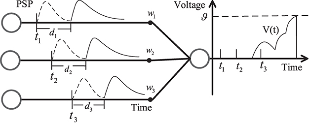
Figure 1. SRM neuron model with synaptic delay.

2.2 Learning algorithm of the SpikeProp

The SpikeProp algorithm, an improvement upon the traditional backpropagation algorithm for artificial neural networks (ANN), is designed to facilitate the learning process of multi-layer feed-forward spiking neural networks (SNN) (Bohte et al., 2002). Notably, the algorithm imposes a constraint, allowing each neuron to fire at most once within each layer. The SpikeProp algorithm employs the time minimum mean square error function as its error function, which is illustrated in Equation 4:

$\begin{array}{ll}E=\frac{1}{2}{\displaystyle \sum _k}{(t_k^o-t_k^d)}^2,& (4)\end{array}$

where $t_k^o$ represents the time at which the output neuron k emits an actual spike, and $t_k^d$ denotes its target spike time. SpikeProp utilizes the SRM model, which allows for the derivation of the relationship between firing time and membrane voltage through mathematical analysis. The weight update value is obtained by minimizing the mean square error, as defined in Equation 5:

$\begin{array}{ll}\Delta w_{ij}^l=-\eta \frac{\partial E}{\partial w_{ij}^l}=-\eta \frac{\partial E}{\partial t_j^l}\frac{\partial t_j^l}{\partial V(t_j^l)}\frac{\partial V(t_j^l)}{\partial w_{ij}^l}=-\eta ·{\delta }_j^l{K}_{ij}^l,& (5)\end{array}$

where $\Delta w_{ij}^l$ stands for the gradient of the synaptic weight between ith presynaptic neuron in layer l − 1 and jth postsynaptic neuron in layer l. ${\delta }_j^l$ is the intermediate quantity for gradient calculation, which can be expressed as $\frac{\partial E}{\partial t_j^l}\frac{\partial t_j^l}{\partial V(t_j^l)}$, and $K_{ij}^l=\frac{\partial V(t_j^l)}{\partial w_{ij}^l}=K(t_j^l-t_i^{l-1}-d_{ij}^l)$ represents the unweighted postsynaptic potential. η is the learning rate. To simplify notation, we abbreviate $V_j^l$ as V.

However, when the membrane voltage reaches the firing threshold, it promptly resets to the resting potential, resulting in a spike emission at that specific moment, rendering it non-differentiable. Consequently, the direct calculation of $\frac{\partial t_j}{\partial V(t_j^l)}$ within ${\delta }_j^l$ becomes unfeasible. To address this challenge, SpikeProp introduces the concept of a linear hypothesis. This entails assuming that within a sufficiently small neighborhood around $t=t_j^l$, the membrane potential can be reasonably approximated as a linear function of time, which is defined as:

$\begin{array}{ll}\frac{\partial t_j^l}{\partial V(t_j^l)}=\frac{-1}{\partial V(t_j^l)/\partial t}=\frac{-1}{{\displaystyle {\sum }_i}{w}_{ij}^l(\partial K_{ij}^l(t_j^l)/\partial t)}& (6)\end{array}$

2.3 The proposed learning algorithm

SpikeProp primarily focuses on adjusting synaptic weights, which is an essential aspect of biological synaptic plasticity. However, it overlooks another crucial element, synaptic delay plasticity, which imposes limitations on its overall performance and diminishes its biological interpretability. Conversely, in addressing the non-differentiability issue resulting from spike discontinuity, SpikeProp resorts to the approach outlined in Equation 6. Unfortunately, this solution introduces another challenge: the possibility of a gradient explosion due to the rapid membrane voltage change near the firing threshold. In the subsequent sections, we present solutions to these two problems individually.

2.3.1 Learning algorithms with synaptic weights and delay plasticity

To maintain generality, let's assume that the network in question is a multi-layer fully connected network, with the final layer designated as the oth layer. Similar to the approach employed in SpikeProp, the network adopts the loss function defined in Equation 4. Subsequently, based on this loss function and employing the error-backpropagation algorithm, the synaptic adjustment rules for layer l are formulated as Equation 7:

$\begin{array}{ll}\Delta d_{ij}^l(w_{ij}^l)=-{\eta }_{d(w)}\frac{\partial E}{\partial d_{ij}^l(w_{ij}^l)},& (7)\end{array}$

where $d_{ij}^l(w_{ij}^l)$ represents the synaptic delay (weight) of the connection between the ith neuron in layer l − 1 and the jth neuron in layer l. η_d(w) represents the learning rate of delays (weights). Since the adjustment of synaptic weights is the same as that of SpikeProp (i.e., Equation 5), next, we only elaborate on the learning of synaptic delay.

• Output layer: For the delay of the output layer $d_{jk}^o$, based on the chain rule, we have Equation 8:

$\begin{array}{ll}\frac{\partial E}{\partial d_{jk}^o}=\frac{\partial E}{\partial t_k^o}\frac{\partial t_k^o}{\partial V(t_k^o)}\frac{\partial V(t_k^o)}{\partial d_{jk}^o}.& (8)\end{array}$

Similarly, for the convenience of description, we define the intermediate quantity ${\delta }_k^o$ as Equation 9:

$\begin{array}{ll}{\delta }_k^o=\frac{\partial E}{\partial t_k^o}\frac{\partial t_k^o}{\partial V(t_k^o)}=\frac{\partial t_k^o}{\partial V(t_k^o)}·(t_k^o-t_k^d),& (9)\end{array}$

where $\partial t_k^o/\partial V(t_k^o)$ can be solved by Equation 6 like SpikeProp, but due to its drawbacks, we will give an alternative solution later. And the remaining terms in Equation 8 can be computed using Equation 10:

$\begin{array}{ll}\frac{\partial V(t_k^o)}{\partial d_{jk}^o}=w_{jk}^o·{\xi }_{kj}^o,& (10)\end{array}$

where

$\begin{array}{ll}\begin{array}{l}{\xi }_{kj}^o=\frac{\partial K(t_k^o-t_j^{o-1}-d_{jk}^o)}{\partial d_{jk}^o}\\ =V_{norm}\frac{1}{{\tau }_m}exp\left(-\frac{t_k^o-t_j^{o-1}-d_{jk}^o}{{\tau }_m}\right)\\ -V_{norm}\frac{1}{{\tau }_s}exp\left(-\frac{t_k^o-t_j^{o-1}-d_{jk}^o}{{\tau }_s}\right),\end{array}& (11)\end{array}$

• Hidden layer: For the delay of hidden layer $d_{ij}^l$, we have Equation 12:

$\begin{array}{ll}\frac{\partial E}{\partial d_{ij}^l}=\frac{\partial E}{\partial t_j^l}\frac{\partial t_j^l}{\partial V(t_j^l)}\frac{\partial V(t_j^l)}{\partial d_{ij}^l}={\delta }_j^l·w_{ij}^l·{\xi }_{ij}^l,& (12)\end{array}$

where $t_j^l$ is the spike time of the jth neuron in layer l. ${\delta }_j^l=\frac{\partial E}{\partial t_j^l}\frac{\partial t_j^l}{\partial V(t_j^l)}$ with

$\begin{array}{ll}\frac{\partial E}{\partial t_j^l}={\displaystyle \sum _k}\frac{\partial E}{\partial t_k^{l+1}}\frac{\partial t_k^{l+1}}{\partial V(t_k^{l+1})}\frac{\partial V(t_k^{l+1})}{\partial t_j^l}={\displaystyle \sum _k}{\delta }_k^{l+1}·w_{jk}^{l+1}{\xi }_{kj}^{l+1}.& (13)\end{array}$

To sum up, there are Equation 14:

$\begin{array}{ll}\{\begin{array}{l}\Delta w_{ij}^l=-{\eta }_w·{\delta }_j^l·K_{ij}^l,\hfill \\ \Delta d_{ij}^l=-{\eta }_d·{\delta }_j^l·w_{ij}^l{\xi }_{ij}^l,\hfill \end{array}& (14)\end{array}$

with

$\begin{array}{ll}{\delta }_j^l=\{\begin{array}{ll}\frac{\partial t_j^l}{\partial V(t_j^l)}·\left(t_j^l-t_j^d\right),\hfill & l=o\hfill \\ \frac{\partial t_j^l}{\partial V(t_j^l)}·{\displaystyle {\sum }_k{\delta }_k^{l+1}{w}_{jk}^{l+1}{\xi }_{jk}^{l+1}},\hfill & l<o\hfill \end{array}& (15)\end{array}$

While the majority of SNN algorithms traditionally focus solely on updating synaptic weights, we introduce a novel approach by incorporating the adjustment of synaptic delays. This augmentation allows us to achieve joint training of both synaptic weights and delays. This dual-training approach offers two significant advantages: addressing the silent window problem and expanding the parameter space. Silent windows, a common occurrence in spiking neural networks, refer to time periods where no spiking activity takes place, potentially undermining the learning process. Weight updates alone struggle to resolve this issue. However, incorporating delay learning can effectively adjust the distribution of input spikes and mitigate this problem. Moreover, the joint training of both synaptic weights and delays provides a more extensive set of tunable parameters compared to weight-only updates. This expanded parameter space enhances the model's flexibility and can lead to improved overall performance.

2.3.2 Gradient replacement strategy

According to the above process, it can be seen that the term $\partial t_j^l/\partial V(t_j^l)$ in Equation 15 is very important for gradient calculation. If its value is calculated according to Equation 6, it means that the derivative of the membrane voltage at the firing time will be critical. More specifically, the analysis of Figure 2A reveals that during a gradual crossing of the membrane voltage threshold, the derivative approaches zero. Consequently, this leads to a significant increase in the magnitude of $|\partial t_j^l/\partial V(t_j^l)|$, resulting in a phenomenon known as gradient explosion. To address this issue, we draw upon the insights from the rectangle replacement function (Wu et al., 2018), which has demonstrated enhanced convergence in ablation experiments. Building upon this framework, we propose a novel replacement function that mitigates the problem of gradient explosion. As a result, Equation 6 can be replaced by Equation 16, as shown below.

$\begin{array}{ll}\frac{\partial t_j^l}{\partial V(t_j^l)}=\{\begin{array}{ll}\exp \left(-\frac{2{\left(V(t_j^l)-\vartheta \right)}^2}{\tau }\right),\hfill & |V(t_j^l)-\vartheta |>m,\hfill \\ \exp \left(-\frac{2m^2}{\tau }\right),\hfill & |V(t_j^l)-\vartheta |\le m.\hfill \end{array}& (16)\end{array}$

where m (0 < m < 1) is a constant, and there is currently no accepted theoretical method for finding the optimal m on any dataset. But a good way to get an appropriate m for a specific task is to use parameter search.

Figure 2

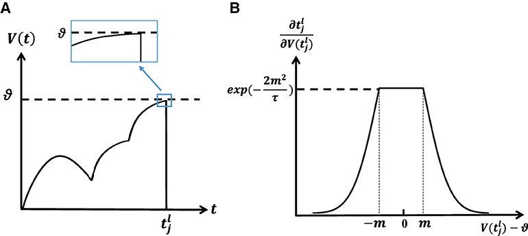
Figure 2. (A) Membrane potential reaches the threshold slowly, resulting in the exploding gradient. (B) The shape of the surrogate gradient function.

Figure 2B shows the shape of replaced weight. The closer the membrane potential is to the firing time than to the threshold, the larger $\partial t_j^l/\partial V(t_j^l)$, which is consistent with the characteristics of the spike activity. However, it's important to emphasize that this value cannot become infinitely large since it would cause the value of Equation 6 to approach 0, leading the gradient to disappear. In our approach, we impose an upper limit, capping it at exp(−2m²/τ). This constraint ensures that the influence on $\partial t_j^l/\partial V(t_j^l)$ remains bounded. Actually, the function of the surrogate gradient can be various (Wu et al., 2018).

3 Results

In this section, we test the performance of the proposed algorithm on several different datasets, including Iris, Breast Cancer, Liver Disorders, Pima Diabetes, and Ionosphere. By comparison with other algorithms: SpikeProp (Shrestha and Song, 2015), SpikeTemp (Wang et al., 2015), SWAT (Wade et al., 2010), ReSuMe (Ponulak and Kasiński, 2010), SRESN (Dora et al., 2016), and MDL (Taherkhani et al., 2018), the proposed method has a good performance.

The datasets can be divided into two types: real-value datasets and image-related datasets. Samples from these databases cannot be fed directly into the network and need to be encoded into spike sequences. In real-value datasets, the population encoding (Bohte et al., 2002; Shrestha and Song, 2015; Wang et al., 2015; Taherkhani et al., 2018) is used to convert these values to input spike trains, as shown in Figure 3. In image datasets, the latency encoding (Hopfield, 1995; Hu et al., 2013) is used, as shown in Figure 4.

Figure 3

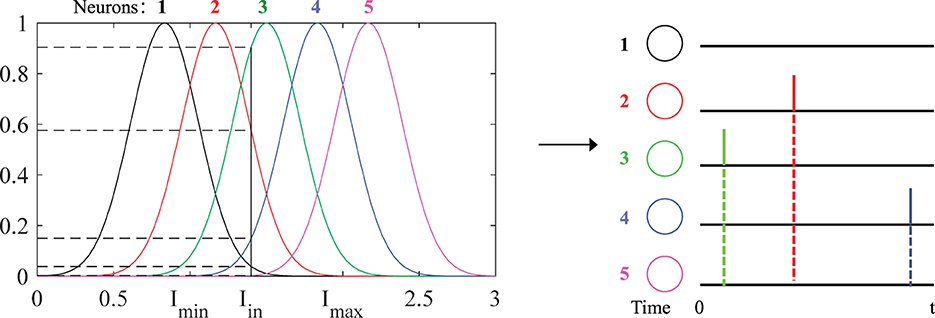
Figure 3. Schematic diagram of population encoding. Each neuron has its own Gaussian receiving function (different colors). I_min and I_max are the minimum and maximum values of the input current. When an input current I_in is fed, the corresponding value on the Gaussian function is its probability value. Finally, these values are encoded into the spiking times distributed in [0, t]. The larger probability value corresponds to the earlier spiking time and vice versa, and the spikes will not be emitted if the firing threshold is not reached, such as neurons “1” and “5.”

Figure 4

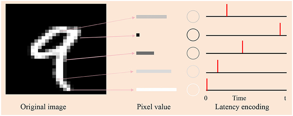
Figure 4. Schematic diagram of latency encoding. The subfigure on the left is an original image of the digit “9” in the MNIST. Its pixel values determine the brightness of each pixel, with higher values corresponding to whiter areas. Depending on the value, we draw five rectangles (in the middle subfigure) of different widths to represent different pixel values, with wider rectangles representing larger values. The right subfigure is the spiking times of the selected five neurons by latency encoding. The larger the pixel value, the earlier the firing time.

In the output layer each output neuron corresponds to a category, and when a training sample is fed, the corresponding output neuron is trained to fire at desired output spike time t_d generated by the dynamic decoding method (Luo et al., 2019; Zhang Y. et al., 2021), while the other neurons are kept silent.

3.1 Classification of Iris dataset

As one of the most well-known pattern recognition databases, it is divided into three categories. Each category has 50 samples with four attributes: sepal length, sepal width, petal length, and petal width. Among them, 25 samples of each category were used as the training set, and the others were used as the test set. The network structure is 25-20-3, and a sample is considered correctly classified if either its target neuron fire the most spikes or the membrane potential of its target neuron is the maximum when none of the output neurons fire. The network architecture, training epochs, train and test accuracy of our works and the contrasting methods are all depicted in Table 1. The contrast of train and test accuracy of all methods are further illustrated in Figure 5. From the results, the proposed method outperforms these methods: SpikeProp, SWAT, MDL, ReSuMe, and SpikeTemp. SRESN achieved the best test accuracy, and the proposed model is only slightly below it.

Table 1

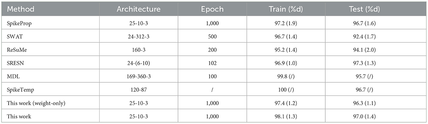
Table 1. Classification results of Iris database.

Figure 5

Figure 5. The training accuracy and test accuracy for various methods on Iris database. The best training accuracy of all methods is SpikeTemp, but the best test accuracy is SRESN which is 0.3% higher than the proposed algorithm.

3.2 Classification of Breast Cancer dataset

The data were collected from clinical studies conducted between January 2014 and December 2014 and were derived from microscopic biopsy images of breast lumps in patients with breast cancer. Each sample has 10 attributes to describe the characteristics of the nucleus of the mass, including radius, texture, perimeter, and so on. It is divided into two types of data: benign and malignant cancers. This dataset has 569 instances, of which 357 are benign and the remaining 212 are malignant. Among them, 179 benign samples and 106 malignant samples make up the training set, and the rest were used as test sets. The network architecture of the proposed method is 55-15-2. Two output neurons correspond to the benign sample and the malignant sample. If the benign output neuron fires the more spikes or has a larger membrane potential than the malignant one, the benign sample was correctly classified; and vice versa. The network architecture, training epochs, train and test accuracy of our works are shown in Table 2, along with those of the other methods. Additionally, the contrast of train and test accuracy of all methods are further illustrated in Figure 6. Experimental results show that this method outperforms most comparison algorithms including SpikeProp, SWAT, ReSuMe, SRESN, and MDL. And our model is only 0.4% lower than SpikeTemp.

Table 2

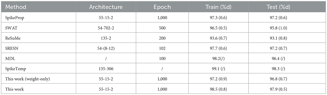
Table 2. Classification results of Breast Cancer database.

Figure 6

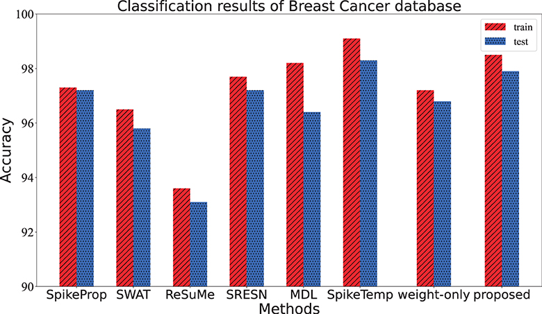
Figure 6. The training accuracy and test accuracy for various methods on Breast Cancer database. The training and test accuracy of the proposed method is the second, slightly lower than SpikeTemp.

3.3 Classification of Liver Disorders dataset

This dataset consisted of 345 samples of seven attributes, amongst which the first five attributes are blood data related to the development of liver disease, and the sixth attribute is the number of alcoholic drinks per day. It is a binary classification, with half of the data in each category comprising the training set and the other half comprising the test set. The input neurons, hidden neurons and output neurons are 37, 15, and 2, respectively. If the target neuron of a sample fires the overwhelming spikes or has the larger membrane potential, this sample is considered to be correctly classified. The performance of the proposed method in Table 3 and Figure 7 comes from the average of 20 trials with 3,000 training epochs, which outperforms other methods in terms of test accuracy.

Table 3

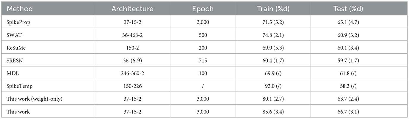
Table 3. Classification results of Liver Disorders database.

Figure 7

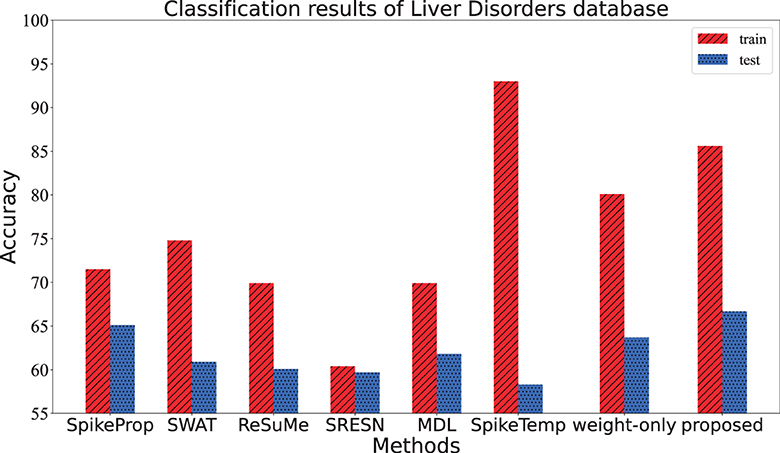
Figure 7. The training accuracy and test accuracy for various methods on Liver Disorders database. The training accuracy of the SpikeTemp is the best, while the test accuracy of the proposed method is the best.

3.4 Classification of Pima Diabetes dataset

This dataset contains women of at least 21 years of Pima Indian ancestry. It is also a binary classification to predict whether a patient has diabetes or not on the basis of eight attributes, including Pregnancy, Glucose, Glucose, etc. The data set includes 768 samples that are divided into training/test sets in a 1:1 ratio. The network structure is 55-20-2, and the conditions for correct classification are as follows: (1) the target output neuron of the input sample fires the most spikes, (2) the membrane potential of the target neuron overwhelms the other one when firing the same spikes. After 20 training trials of 3,000 epochs, the accuracy of our model is shown in Table 4. From Table 4 and Figure 8, the training and test accuracy of the proposed method are much higher than the all the other contrasting methods.

Table 4

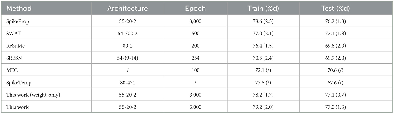
Table 4. Classification results of Pima Diabetes database.

Figure 8

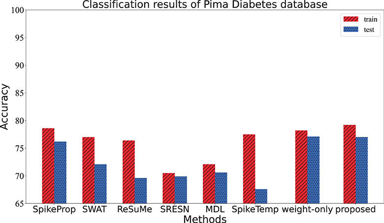
Figure 8. The training accuracy and test accuracy for various methods on Pima Diabetes database. The training accuracy and test accuracy of the proposed method is the best.

3.5 Classification of Ionosphere dataset

This dataset contains 351 samples of radar data collected by Johns Hopkins University. Each sample consists of 35 attributes, the first 34 attributes are contiguous, and the last attribute is the category label. This data set has two categories, and equal numbers of the samples from each category were added to the training set and test set respectively. The network architecture of this experiment is 205-25-2. When a sample is fed into the network, the category is determined if its target neuron emits the most spikes, or if the target neuron has the maximum membrane potential when emitting the same number of spikes as the other neuron. The network is trained 3,000 epochs in each trial, and the average of 20 trials is shown in Table 5. From Table 5 and Figure 9, the test accuracy of the proposed model ranks only below spikeTemp with a slight gap, but obviously higher than the other five comparison algorithms.

Table 5

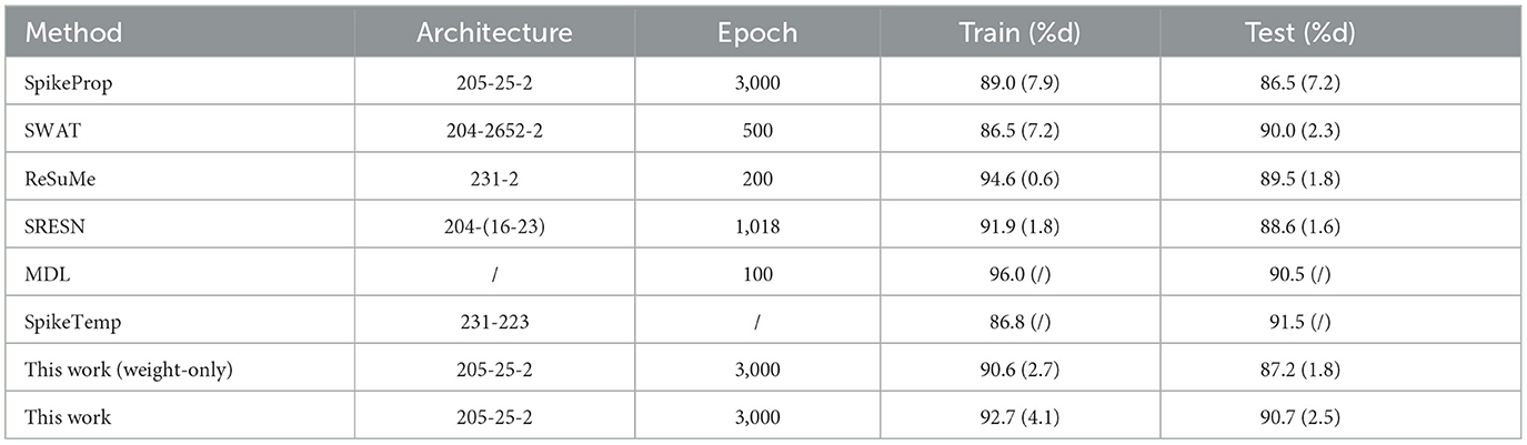
Table 5. Classification results of Ionosphere database.

Figure 9

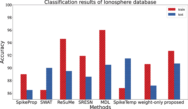
Figure 9. The training accuracy and test accuracy for various methods on Ionosphere database. The proposed method gets the best test accuracy and the smallest gap between training accuracy and test accuracy.

3.6 Classification of MNIST dataset

To exploit and testify the image information learning capacity of the proposed method, we conducted experiments on the widely used MNIST dataset (LeCun et al., 1998), which is a popular choice in deep learning research (Mostafa, 2017; Tavanaei and Maida, 2019; Comsa et al., 2020). This dataset comprises 60,000 training samples and 10,000 testing samples, each of which has a visual scale of 28 × 28 pixels. The pixels are encoded as spike trains through the latency encoding method (Hopfield, 1995) and then fed in the proposed method with the architecture 784-800-10. We compare the experimental results with some effective ANN and SNN works, as detailed in Table 6. The results show that the proposed model has a comparable performance on image data, which outperforms the contrasting SNN models, and only trivially falls behind artificial neural networks in terms of accuracy.

Table 6

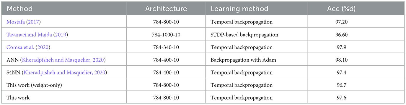
Table 6. Comparison with other works on MNIST dataset.

4 Discussion

In this paper, we proposed a new supervised learning algorithm for multi-layer spiking neural networks, which considers the plasticity of both synaptic weights and delays. Various experiments are conducted to verify the performance of the proposed learning method, and the experimental results support its superiority. Actually, how to train multilayer spiking neural networks remains an open question. The existing learning rules can be classified as ANN-to-SNN, surrogate gradient method, and spike-driven learning algorithms. In the following, we will compare the proposed method with these methods.

4.1 Compared to ANN-to-SNN methods

The ANN-to-SNN methods are proposed to avoid the difficult training of deep spiking neural networks. However, most of the ANN-to-SNN methods are based on the spike rate information, the time information has not been fully leveraged. In addition, the existing ANN-to-SNN conversion methods can only deal with image datasets. Those datasets with rich temporal information like speech and video can not be addressed by these methods. Our algorithm adopts temporal coding to make full use of the time information of spikes and has more potential to process these temporal datasets.

4.2 Compared to surrogate gradient methods

Due to the non-differentiable spike function, directly training spiking neural networks is very difficult. To resolve this problem, surrogate gradient-based learning algorithms are proposed. By using a surrogate gradient, these methods do not need to calculate the exact gradients. However, these methods need to do backpropagation at every time step and cost a lot of computing sources. In contrast, our algorithm holds the potential of enabling training and inference in low-power devices.

4.3 Compared to spike-driven methods

There are various spike-driven learning methods, such as SpikeProp and STDBP. However, most existing spike-driven learning algorithms only consider the plasticity of synaptic weights and ignore synaptic delay adjustment. In our algorithm, both the synaptic weights and delays are considered adjustable variables to improve both the biological plausibility and the learning performance. Experimental results demonstrate that our algorithm achieves a competitive learning performance compared with the existing related works. In the future, we would like to further extend the application of spike-driven learning algorithms on large-scale datasets and other practical applications (Liu and Li, 2022; Liu et al., 2022a,b).

Data availability statement

The original contributions presented in the study are included in the article/supplementary material, further inquiries can be directed to the corresponding author.

Author contributions

JW: Conceptualization, Methodology, Writing – original draft, Writing – review & editing.

Funding

This work was supported by the National Science Foundation of China under Grant 61976043.

Conflict of interest

The author declares that the research was conducted in the absence of any commercial or financial relationships that could be construed as a potential conflict of interest.

Publisher's note

All claims expressed in this article are solely those of the authors and do not necessarily represent those of their affiliated organizations, or those of the publisher, the editors and the reviewers. Any product that may be evaluated in this article, or claim that may be made by its manufacturer, is not guaranteed or endorsed by the publisher.

References

Arulkumaran, K., Deisenroth, M. P., Brundage, M., and Bharath, A. A. (2017). Deep reinforcement learning: a brief survey. IEEE Signal Process. Mag. 34, 26–38. doi: 10.1109/MSP.2017.2743240

Crossref Full Text | Google Scholar

Bohte, S. M., Kok, J. N., and La Poutre, H. (2002). Error-backpropagation in temporally encoded networks of spiking neurons. Neurocomputing 48, 17–37. doi: 10.1016/S0925-2312(01)00658-0

Crossref Full Text | Google Scholar

Caporale, N., and Dan, Y. (2008). Spike timing-dependent plasticity: a Hebbian learning rule. Annu. Rev. Neurosci. 31, 25–46. doi: 10.1146/annurev.neuro.31.060407.125639

PubMed Abstract | Crossref Full Text | Google Scholar

Comsa, I. M., Potempa, K., Versari, L., Fischbacher, T., Gesmundo, A., Alakuijala, J., et al. (2020). “Temporal coding in spiking neural networks with alpha synaptic function,” in ICASSP 2020-2020 IEEE International Conference on Acoustics, Speech and Signal Processing (ICASSP) (Barcelona: IEEE), 8529–8533. doi: 10.1109/ICASSP40776.2020.9053856

PubMed Abstract | Crossref Full Text | Google Scholar

Dora, S., Subramanian, K., Suresh, S., and Sundararajan, N. (2016). Development of a self-regulating evolving spiking neural network for classification problem. Neurocomputing 171, 1216–1229. doi: 10.1016/j.neucom.2015.07.086

Crossref Full Text | Google Scholar

Gerstner, W. (1995). Time structure of the activity in neural network models. Phys. Rev. E 51, 738. doi: 10.1103/PhysRevE.51.738

PubMed Abstract | Crossref Full Text | Google Scholar

Ghosh-Dastidar, S., and Adeli, H. (2009). Spiking neural networks. Int. J. Neural Syst. 19, 295–308. doi: 10.1142/S0129065709002002

Crossref Full Text | Google Scholar

Gütig, R. (2016). Spiking neurons can discover predictive features by aggregate-label learning. Science 351, aab4113. doi: 10.1126/science.aab4113

PubMed Abstract | Crossref Full Text | Google Scholar

Han, Y., Xiang, S., Ren, Z., Fu, C., Wen, A., Hao, Y., et al. (2021). Delay-weight plasticity-based supervised learning in optical spiking neural networks. Photonics Res. 9, 119–127. doi: 10.1364/PRJ.413742

Crossref Full Text | Google Scholar

He, K., Zhang, X., Ren, S., and Sun, J. (2016). “Deep residual learning for image recognition,” in 2016 IEEE Conference on Computer Vision and Pattern Recognition (CVPR) (Las Vegas, NV: IEEE), 770–778. doi: 10.1109/CVPR.2016.90

Crossref Full Text | Google Scholar

Hopfield, J. J. (1995). Pattern recognition computation using action potential timing for stimulus representation. Nature 376, 33–36. doi: 10.1038/376033a0

PubMed Abstract | Crossref Full Text | Google Scholar

Hu, J., Tang, H., Tan, K. C., Li, H., and Shi, L. (2013). A spike-timing-based integrated model for pattern recognition. Neural Comput. 25, 450–472. doi: 10.1162/NECO_a_00395

PubMed Abstract | Crossref Full Text | Google Scholar

Izhikevich, E. M. (2003). Simple model of spiking neurons. IEEE Trans. Neural Netw. 14, 1569–1572. doi: 10.1109/TNN.2003.820440

PubMed Abstract | Crossref Full Text | Google Scholar

Kheradpisheh, S. R., and Masquelier, T. (2020). Temporal backpropagation for spiking neural networks with one spike per neuron. Int. J. Neural Syst. 30, 2050027. doi: 10.1142/S0129065720500276

PubMed Abstract | Crossref Full Text | Google Scholar

Lan, Y., Wang, X., and Wang, Y. (2021). Spatio-temporal sequential memory model with mini-column neural network. Front. Neurosci. 15, 374. doi: 10.3389/fnins.2021.650430

PubMed Abstract | Crossref Full Text | Google Scholar

LeCun, Y., Bottou, L., Bengio, Y., and Haffner, P. (1998). Gradient-based learning applied to document recognition. Proc. IEEE 86, 2278–2324. doi: 10.1109/5.726791

Crossref Full Text | Google Scholar

Liu, Q., and Li, X. (2022). Efficient low-rank matrix factorization based on ℓ1,ε-norm for online background subtraction. IEEE Trans. Circuits Syst. Video Technol. 32, 4900–4904. doi: 10.1109/TCSVT.2021.3129503

Crossref Full Text | Google Scholar

Liu, Q., Li, X., Cao, H., and Wu, Y. (2022a). From simulated to visual data: a robust low-rank tensor completion approach using ℓp-regression for outlier resistance. IEEE Trans. Circuits Syst. Video Technol. 32, 3462–3474. doi: 10.1109/TCSVT.2021.3114208

Crossref Full Text | Google Scholar

Liu, Q., Li, X., and Yang, J. (2022b). Optimum codesign for image denoising between type-2 fuzzy identifier and matrix completion denoiser. IEEE Trans. Fuzzy Syst. 30, 287–292. doi: 10.1109/TFUZZ.2020.3030498

Crossref Full Text | Google Scholar

Luo, X., Qu, H., Wang, Y., Yi, Z., Zhang, J., Zhang, M., et al. (2022). Supervised learning in multilayer spiking neural networks with spike temporal error backpropagation. IEEE Trans. Neural Netw. Learn. Syst. 34, 10141–10153. doi: 10.1109/TNNLS.2022.3164930

PubMed Abstract | Crossref Full Text | Google Scholar

Luo, X., Qu, H., Zhang, Y., and Chen, Y. (2019). First error-based supervised learning algorithm for spiking neural networks. Front. Neurosci. 13, 559. doi: 10.3389/fnins.2019.00559

PubMed Abstract | Crossref Full Text | Google Scholar

Maass, W. (1997). Networks of spiking neurons: the third generation of neural network models. Neural Netw. 10, 1659–1671. doi: 10.1016/S0893-6080(97)00011-7

Crossref Full Text | Google Scholar

Maass, W., and Bishop, C. M. (2001). Pulsed Neural Networks. Cambridge, MA: MIT press.

Google Scholar

Mostafa, H. (2017). Supervised learning based on temporal coding in spiking neural networks. IEEE Trans. Neural Netw. Learn. Syst. 29, 3227–3235. doi: 10.1109/TNNLS.2017.2726060

PubMed Abstract | Crossref Full Text | Google Scholar

Neftci, E. O., Charles, A., Somnath, P., and Georgios, D. (2016). Event-driven random back-propagation: enabling neuromorphic deep learning machines. Front. Neurosci. 11, 324. doi: 10.3389/fnins.2017.00324

PubMed Abstract | Crossref Full Text | Google Scholar

Neftci, E. O., Mostafa, H., and Zenke, F. (2019). Surrogate gradient learning in spiking neural networks: bringing the power of gradient-based optimization to spiking neural networks. IEEE Signal Process. Mag. 36, 51–63. doi: 10.1109/MSP.2019.2931595

Crossref Full Text | Google Scholar

Pan, Z., Zhang, M., Wu, J., Wang, J., and Li, H. (2021). Multi-tone phase coding of interaural time difference for sound source localization with spiking neural networks. IEEE/ACM Trans. Audio Speech Lang. Process. 29, 2656–2670. doi: 10.1109/TASLP.2021.3100684

Crossref Full Text | Google Scholar

Pfeiffer, M., and Pfeil, T. (2018). Deep learning with spiking neurons: opportunities and challenges. Front. Neurosci. 12, 774. doi: 10.3389/fnins.2018.00774

PubMed Abstract | Crossref Full Text | Google Scholar

Ponulak, F., and Kasiński, A. (2010). Supervised learning in spiking neural networks with resume: sequence learning, classification, and spike shifting. Neural Comput. 22, 467–510. doi: 10.1162/neco.2009.11-08-901

PubMed Abstract | Crossref Full Text | Google Scholar

Shrestha, S., and Orchard, G. (2018). “Slayer: spike layer error reassignment in time,” in Advances in Neural Information Processing Systems, Vol. 31, 1419–1428.

Google Scholar

Shrestha, S. B., and Song, Q. (2015). Adaptive learning rate of spikeprop based on weight convergence analysis. Neural Netw. 63, 185–198. doi: 10.1016/j.neunet.2014.12.001

PubMed Abstract | Crossref Full Text | Google Scholar

Subakan, C., Ravanelli, M., Cornell, S., Bronzi, M., and Zhong, J. (2021). “Attention is all you need in speech separation,” in ICASSP 2021 - 2021 IEEE International Conference on Acoustics, Speech and Signal Processing (ICASSP) (Toronto, ON: IEEE), 21–25. doi: 10.1109/ICASSP39728.2021.9413901

Crossref Full Text | Google Scholar

Sun, P., Eqlimi, E., Chua, Y., Devos, P., and Botteldooren, D. (2023). “Adaptive axonal delays in feedforward spiking neural networks for accurate spoken word recognition,” in ICASSP 2023-2023 IEEE International Conference on Acoustics, Speech and Signal Processing (ICASSP) (Rhodes Island: IEEE), 1–5. doi: 10.1109/ICASSP49357.2023.10094768

Crossref Full Text | Google Scholar

Sun, P., Zhu, L., and Botteldooren, D. (2022). “Axonal delay as a short-term memory for feed forward deep spiking neural networks,” in ICASSP 2022-2022 IEEE International Conference on Acoustics, Speech and Signal Processing (ICASSP) (Singapore: IEEE), 8932–8936. doi: 10.1109/ICASSP43922.2022.9747411

Crossref Full Text | Google Scholar

Taherkhani, A., Belatreche, A., Li, Y., and Maguire, L. P. (2015a). Dl-resume: a delay learning-based remote supervised method for spiking neurons. IEEE Trans. Neural Netw. Learn. Syst. 26, 3137–3149. doi: 10.1109/TNNLS.2015.2404938

PubMed Abstract | Crossref Full Text | Google Scholar

Taherkhani, A., Belatreche, A., Li, Y., and Maguire, L. P. (2015b). “Multi-dl-resume: multiple neurons delay learning remote supervised method,” in 2015 International Joint Conference on Neural Networks (IJCNN) (Killarney: IEEE), 1–7. doi: 10.1109/IJCNN.2015.7280743

Crossref Full Text | Google Scholar

Taherkhani, A., Belatreche, A., Li, Y., and Maguire, L. P. (2018). A supervised learning algorithm for learning precise timing of multiple spikes in multilayer spiking neural networks. IEEE Trans. Neural Netw. Learn. Syst. 29, 5394–5407. doi: 10.1109/TNNLS.2018.2797801

PubMed Abstract | Crossref Full Text | Google Scholar

Tavanaei, A., and Maida, A. (2019). Bp-stdp: approximating backpropagation using spike timing dependent plasticity. Neurocomputing 330, 39–47. doi: 10.1016/j.neucom.2018.11.014

Crossref Full Text | Google Scholar

Wade, J. J., McDaid, L. J., Santos, J. A., and Sayers, H. M. (2010). Swat: a spiking neural network training algorithm for classification problems. IEEE Trans. Neural Netw. 21, 1817–1830. doi: 10.1109/TNN.2010.2074212

PubMed Abstract | Crossref Full Text | Google Scholar

Wang, J., Belatreche, A., Maguire, L. P., and McGinnity, T. M. (2015). Spiketemp: an enhanced rank-order-based learning approach for spiking neural networks with adaptive structure. IEEE Trans. Neural Netw. Learn. Syst. 28, 30–43. doi: 10.1109/TNNLS.2015.2501322

PubMed Abstract | Crossref Full Text | Google Scholar

Wu, J., Chua, Y., Zhang, M., Li, G., Li, H., Tan, K. C., et al. (2021a). A tandem learning rule for effective training and rapid inference of deep spiking neural networks. IEEE Trans. Neural Netw. Learn. Syst. 34, 446–460. doi: 10.1109/TNNLS.2021.3095724

PubMed Abstract | Crossref Full Text | Google Scholar

Wu, J., Xu, C., Han, X., Zhou, D., Zhang, M., Li, H., et al. (2021b). Progressive tandem learning for pattern recognition with deep spiking neural networks. IEEE Trans. Pattern Anal. Mach. Intell. 44, 7824–7840. doi: 10.1109/TPAMI.2021.3114196

PubMed Abstract | Crossref Full Text | Google Scholar

Wu, J., Zhan, Y., Peng, Z., Ji, X., and Wang, C. (2021c). Efficient design of spiking neural network with stdp learning based on fast cordic. IEEE Trans. Circuits Syst. I: Regul. Pap. 68, 2522–2534. doi: 10.1109/TCSI.2021.3061766

Crossref Full Text | Google Scholar

Wu, Y., Deng, L., Li, G., Zhu, J., and Shi, L. (2018). Spatio-temporal backpropagation for training high-performance spiking neural networks. Front. Neurosci. 12, 331. doi: 10.3389/fnins.2018.00331

PubMed Abstract | Crossref Full Text | Google Scholar

Yha, B., Xh, A., Meng, D. A., and Bo, X. (2020). A biologically plausible supervised learning method for spiking neural networks using the symmetric stdp rule. Neural Netw. 121, 387–395. doi: 10.1016/j.neunet.2019.09.007

PubMed Abstract | Crossref Full Text | Google Scholar

Zhang, M., Wang, J., Wu, J., Belatreche, A., Amornpaisannon, B., Zhang, Z., et al. (2021). Rectified linear postsynaptic potential function for backpropagation in deep spiking neural networks. IEEE Trans. Neural Netw. Learn. Syst. 33, 1947–1958. doi: 10.1109/TNNLS.2021.3110991

PubMed Abstract | Crossref Full Text | Google Scholar

Zhang, M., Wu, J., Belatreche, A., Pan, Z., Xie, X., Chua, Y., et al. (2020). Supervised learning in spiking neural networks with synaptic delay-weight plasticity. Neurocomputing 409, 103–118. doi: 10.1016/j.neucom.2020.03.079

Crossref Full Text | Google Scholar

Zhang, Y., Chen, Y., Zhang, J., Luo, X., Zhang, M., Qu, H., et al. (2022). Minicolumn-based episodic memory model with spiking neurons, dendrites and delays. IEEE Trans. Neural Netw. Learn. Syst. 1–15. doi: 10.1109/TNNLS.2022.3213688

PubMed Abstract | Crossref Full Text | Google Scholar

Zhang, Y., Qu, H., Luo, X., Chen, Y., Wang, Y., Zhang, M., et al. (2021). A new recursive least squares-based learning algorithm for spiking neurons. Neural Netw. 138, 110–125. doi: 10.1016/j.neunet.2021.01.016

PubMed Abstract | Crossref Full Text | Google Scholar

Zhu, X., Zhao, B., Ma, D., and Tang, H. (2021). An efficient learning algorithm for direct training deep spiking neural networks. IEEE Trans. Cogn. Develop. Syst. 14, 847–856. doi: 10.1109/TCDS.2021.3073846

Crossref Full Text | Google Scholar