Simulating Longitudinal Brain MRIs with Known Volume Changes and Realistic Variations in Image Intensity

This paper presents a simulator tool that can simulate large databases of visually realistic longitudinal MRIs with known volume changes. The simulator is based on a previously proposed biophysical model of brain deformation due to atrophy in AD. In this work, we propose a novel way of reproducing realistic intensity variation in longitudinal brain MRIs, which is inspired by an approach used for the generation of synthetic cardiac sequence images. This approach combines a deformation field obtained from the biophysical model with a deformation field obtained by a non-rigid registration of two images. The combined deformation field is then used to simulate a new image with specified atrophy from the first image, but with the intensity characteristics of the second image. This allows to generate the realistic variations present in real longitudinal time-series of images, such as the independence of noise between two acquisitions and the potential presence of variable acquisition artifacts. Various options available in the simulator software are briefly explained in this paper. In addition, the software is released as an open-source repository. The availability of the software allows researchers to produce tailored databases of images with ground truth volume changes; we believe this will help developing more robust brain morphometry tools. Additionally, we believe that the scientific community can also use the software to further experiment with the proposed model, and add more complex models of brain deformation and atrophy generation.

1. Introduction

Structural Magnetic Resonance Imaging (MRI) has been widely used for in vivo observation of morphological changes over time in human brain. Atrophy or tissue volume loss measure from structural MRI is an established biomarker for neurodegeneration (Frisoni et al., 2010). There is a large number of brain morphometry algorithms developed in the literature which estimate global or local atrophy from structural MRIs (Wright et al., 1995; Freeborough and Fox, 1997; Ashburner and Friston, 2000; Smith et al., 2002; Hua et al., 2008). Volume/atrophy measurements obtained from such algorithms have been used to test various clinical hypotheses about neurodegenerative diseases (Wright et al., 1995; Sepulcre et al., 2006; Koch et al., 2016). Similarly, comparison of different neurodegenerative diseases have also been performed based on these measurements (Rosen et al., 2002; Whitwell and Jack, 2005). Since atrophy estimation is an inverse problem, the estimation algorithms require a model with certain parameters. The results obtained from such algorithms depend on model assumptions and the parameters used. Often, these assumptions are implicit and cannot be directly linked to the biophysical process of neurodegeneration. For instance, tensor based morphometry (TBM) encodes local volume changes by computing Jacobian determinants of the deformation field obtained from non-linear registration of longitudinal MRIs (Ashburner and Ridgway, 2015). Such methods contain model biases because TBM results depend on the choices of regularization used during the registration of images (Ashburner, 2013). Likewise, edge-based methods such as BSI, SIENA etc. are sensitive to unmatched image contrasts between scans, poor signal-to-noise ratio, partial volume effects, segmentation errors etc. (Preboske et al., 2006; Prados et al., 2015). Estimating and correcting the bias present in such morphometry tools is important, especially for clinical applications.

In addition to tracking volumetric changes in specific brain structures, longitudinal imaging data can also be used to study the temporal inter-relationship of atrophy in different structures. For instance, Carmichael et al. (2013) studied the groupings of 34 cortical regions and hippocampi from the per-individual rates of atrophy estimates in these regions. In Fonteijn et al. (2012), authors defined AD progression as a series of discrete events. Along with other clinical events, the timings of atrophy in various brain structures were included in a set of discrete events. Without any prior to their ordering, the model finds the most probable order for these events from the data itself. They used Bayesian statistical algorithms for fitting the event-based disease progression model. The objective of these studies were to understand how different regions of brain evolve during the neurodegeneration.

In this context of increasing use of the atrophy measurements from longitudinal MRIs in testing or discovering clinically relevant hypotheses, it is important to study the bias and variability of the atrophy estimation algorithms. The actual volume changes in real longitudinal MRIs are not known. Thus, the evaluation and validation of atrophy estimation algorithms require generating images with known volume changes, called ground truth images.

A number of atrophy simulators have been proposed in the literature to produce ground truth MRIs (Smith et al., 2003; Camara et al., 2006; Karaçali and Davatzikos, 2006; Pieperhoff et al., 2008; Sharma et al., 2010; Modat et al., 2014; Radua et al., 2014; Khanal et al., 2016a). Most of these simulators use a model that attempts to produce a deformation field with the specified volume changes in the input brain MRI. To produce realistic scenarios of noise and acquisition artifacts, some of these simulators also use a model to produce noise and artifacts in the simulated image.

Such simulators have been used for the validation of registration or segmentation based atrophy estimation algorithms (Camara et al., 2008; Pieperhoff et al., 2008; Sharma et al., 2010), to estimate the bias in such algorithms, and also to estimate uncertainty in the measured atrophy (Sharma et al., 2013). These studies have estimated the bias by simulating simple atrophy patterns in a small number of brain regions or uniform diffused global atrophies. However, real case scenarios could have a much more complex atrophy distribution occurring in many brain structures at the same time.

Noise and imaging artifacts have an important impact on the results obtained from atrophy estimation algorithms (Camara et al., 2008; Pieperhoff et al., 2008; Sharma et al., 2010). Thus, proper evaluation of atrophy estimation algorithms by using simulated ground truth images requires simulation of realistic variation in noise and intensity too. All the previous atrophy simulators have warped the input baseline image with the deformation field obtained from a model of brain deformation. Then, extra noise and artifacts are added on this warped image by using another artificial model. The intensity noise in structural MRIs has been shown to be governed by a Rician distribution where the noise is Gaussian in k-space (Gudbjartsson and Patz, 1995). Thus, the Rician noise can be added in the simulated images as follows:

• Use two independent random variables following zero-mean Gaussian distribution to compute the real and imaginary parts of a complex number at each voxel.

• Considering the original intensity to be a complex number with zero imaginary part, add the real and imaginary components obtained above and take the magnitude of the resulting complex signal.

For example, Sled et al. (1998) used this approach to add noise in simulated MRIs that were used for the validation of intensity bias correction scheme they presented. Using the same approach, Camara et al. (2008) added noise to the simulated ground truth images with atrophy.

In addition to the Rician noise described above, other noise, and artifacts are also present in MRIs (Simmons et al., 1994). Some of the artifact sources that have been shown to affect the measurements of atrophy estimation algorithms (Camara-Rey et al., 2006; Pieperhoff et al., 2008; Sharma et al., 2010) are:

• Bias field inhomogeneity arising due to poor radio frequency (RF) coil uniformity.

• Geometrical distortions that are present due to the errors in gradient field strength and non-linearity of gradient fields in the MR scanner (Langlois et al., 1999).

• Interpolation of intensities during various pre-processing steps of TBM based analysis framework (e.g., resampling of the images into a common template space).

Many other acquisition artifacts may not be simulated because we do not have faithful models. Inability to produce realistic intensity variation and noise in simulated longitudinal images is one of the key limitations in the state-of-the-art atrophy simulators, including our previous work (Khanal et al., 2016a). In this work, we propose a simple but elegant solution to remove the limitation of previous atrophy simulators. First, our biophysical model of brain deformation (Khanal et al., 2016a) is used to obtain a dense deformation field with specified volume changes. Then, to obtain realistic intensity variations, intensities in the simulated images are resampled from baseline repeat scans of the same patient. Although the method is very simple and straightforward, this allows simulating longitudinal images with variation in intensity and noise taken from real scans themselves without explicitly specifying any noise or artifact models. To the best of our knowledge, this idea was not presented before in the literature. When the repeat scans are not available, we use an approach introduced by Prakosa et al. (2013) where the authors simulate visually realistic time series of cardiac images. Intensity variation in the simulated images of a patient is obtained by resampling the intensities from the repeat scans if available, otherwise from the real images of the same patient taken at different times.

Figure 1 shows a diagram of the complete framework. To implement this framework, we have developed an open-source atrophy simulator software called Simul@trophy¹. To our knowledge, Simul@trophy is the first atrophy simulator to be made open-source. Simul@trophy uses the biophysical model presented in Khanal et al. (2016a) but introduces a new numerical scheme to compute divergence, which removes the numerical inconsistency presented in the previous work. This is further explained in detail in Section 4.2.

FIGURE 1

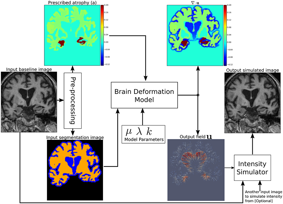
Figure 1. Pipeline to simulate synthetic images using Simul@trophy. Starting from a real baseline image of a subject, synthetic images with known volume changes can be generated. These synthetic images can follow intensity characteristics of either the input baseline or other images of the same subject. Pre-processing is required to generate an atrophy map and a segmentation image, which are fed as inputs to the brain deformation model. For a given set of parameters, the model computes a velocity field whose divergence is equal to the prescribed atrophy map at each voxel of the regions selected by using the segmentation image. Intensity simulator uses the output field to produce synthetic image whose intensity is resampled either from the input real baseline or from any other image as desired.

Section 2 explains all the blocks of the framework shown in Figure 1. Starting from a small set of real scans, we show how longitudinal images with different atrophy patterns and realistic intensity variations can be simulated. Section 3 shows some simulation results using Simul@trophy, and also illustrates some potential applications of the simulator. In Section 4, we present some example simulations to illustrate some of the important points to consider when using Simul@trophy for different applications, such as evaluation of atrophy estimation algorithms, validation of data-driven disease progression models, training of brain morphometry algorithms based on machine learning etc.

2. Simulating Realistic Longitudinal Images with Atrophy/Growth

We use the biophysical model presented in Khanal et al. (2014, 2016a) to generate dense deformation field with specified complex patterns of volume changes. This deformation field is then used to generate realistic synthetic longitudinal images with intensity variation, noise, and artifacts, just like in real longitudinal images. The major components of the simulation framework, as seen in Figure 1, are: (i) Pre-processing, (ii) Brain deformation model, (iii) Realistic intensity simulator.

2.1. Pre-processing to Generate a Segmentation Image and Atrophy Maps

A pre-processing step takes a real scan of a patient as an input baseline image, and generates the required inputs of the brain deformation model: a segmentation image and a specified atrophy map.

2.1.1. Segmentation Image

There are three labels in the segmentation image used by Simul@trophy (Figure 1):

• Label0: regions where no deformation should be prescribed,

• Label1: regions where the deformation model is allowed to adapt volume changes as required,

• Label2: regions where certain volume changes are prescribed (the values of volume changes are provided with an input atrophy map).

Pre-processing usually starts with a brain extraction that excludes the skull and outside regions (also called skull stripping). Skull stripping is followed by a segmentation such that each voxel of the input image could be assigned to one of the three labels. For example, a typical pre-processing step that includes a segmentation of brain parenchyma and CSF would produce a segmentation image with the following labels:

• Label0: Skull and outside regions of the input image,

• Label1: CSF regions,

• Label2: Gray and white matter regions.

2.1.2. Atrophy Map

An atrophy map is a scalar image with desired values of volume changes in Label1 regions of the segmentation image, and zeros in all the other regions. It is defined at each voxel as follows:

$a=\frac{V_0-V_1}{V_0},$

where V₀ and V₁ are the volumes of the material lying in a voxel at time t₀ and t₁, respectively. Thus, regions with volume loss have positive values of a while the regions with volume expansion have negative values of a. An example atrophy map is shown in Figure 1. In this work, we illustrate example simulations where two kinds of pre-processing steps were used to generate the atrophy maps:

Segmentation based atrophy map

The user can set uniform values of atrophy in regions of interests (ROIs) of the brain. In this case, one must first perform a segmentation of all ROIs in which a non-zero value of atrophy is desired. Then, it is straightforward to create a scalar image having intensity values taken from a table, which contains the labels of ROIs and the corresponding desired atrophy values.

Registration based atrophy map

The results of longitudinal non-rigid registration can be used to estimate local volume changes, for instance by computing Jacobian determinants of the displacement fields or by computing the divergence of the stationary velocity fields obtained from the registration. These local volume changes obtained from the registration based methods are usually smoothly varying in space and can be used to prescribe either:

• smoothly varying atrophy maps,

• or atrophy maps uniform in ROIs obtained by averaging, in each ROIs, the atrophy obtained above.

Figure 2 shows two such atrophy maps with very different patterns, but having the same average regional volume changes.

FIGURE 2

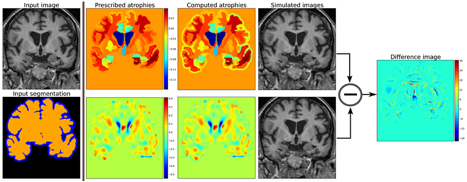
Figure 2. Examples of two different kinds of atrophy maps. The first row prescribes an atrophy map that is uniform in different regions of the brain, while the second row prescribes a smoothly varying atrophy. Both of these atrophy maps have same average values in each ROIs. The example also shows that we can prescribe volume changes in ventricles, if desired, by adapting the input segmentation map accordingly. The simulated images, as shown, are different although they have same mean regional atrophy values. The prescribed atrophy maps and the corresponding computed atrophy maps have different values of atrophy in the regions with sulcal CSF because it is part of Label1 (blue color in the segmentation map) where the volume is allowed to freely change.

2.2. A Biophysical Model of Brain Deformation with Prescribed Volume Changes

Simul@trophy uses the biomechanics based model of brain deformation detailed in Khanal et al. (2016a). The model abstracts the phenomenon that evolves during several months or years in the brain at a macroscopic scale. It is based on the assumption that atrophy creates an internal stress which results in the deformation minimizing a strain energy. In other words, the brain parenchyma deforms with the prescribed atrophy by minimizing the strain energy. The strain energy corresponding to the prescribed atrophy at each time step is completely released when starting the next time step, which leads to a creep flow model.

For a given segmentation image, the model yields a deformation field with the prescribed atrophy at each voxel of Label2 regions (e.g., brain parenchyma). Label1 regions (e.g., the CSF) will correspondingly adapt its volume to globally compensate for the prescribed volume changes in the Label2 regions. For a single time-step, the displacement field u is obtained by solving the system of Equation (1), where Dirichlet boundary conditions of zero deformation are prescribed in Label0 regions.

$\begin{array}{l}\begin{array}{l}\text{Regions with: }\text{L}\text{a}\text{b}\text{e}\text{l}0\\ u=0\\ \text{Dirichlet boundary conditions}\end{array}\}\begin{array}{l}\text{L}\text{a}\text{b}\text{e}\text{l}1\\ \mu \Delta u-\nabla p=0\\ \nabla ·u+kp=0\end{array}\}\\ \begin{array}{l}\text{L}\text{a}\text{b}\text{e}\text{l}2\\ \mu \Delta u-\nabla p=(\mu +\lambda )\nabla a\\ \nabla ·u=-a\end{array}\}& (1)\end{array}$

The system of Equation (1) shows that the incompressibility constraint is relaxed in Label1 regions, while it is strictly satisfied in Label2 regions.

The prescribed atrophy map a in the constraint ∇ · u = −a is the amount of atrophy in a small time step Δt such that the displacement field u and its gradient are small enough to make the following approximation: ∇ · u = −a ≈ J − 1, where J is the Jacobian determinant (Khanal et al., 2016a). Jacobian determinant measures the relative volume of a warped voxel, V₁/V₀.

The impact of the choice of different values for the model parameters μ, λ, and k are detailed in Khanal et al. (2016a). For the same prescribed volume changes, we can obtain different deformation fields by varying these model parameters. In this work, we focus on generating ground truth images with known volume changes and not necessarily generating the exact evolution of the AD patients. Hence, we set the model parameters as follows unless specified otherwise: μ = 1 kPa, λ = 0 kPa, k = 1 kPa⁻¹.

Once the field u with the prescribed volume changes is obtained from the model as described above by using an input baseline image I_b, we can simulate a synthetic follow-up image I_s as follows:

• Let y = Φ_sim(x) = u + x describe a mapping of a point x in physical space to another point y by applying the transformation corresponding to the dense deformation field Φ_sim, or the displacement field u.

• Let Φ_sim⋆I_b describe an action of the diffeomorphism Φ_sim on the image I_b. Thus, the new synthetic image I_s, obtained by warping I_b with the deformation field Φ_sim is given by:

$I_s={\Phi }_{\text{sim}}\star I_b=I_b\circ {\Phi }_{\text{sim}}^{-1}.$

Figure 2 shows two simulated images from the same input baseline image but with two different atrophy patterns.

2.3. Adding Realistic Intensity Variation to Synthetic Longitudinal MRIs

In realistic scenarios, longitudinal MRIs are taken at multiple scan sessions often with slightly different acquisition parameters or even with different scanners. For generating more realistic synthetic longitudinal MRIs, variations in intensity, and noise present in real longitudinal MRIs must also be simulated. If multiple repeat scans of a subject are available, we can use them to simulate such variations in synthetic longitudinal sequences. Assuming that all the available scans of the subject are already aligned using affine registration, this section explains the proposed method of adding realistic variations in the intensity characteristics.

Starting from an input baseline image I_b0 of a subject, the previous sections explained how we can obtain a deformation field Φ_sim from the brain deformation model, and use it to simulate a follow-up image

$I_{s_0}={\Phi }_{\text{sim}}\star I_{b_0}.$

I_s0 has the same intensity characteristics as I_b0, and the intensity noise in I_s0 is strongly correlated to the noise present in I_b0.

If I_b1 is another scan of the same subject taken on the same day, we can obtain a new simulated image by resampling the intensity from I_b1, but still using the same Φ_sim:

$I_{s_1}={\Phi }_{\text{sim}}\star I_{b_1}$

The realistic variation of intensity and artifacts present between the two real scans I_b0 and I_b1 are now also present between the real baseline image I_b0 and the simulated follow-up image I_s1.

The above approach assumes that the brain has not undergone any morphological changes between the scan sessions of the two real images. If the scan time-points of the two images are too far apart to have this assumption valid, we can no longer directly apply Φ_sim to the second image. Let I_r be another real scan of the patient taken at a time later than that of the baseline image I_b0. There might be some morphological changes (e.g., atrophy) in I_r compared to I_b0.

To simulate a new synthetic image with the same atrophy as that of I_s0 but with the intensity resampled from I_r, we must first perform a non-rigid registration between I_r and I_b0. If Φ_reg is the deformation field obtained from the non-rigid registration between I_r and I_b0, it can be used to get an image Φ_reg⋆I_r which is aligned to I_b0. In the ideal case, Φ_reg⋆I_r and I_b0 are perfectly aligned with the only differences lying in the intensity characteristics and the noise.

We can now compose the deformation fields Φ_sim and Φ_reg to generate a new synthetic image as follows:

$I_{s_2}=\left({\Phi }_{\text{sim}}\circ {\Phi }_{\text{reg}}\right)\star I_r.$

I_s2 has the same atrophy as that of I_s0 but with the intensity characteristics of I_r. Figure 3 illustrates how we obtain I_s0, I_s1, and I_s2. These three simulated images have the volume changes as encoded by Φ_sim, but have intensity characteristics coming from three different real images of the same patient.

FIGURE 3

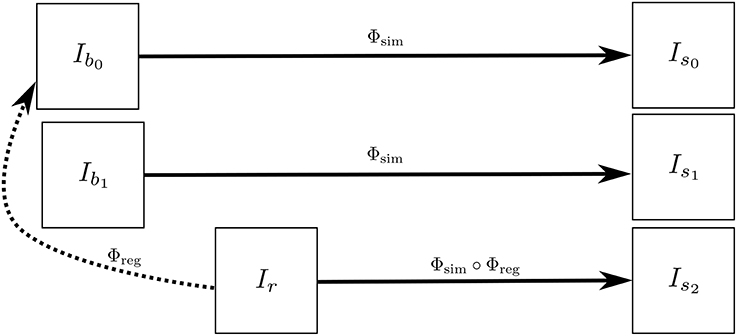
Figure 3. I_b0 and I_b1 are the repeat scans of a subject taken within a short period of time during which there is no morphological changes in the brain of the subject. I_r is taken at a later time when the brain could have undergone some morphological changes. The deformation field Φ_reg is obtained by registering I_r to I_b0, while Φ_sim is obtained from the brain deformation model using I_b0 as the input image. The three simulated images I_s0, I_s1, and I_s1 are all same time-point images but have different intensities that come from I_b0, I_b1, and I_r, respectively.

Figure 4 illustrates how the approach described in this section can be used to generate multiple sets of longitudinal simulated sequences having identical morphological evolution but different variations of intensities. The three shaded regions in Figure 4 are the sets of longitudinal sequences with identical volume changes but with different variations of intensities.

FIGURE 4

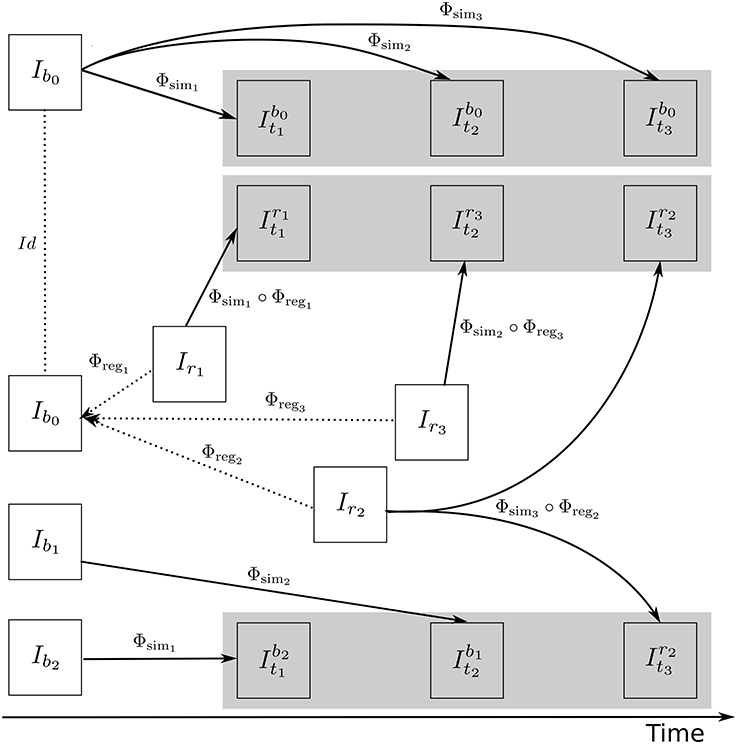
Figure 4. A general approach to simulate ground truth synthetic longitudinal images with realistic intensity variations; simulated images are shown within the shaded regions. The deformation fields with a prescribed atrophy for three time-points (Φ_sim1, Φ_sim2, and Φ_sim3) are obtained from the biophysical model using I_b0 as the input baseline image. Several different sets of longitudinal images can then be simulated by resampling intensities from different combinations of available real images. The topmost shaded region shows a longitudinal sequence with no realistic intensity variations where the synthetic images are all resampled from I_b0. The remaining two shaded regions have longitudinal sequences with realistic intensity variations where the simulated images are resampled from other available images of the same subject. In the ideal case, the three sets of longitudinal sequences have exactly the same morphological changes but with different variations in intensity characteristics.

3. Simulation Examples with Simul@trophy

This section presents simulation examples of synthetic longitudinal MRIs with prescribed atrophy patterns and realistic intensity variations². The real input MRIs used for the simulations presented in this section come from the database made available by Hadj-Hamou et al. (2016). The images had already undergone the Pre-Processing and Position Correction steps of the Longitudinal Log-Demons Framework (LLDF) detailed in Hadj-Hamou et al. (2016). Starting from the publicly available OASIS dataset (Marcus et al., 2010), the images in the database had undergone intensity inhomogeneity correction using ANTs–N4BiasFieldCorrection (Avants et al., 2011), and had been transported to a common space using affine registration with FSL–FLIRT (Jenkinson and Smith, 2001).

Since all the simulated images must undergo interpolation of intensities, numerical scheme used in the interpolation will have an impact on the intensity characteristics of the simulated images. In all the simulation examples that follows, intensities were resampled using B-spline interpolation of order 3.

Figure 5 shows a simulation example where uniform atrophy patterns are prescribed in the hippocampi, the gray matter (GM), and the white matter (WM) regions. The ventricles and sulcal CSF regions are allowed to expand as required to compensate for the volume loss in the brain parenchyma. The figure shows two simulated images whose intensities are resampled from two different images: (i) the input baseline image I_b, (ii) another follow-up image of the same subject, I_r. The figure also shows intensity histograms of these two simulated images for a selected ROI. The selected ROI is a 2D WM region where the simulated images do not have a distinct morphological changes from I_b. Thus, the differences in the intensity histograms of I_b and the simulated images for this ROI is mostly due to the variation in intensity characteristics of the different images. We can see from the figure that the intensity characteristics of the simulated image resampled from I_b closely matches the intensity characteristics of I_b. And resampling the intensity from a different image I_r of the same subject allows simulating realistic variation of intensities.

FIGURE 5

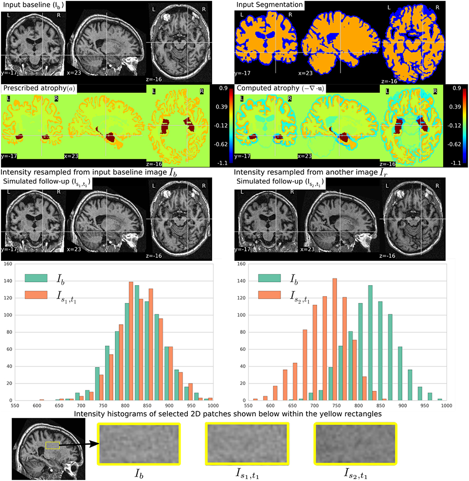
Figure 5. Two simulated images are shown on the third row where the image on the left is resampled from the input baseline image I_b, and the image on the right is resampled from another image I_r of the same subject. Both I_b and I_r had already been corrected for the bias field intensity inhomogeneity. The intensity histograms shown are of a selected ROI (shown on the last row) where there is no significant morphological changes between the images. From the histograms we can see that the simulated image I_{s2, t1} has a different intensity characteristics than I_b, while the simulated image I_{s1, t1} has intensity characteristics that closely matches to that of I_b.

To simulate multiple time-point images, the following approach can be used:

• Get u₀ by solving the system of Equation (1) using the initial atrophy map a₀ and the initial segmentation image L₀ as input.

• For each time step t = 1 to n:

- Warp a_t−1 and L₀ using u_t−1 ∘ u_t−2… ∘ u₀ to get a_t and L_t, respectively.

- Solve for u_t using a_t and L_t as input.

Once all the deformation fields Φ_si corresponding to u_i for i = 0, 1, …, n are obtained, these deformation fields can be used as shown in Figure 4 to simulate different sequences of longitudinal images. As time step gets larger, the segmentation map is warped with an increasingly bigger displacement field using nearest neighbor interpolation, which could result in numerical instabilities. As the atrophy map is also warped at each time step, the global atrophy rate prescribed in the beginning is not necessarily preserved during the intermediate time-steps.

In Figure 6, a simulation example of two longitudinal sequences each having three new time-point images is shown. Both sequences were simulated by prescribing a smoothly varying atrophy pattern. The smoothly varying atrophy pattern prescribed in this example is more complex than the simple pattern used in the previous example. In brain parenchyma regions, it is the negative of the divergence of a stationary velocity field obtained by performing LCC log-Demons registration (Lorenzi et al., 2013) of the input baseline image with a follow-up image of the same subject. The first sequence consists of all the images whose intensities are resampled from the same input baseline image I_b, while the second sequence consists of the images whose intensities are resampled from different real MRIs of the same subject. Thus, as shown in Figure 7, the first sequence does not have the realistic variation of intensities while the second sequence has the realistic variation of intensities. With this example, we also illustrated that we can generate multiple sequences of longitudinal images with same atrophy patterns but different variations of intensities.

FIGURE 6

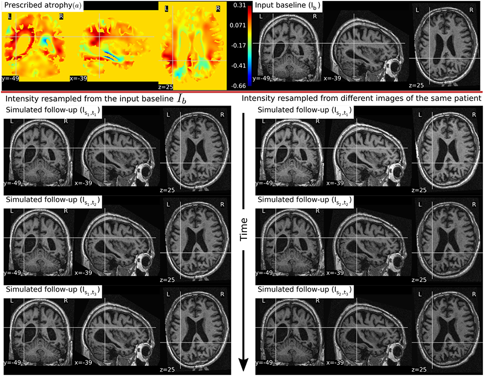
Figure 6. Two sets of synthetic longitudinal images are shown which are simulated by prescribing a smoothly varying atrophy pattern. The first row shows the input prescribed atrophy and the input baseline image I_b of a subject, while the remaining rows show the two sequences. The sequence shown on the left have simulated images that are all resampled from I_b. On the right, each simulated image is resampled from real MRIs of the same subject but taken at different times (at 0.68, 1.77, and 3.3 years after the baseline scan respectively). As shown by the intensity histograms of Figure 7, the longitudinal synthetic images on the right have more realistic intensity variations than the one left.

FIGURE 7

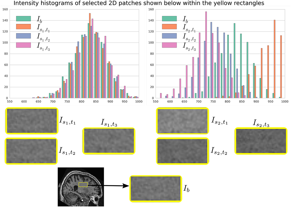
Figure 7. Intensity histograms of selected patches of the images simulated in Figure 6. When the simulated images are resampled from the same input baseline image I_b, as expected, the histograms of the simulated images closely match with each other. However, when simulated images are resampled from other different images of the same patients, the histograms of these simulated images do not match closely. The longitudinal sequence of simulated images I_{s2, t1}, I_{s2, t2}, and I_{s2, t3} has realistic variation in intensities as observed in the real sequences.

Figure 8 shows a simulation example where we prescribe growth instead of atrophy in the brain tissue. The prescribed atrophy in this case is the negative of the atrophy map prescribed in Figure 6. From the segmentation image shown in Figure 8, we can see that the ventricles were allowed to adapt the volume changes as required to compensate for the volume changes in the brain parenchyma. From the three simulated time-points, we can see that these ventricles are shrinking and the brain parenchyma regions are expanding. The example shows that Simul@trophy can be used to simulate images of not only future time-points, but also the past time-point images.

FIGURE 8

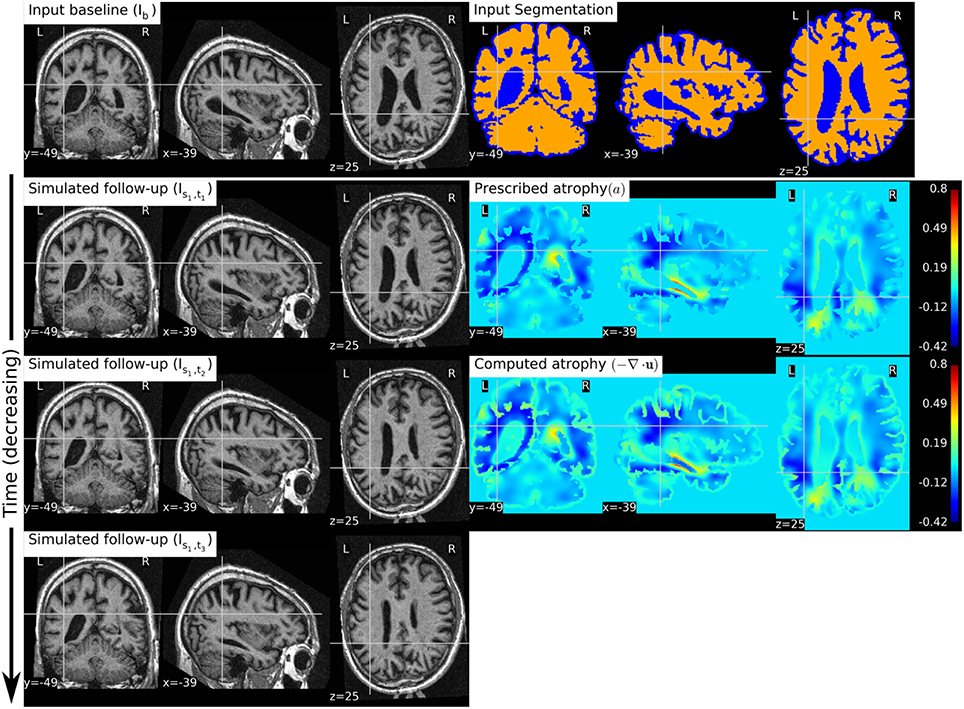
Figure 8. The figure shows an example of simulating a longitudinal sequence with backward time-points. The input baseline image I_b is the same one as used in Figure 6, and the prescribed atrophy map is the negative of the map used in Figure 6. In the figure, we can see the shrinkage of the ventricles and the growth of the brain parenchyma.

In Figure 9, we show an example where synthetic sequence of images is simulated by starting from a baseline image of a healthy subject. However, the prescribed atrophy is derived from an atrophy estimated from the AD patient used in Figure 6. The input baseline images of both the AD patient and the healthy subject were segmented using FreeSurfer (Fischl et al., 2002). In all the segmented regions including the white matter parcellations of the AD patient, the average values of the smoothly varying atrophy map were computed. These regional average values of the atrophy computed from the AD patient were then transported to the corresponding regions of the healthy subject. Thus, in Figure 9, we can see that the prescribed atrophy is region-wise uniform instead of smoothly varying. For comparison, the figure also shows three real time-point images of the healthy subject along with the three simulated time-point images with atrophy derived from the AD patient.

FIGURE 9

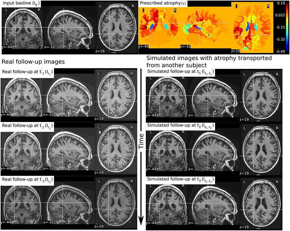
Figure 9. The figure shows an example of simulating follow-up images of a normal subject with baseline image I_b, where the prescribed atrophy pattern is adapted from an AD patient. The prescribed atrophy is adapted from the atrophy estimated for the AD patient shown in Figure 6. Average values of the smoothly varying prescribed atrophy shown in Figure 6 is computed in all the ROIs. The ROIs are obtained from the FreeSurfer segmentation including all the white matter parcellations (Fischl et al., 2002). The simulated images on the right have bigger shrinkage of the brain parenchyma and bigger expansion of the ventricles than the real images on the left.

4. Simul@trophy: Choices Available and Practical Considerations

Simul@trophy is available as an open-source repository under git version control. Researchers can use it according to their needs, improve the presented model, and/or add new models of brain atrophy. It is based on two core components: (i) The Insight ToolKit (ITK) and (ii) PETSc Balay et al. (2013). All the input and output images of the brain deformation model shown in Figure 1 can be in any format that ITK supports. ITK has strongly promoted reproducible science in the medical imaging domain, and has been widely used in computational science applied to medical imaging (McCormick et al., 2014; Avants et al., 2015). Similarly, implementation of the model solver is based on open-source PETSc, a library based on C programming language. It has also been very widely used in a very diverse set of applications that also include the medical field. It is a very powerful library that supports wide range of iterative solvers and preconditioners for large systems of equations. The solvers implemented in PETSc can scale very well to large distributive computer systems.

Simul@trophy runs from command lines where the required inputs and optional choices are provided via command line arguments. The available command lines are detailed in Appendix in Supplementary Material. In this section, we illustrate some examples of how certain choices made during the simulation affect output results.

4.1. Impact of Registration on Simulated Images

In Section 2.3, we explained that starting from an input baseline image of a subject, I_b, we can generate two synthetic images:

$I_{s_1}={\Phi }_{\text{sim}}\star I_f\text{and }{I}_{s_2}=\left({\Phi }_{\text{sim}}\circ {\Phi }_{\text{reg}}\right)\star I_f$

where Φ_sim is the deformation field obtained from the brain deformation model using I_b as the input baseline image, and Φ_reg is the deformation field obtained from the non-rigid registration between I_b and a real follow-up image I_f. Perfect alignment of the two images with a non-rigid registration is possible only in the ideal case scenario. In such an ideal case, the simulated images I_s1 and I_s2 have identical shapes of the brain structures with the only differences lying in the intensity characteristics. In practice, this is almost never the case, and we present below an example of the impact of registration result on the simulated images.

Let us use the following short notations for various images described in this section.

• RB: Real baseline image: I_b,

• RF: Real follow-up image: I_f,

• RB_to_RF: Real baseline aligned to real follow-up: ${\Phi }_{\mathrm{\text{reg}}}^{-1}\star I_b$,

• SF_in_RB: Simulated follow-up image with intensity resampled from I_b: Φ_s⋆I_b,

• SF_in_RF: Simulated follow-up image with intensity resampled from I_f: (Φ_s ∘ Φ_reg)⋆I_f.

Figure 10 illustrates the impact of registration result Φ_reg on the simulation results. The figure shows both the registration and simulation results along with zoomed patches of RB, RB_to_RF, SF_in_RB, and SF_in_RF. As expected, SF_in_RB and SF_in_RF have different intensity characteristics coming from RB and RF, respectively. In the regions where registration is accurate, the two simulated images look almost identical except for the differences in the intensity characteristics. However, in the regions where registration is not accurate enough, SF_in_RB and SF_in_RF do not have identical shapes as expected. Thus, for the proposed method of using deformations obtained by registration for simulation, it might be preferable to use aggressive non-linear registrations with a much bigger weight given to similarity terms than the regularization terms.

FIGURE 10

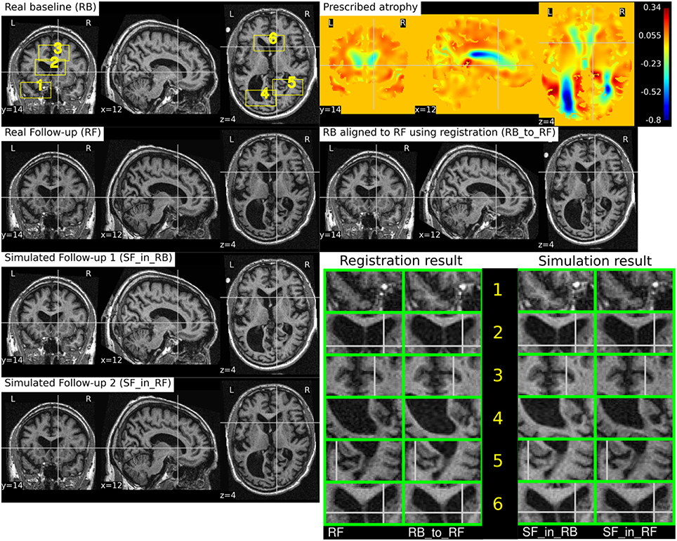
Figure 10. RB and RF are non-rigidly registered and the transformation obtained from the registration is used to align RB to RF which is shown in the image RB_to_RF. The figure also shows two simulated follow-up images SF_in_RB and SF_in_RF that are resampled from (RB) and (RF), respectively. We can see that in most regions of the brain, the two simulated images have almost identical morphological appearances. However, there are also regions such as 2 and 5, where the morphological appearances of the two simulated images are not identical. From the registration results for these regions 2 and 5 in the zoomed patches, we can see that the registration is also not accurate in those regions.

4.2. Discretization Scheme for the Divergence Computation

In Khanal et al. (2016a), a standard staggered grid discretization was used for solving the system of Equation (1). The discretization scheme is shown in Figure 11 in 2D for illustration; explanation on 2D extends naturally to 3D. In the figure, we can see that the components of the displacement field variable u lie on cell faces and not at cell centers. However, all the input and output images for the model, including the output displacement field image, are standard images that have their values lying in cell centers or voxels. Our implementation of the solver internally creates the required staggered grid for the given input images. Once u is computed within the solver of system of Equation(1), its values at cell faces are interpolated to obtain the values at cell centers which are then assembled to send as output displacement field image. Within the solver, the numerical scheme used for the discretization of ∇ · u = −a is:

$\begin{array}{l}\frac{u_{i+1/2,j,k}-u_{i-1/2,j,k}}{h_x}+\frac{v_{i,j+1/2,k}-v_{i,j-1/2,k}}{h_y}+\\ \frac{w_{i,j,k+1/2}-w_{i,j,k-1/2}}{h_z}=a_{i,j,k}& (2)\end{array}$

where,

$u=\left(\begin{array}{c}u\\ v\\ w\end{array}\right).$

FIGURE 11

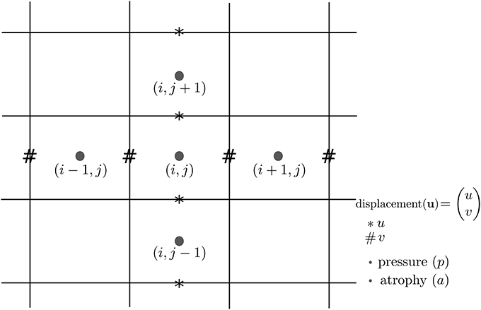
Figure 11. Standard staggered grid discretization scheme that is used to solve the system of Equation (1). Displacement variables are at faces (edges in 2D) of the cells, while pressure and atrophy values are at centers of the cells.

Simul@trophy then provides output displacement field image with the values of u lying at cell centers or voxels by using linear interpolation as follows:

$\begin{array}{ll}\left(\begin{array}{c}{u}_{i,j,k}\\ v_{i,j,k}\\ w_{i,j,k}\end{array}\right)=\left(\begin{array}{c}\left(u_{i+1/2,j,k}+u_{i-1/2,j,k}\right)/2\\ \left(v_{i,j+1/2,k}+v_{i,j-1/2,k}\right)/2\\ \left(w_{i,j,k+1/2}+w_{i,j,k-1/2}\right)/2\end{array}\right)& (3)\end{array}$

To compare divergence maps of this output field with the ones obtained from tools external of Simul@trophy, the only accessible values are the interpolated ones. ITK is widely used in registration based brain morphometry algorithms, but the default derivative computation of ITK has the following centered difference stencil:

$\begin{array}{ll}\frac{u_{i+1,j,k}-u_{i-1,j,k}}{2*h_x}+\frac{v_{i,j+1,k}-v_{i,j-1,k}}{2*h_y}+\frac{w_{i,j,k+1}-w_{i,j,k-1}}{2*h_z}=a_{i,j,k}& (4)\end{array}$

Replacing the components of u at cell centers from Equation 3, we get,

$\begin{array}{ll}\frac{u_{i+3/2,j,k}+u_{i+1/2,j,k}-(u_{i-1/2,j,k}+u_{i+3/2,j,k})}{4*h_x}+...=a_{i,j,k}& (5)\end{array}$

The scheme in Equation (5) does not match the one that was used internally by Simul@trophy shown in Equation (2). This results in discrepancy if we compare input prescribed atrophy maps against the externally computed divergence maps ∇ · u. Thus, in this work, we have added an implementation for the scheme in Equation (5) so that users can choose either of the two possible schemes of Equations (2, 5). The latter scheme is consistent with the divergence computed by the default derivative computation options of ITK. At each 3D cell, the scheme in Equation (2) involves 6 variables of the displacement field, while the scheme in Equation (5) involves 12 variables. In the rest of the paper, they will be referred to as 6-point and 12-point schemes, respectively.

Figure 12 shows the error in specified vs. obtained atrophy when using the two different numerical schemes. As expected, we can see that when a consistent numerical scheme is used, there is no difference between the specified and obtained atrophy. When the schemes are not consistent, the error is larger on the areas where the prescribed atrophy values change sharply.

FIGURE 12

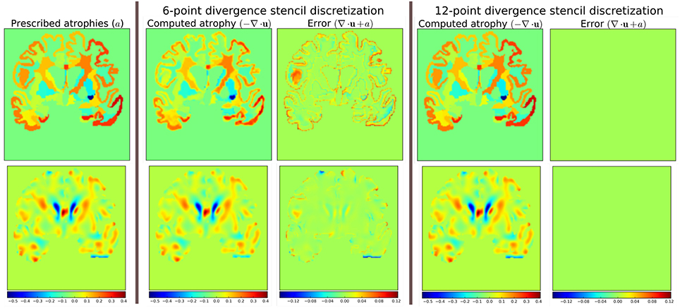
Figure 12. Error due to non-consistent numerical schemes in Equations (2, 4, 5). ∇ · u shown in the figure are computed external of Simul@trophy by using the default ITK derivative computation scheme shown in Equation (4). When this divergence computation is consistent with the one used in Simul@trophy, we should obtain zero error with ∇ · u + a = 0. This is indeed the case, as seen on the right, when we use 12-point stencil of Equation (5). We see non-zero errors when using 6-point stencil from Equation (2) because this scheme and the default ITK scheme are not consistent. The figure shows that the error gets larger at areas where prescribed atrophy has discontinuous jumps.

If the simulated ground truth images using Simul@trophy are used for the evaluation of atrophy estimation algorithms, one must also be careful about the measure of volume change used in addition to the numerical scheme used. For instance, many TBM based brain morphometry algorithms use Jacobian determinants as a measure of volume change. To compute ground truth volume changes of the simulated images for the evaluation of such algorithms, users should compute Jacobian determinants using the same numerical scheme as used by the atrophy estimation algorithm being evaluated. For instance, if multiple time-steps was used in simulating the final image then the Jacobian must be computed at each individual step and properly accumulated to get the final volume change.

4.3. Implementation of Image Warping

When implementing an algorithm to warp an image with a given deformation field, it is more convenient to use the inverse of the deformation field. If Φ_s is the output deformation field obtained from the brain deformation model by using I_b as the input baseline image, Φ_s maps any point x in I_b to a point y in the simulated image I_s as follows:

$y={\Phi }_s(x).$

However, y is not guaranteed to be a discrete voxel location. Since we do not know the intensity values of I_s a priori in the nearby discrete positions, the problem of interpolation is much more complex. Thus, we start from a discrete voxel location y in I_s where the value of intensity is to be found. Then, the corresponding position x in I_b can be obtained by using the inverse deformation field:

$x={\Phi }_s^{-1}(y).$

If the transformed point x is not a discrete point, we can interpolate the intensities of I_b from neighboring discrete locations. Let us denote the interpolation by square brackets. Thus, i = I[x] describes a mapping of a point x to an intensity, i, of the MR image I at x. Using this notation, the intensity of the simulated image at any position x is given by:

$I_b\left[{\Phi }_s^{-1}(x)\right].$

The following option can be used to invert the deformation field:

--invert_field_to_warp $\#\text{Invert}$u;

      $\text{default}:\text{ do not invert}$

The implementation of the inversion is adapted from a fixed-point scheme implementation available in ITK (Luethi, 2010). By default, the simulator uses B-spline interpolation of order three to warp the input images.

4.4. Standalone Utility Tools and Scripts for Pre-processing and Post-processing

There are some standalone tools and scripts available for various pre- and post-processing operations that are detailed in the documentation of the released software.

Some of these tools for pre-processing and post-processing operations are C++ executables based on ITK, while others are python scripts. In this work, all the input segmentation of the model were obtained by using FreeSurfer. As explained in Khanal et al. (2016a), these segmentation maps were processed to obtain in the format required by the model. Although the provided scripts are developed for FreeSurfer segmentation maps, they can be easily modified to adapt to other pre-processing tools. Finally, the registration and simulation deformations were composed using ComposeMultiTransform of Advanced Neuroimaging Tools (ANTs) (Avants et al., 2011).

The core component of Simul@trophy is the implementation of the brain deformation model. Resampling of the intensity is straightforward once the deformations from the model and from registration are available. The simulator is not dependent on any one particular registration algorithm. Although, we used LCC-LogDemons for illustrative purposes, this can be replaced with any other non-rigid registration algorihtms. Similarly pre-processing is also independent of Simul@trophy. We used FreeSurfer in the simulation examples shown in this work, but any other skull stripping and segmentation algorithms can be used. Simul@trophy provides some example scripts and some utility scripts, which could be modified when using other tools for the pre-processing step.

5. Discussion

In Khanal et al. (2016a), we presented a method to generate a subject-specific atrophy pattern by first measuring the atrophy from the available time-points, and then simulating a new time-point by prescribing the measured atrophy. In Khanal et al. (2016b), we extended the method to interpolate an unavailable intermediate time-point MRI. In this work, we added realistic variation in the intensity of the synthetic images. This fills an important gap in the existing literature to simulate atrophy in longitudinal images with realistic intensity variation without explicitly modeling the noise and acquisition artifacts. The simulation examples were shown using three types of atrophy patterns: (i) very simple uniform volume changes in small number of regions, (ii) uniform atrophy in large number of regions, and (iii) smoothly varying atrophy patterns.

For each subject, we could generate large number of synthetic images by perturbing these atrophy patterns in different ways. Even with the same atrophy pattern, we can generate multiple sets of longitudinal sequences of varying intensity characteristics using the approach illustrated in Figure 4. Thus, by changing the atrophy patterns and the image intensities, Simul@trophy could be used to generate a database of very large number of simulated images. Such a database might be useful for training of machine learning algorithms.

In Figure 6, smoothly varying atrophy pattern was prescribed by taking the negative of the divergence of a stationary velocity field obtained by registering the input baseline image with a follow-up image of the same subject. The objective of the experiment was to illustrate the ability of Simul@trophy to simulate smoothly varying patterns of atrophy in addition to the piecewise continuous atrophy maps. Registration was taken just as a means of getting a realistic smoothly varying atrophy maps; it is worth mentioning that simulating the deformation to be close to the deformation obtained from the registration algorithm was not the objective of this experiment. This is because the actual deformation field depends on the regularization used in the registration algorithm which does not necessarily follow the modeling assumptions used by Simul@trophy.

Although, the proposed method of resampling intensity from an image different from the input image provides more realistic variations, there are nevertheless certain issues one needs to be aware of. Since the simulated image has its intensities interpolated from another image, it can slightly reduce the noise variance. A neighborhood with expansion in the simulated image have intensities with slightly different linear combinations of intensities coming from a smaller set of voxels in the input image. Thus, the simulated image would have a smoother autocorrelation in the neighborhood compared to an equivalent real image. The fact that the simulated image has undergone interpolation and draws intensities from a limited set of raw voxels means that it is inherently smoother than the real scans. Finally, the usual spatial patterns of artifacts on real scans might not be exactly reproduced when warping real images. Any application using the simulated sets of images with the proposed approach should be aware of and ideally take into account these issues when interpreting results.

Use of repeat baseline scans to obtain intensity variation in the simulated images provides a very simple approach without using explicit noise and artifact models. One limitation with this is that the repeat baseline scans are not always available. When repeat scans are not available, we have proposed to use images at other time-points of the same subject, which requires performing non-linear registration. However, none of the non-linear registration methods are perfect and therefore the inaccuracies in registration affect the simulation results. This issue was discussed with illustrative examples in Section 4.1.

Simul@trophy can be used in evaluating atrophy estimation algorithms in similar ways as done by Pieperhoff et al. (2008), Camara et al. (2008), and Sharma et al. (2010). Since the proposed approach to simulate images may need deformations estimated from image registration, the use of these simulated images for the evaluation of some registration algorithms can bring an issue of circularity. This limitation adds to another limitation present in all publications related to atrophy simulation that we are aware of: namely, the models used in simulating images could favor certain kinds of registration algorithms over others. Although the ground truth atrophy can be measured from the combined deformation fields, the users must be aware of both limitations when they use Simul@trophy for the evaluation of registration algorithms.

The ability to prescribe atrophy at any time point allows the user to introduce volume changes at different regions of the brain at different times. Thus, another interesting application of the simulator is to train and/or validate disease progression models such as the models proposed in Chen et al. (2012), Fonteijn et al. (2012), Jedynak et al. (2012), Dukart et al. (2013), and Schmidt-Richberg et al. (2016). Having a database of longitudinal MRIs with known spatio-temporal distribution of atrophy can be useful to validate such algorithms. Furthermore, since the algorithms use a data driven approach, the simulator could be useful to train or fine-tune such models.

Another possible application is in filling up unavailable time-point MRIs of some of the subjects, when performing group-wise longitudinal analysis. In such studies, usually the available time-point images of each subject are used to estimate subject-specific volume changes. These subject-specific measurements are then used to perform group-wise statistics to check whether there are significant differences amongst different groups in some particular regions of the brain. Databases used in such analyses, might not always have all the required time-point images for all the subjects. This could lead to bias if all the subjects are not aligned properly in the temporal dimension of disease progression. Simulating new time-point images for some subjects and using them in the analysis might allow evaluating the impact of such mis-alignments.

Simul@trophy could also be used in studying the role of morphology and intensity on atrophy estimation algorithms, and in machine learning based AD classification algorithms. Simul@trophy enables to perform such studies as it allows creating a large number of images by simulating atrophy patterns commonly observed in AD patients but with intensities taken from normal subjects and vice versa.

We hope to promote two directions of research in the community with open-source release of Simul@trophy. First, the public availability of Simul@trophy enables researchers to build their own simulated databases as needed. This might also hopefully lead to a large public database of ground truth simulated images, that could be used for benchmarking and evaluation of various image based morphometry tools. Second, we hope that Simul@trophy allows other researchers to build upon the biophysical model we presented in Khanal et al. (2016a), and investigate further, providing more accurate models of brain atrophy.

Finally, Simul@trophy is general enough to be used for other imaging modalities such as CT scans. It could also be used with images of any other organs, where one requires simulating specified volume changes. In this case, the pre-processing should be changed accordingly to generate a segmentation image and atrophy maps. Thus, once the software is public, other researchers might find it useful in applications that we have not foreseen yet.

6. Conclusions

We proposed a simulation framework that can generate realistic longitudinal MRIs with specified volume changes. The framework allows generating large number of subject-specific multiple time-point images based on a biophysical model of brain deformation due to atrophy. We developed an open-source software Simul@trophy to implement the proposed framework. The core part of Simul@trophy is the implementation of our brain deformation model presented in Khanal et al. (2016a). Simul@trophy is based on widely used state of the art libraries PETSc (for solving large systems of equations) and ITK (for medical image processing). Since the software is publicly available in an open-source repository, we hope that researchers can use it to create databases of ground truth images. The framework could be used to generate a common public database, which in turn could be used to validate and evaluate a large number of available atrophy estimation algorithms. Similarly, these databases could be valuable for data driven disease progression models including machine learning algorithms. Validation and training of the models that study temporal relationships, ordering, and co-evolution of atrophy in different structures of the brain could be another interesting application.

Author Contributions

BK has worked on the design and implementation of Simul@trophy. NA and XP have supervised him in the design of the experiments and in the methods presented in the paper. BK has written the manuscript with multiple iterations of suggestions and corrections from NA and XP.

Funding

Part of this work was funded by the European Research Council through the ERC Advanced Grant MedYMA 2011-291080.

Conflict of Interest Statement

The authors declare that the research was conducted in the absence of any commercial or financial relationships that could be construed as a potential conflict of interest.

Acknowledgments

1. We would like to thank Mehdi Hadj-Hamou for providing us registration results and the associated deformation fields that were used in this paper to resample intensity from different images. The preprocessing steps involved for this registration are explained in Hadj-Hamou et al. (2016).

2. Most part of this work has first appeared in the Ph.D. thesis of BK (Khanal, 2016), and the publication of content from the Ph.D. thesis is in line with author's university policy. A previous version of this paper has been archived as a preprint on Hal (https://hal.inria.fr/hal-01348959v1). The authors hold the copyrights on both of these.

3. Part of this work was funded by the European Research Council through the ERC Advanced Grant MedYMA 2011-291080.

4. This work benefited from the use of the Insight Segmentation and Registration Toolkit (ITK), an open source software developed as an initiative of the U.S. National Library of Medicine and available at www.itk.org.

5. The multi-platform configuration tool CMake was used for configuring ITK and facilitating its use from our project. CMake was partially funded by the U.S. National Library of Medicine as part of the Insight Toolkit project. CMake is an open source system and it is freely available at www.cmake.org.

Supplementary Material

The Supplementary Material for this article can be found online at: http://journal.frontiersin.org/article/10.3389/fnins.2017.00132/full#supplementary-material

Footnotes

1. ^Available at: https://inria-asclepios.github.io/simul-atrophy/.

2. ^The simulation results are made available at http://neurovault.org/collections/AUKWWYBC/ (Gorgolewski et al., 2015).

References

Ashburner, J. (2013). Symmetric diffeomorphic modeling of longitudinal structural MRI. Front. Neurosci. 6:197. doi: 10.3389/fnins.2012.00197

PubMed Abstract | CrossRef Full Text | Google Scholar

Ashburner, J., and Friston, K. J. (2000). Voxel-based morphometry–the methods. NeuroImage 11, 805–821. doi: 10.1006/nimg.2000.0582

PubMed Abstract | CrossRef Full Text | Google Scholar

Ashburner, J., and Ridgway, G. R. (2015). “Tensor-based morphometry,” in Brain Mapping: An Encyclopedic Reference, ed A. W. Toga (Academic Press; Elsevier), 383–394.

Google Scholar

Avants, B., Johnson, H. J., and Tustison, N. J. (2015). Neuroinformatics and the the insight toolkit. Front. Neuroinform. 9:5. doi: 10.3389/fninf.2015.00005

PubMed Abstract | CrossRef Full Text | Google Scholar

Avants, B. B., Tustison, N. J., Song, G., Cook, P. A., Klein, A., and Gee, J. C. (2011). A reproducible evaluation of ants similarity metric performance in brain image registration. NeuroImage 54, 2033–2044. doi: 10.1016/j.neuroimage.2010.09.025

PubMed Abstract | CrossRef Full Text | Google Scholar

Balay, S., Brown, J., Buschelman, K., Gropp, W. D., Kaushik, D., Knepley, M. G., et al. (2013). PETSc Web Page. Available online at: http://www.mcs.anl.gov/petsc

Camara, O., Schnabel, J. A., Ridgway, G. R., Crum, W. R., Douiri, A., Scahill, R. I., et al. (2008). Accuracy assessment of global and local atrophy measurement techniques with realistic simulated longitudinal Alzheimer's disease images. NeuroImage 42, 696–709. doi: 10.1016/j.neuroimage.2008.04.259

PubMed Abstract | CrossRef Full Text | Google Scholar

Camara, O., Schweiger, M., Scahill, R. I., Crum, W. R., Sneller, B. I., Schnabel, J. A., et al. (2006). Phenomenological model of diffuse global and regional atrophy using finite-element methods. IEEE Trans. Med. Imaging 25, 1417–1430. doi: 10.1109/TMI.2006.880588

PubMed Abstract | CrossRef Full Text | Google Scholar

Camara-Rey, O., Sneller, B. I., Ridgway, G. R., Garde, E., Fox, N. C., and Hill, D. L. (2006). “Simulation of acquisition artefacts in mr scans: effects on automatic measures of brain atrophy,” in International Conference on Medical Image Computing and Computer-Assisted Intervention (Copenhagen: Springer), 272–280.

Google Scholar

Carmichael, O., McLaren, D. G., Tommet, D., Mungas, D., and Jones, R. N. (2013). Coevolution of brain structures in amnestic mild cognitive impairment. NeuroImage 66, 449–456. doi: 10.1016/j.neuroimage.2012.10.029

PubMed Abstract | CrossRef Full Text | Google Scholar

Chen, R., Resnick, S. M., Davatzikos, C., and Herskovits, E. H. (2012). Dynamic bayesian network modeling for longitudinal brain morphometry. NeuroImage 59, 2330–2338. doi: 10.1016/j.neuroimage.2011.09.023

PubMed Abstract | CrossRef Full Text | Google Scholar

Dukart, J., Kherif, F., Mueller, K., Adaszewski, S., Schroeter, M. L., Frackowiak, R. S. J., et al. (2013). Generative FDG-PET and MRI model of aging and disease progression in alzheimer's disease. PLoS Comput. Biol. 9:e1002987. doi: 10.1371/journal.pcbi.1002987

PubMed Abstract | CrossRef Full Text | Google Scholar

Fischl, B., Salat, D. H., Busa, E., Albert, M., Dieterich, M., Haselgrove, C., et al. (2002). Whole brain segmentation: automated labeling of neuroanatomical structures in the human brain. Neuron 33, 341–355. doi: 10.1016/S0896-6273(02)00569-X

PubMed Abstract | CrossRef Full Text | Google Scholar

Fonteijn, H. M., Modat, M., Clarkson, M. J., Barnes, J., Lehmann, M., Hobbs, N. Z., et al. (2012). An event-based model for disease progression and its application in familial Alzheimer's disease and Huntington's disease. NeuroImage 60, 1880–1889. doi: 10.1016/j.neuroimage.2012.01.062

PubMed Abstract | CrossRef Full Text | Google Scholar

Freeborough, P. A., and Fox, N. C. (1997). The boundary shift integral: an accurate and robust measure of cerebral volume changes from registered repeat MRI. IEEE Trans. Med. Imaging 16, 623–629. doi: 10.1109/42.640753

PubMed Abstract | CrossRef Full Text | Google Scholar

Frisoni, G. B., Fox, N. C., Jack, C. R., Scheltens, P., and Thompson, P. M. (2010). The clinical use of structural MRI in Alzheimer disease. Nat. Rev. Neurol. 6, 67–77. doi: 10.1038/nrneurol.2009.215

PubMed Abstract | CrossRef Full Text | Google Scholar

Gorgolewski, K. J., Varoquaux, G., Rivera, G., Schwartz, Y., Ghosh, S. S., Maumet, C., et al. (2015). Neurovault.org: a web-based repository for collecting and sharing unthresholded statistical maps of the human brain. Front. Neuroinform. 9:8. doi: 10.3389/fninf.2015.00008

PubMed Abstract | CrossRef Full Text | Google Scholar

Gudbjartsson, H., and Patz, S. (1995). The Rician distribution of noisy MRI data. Magn. Reson. Med. 34, 910–914. doi: 10.1002/mrm.1910340618

PubMed Abstract | CrossRef Full Text | Google Scholar

Hadj-Hamou, M., Lorenzi, M., Ayache, N., and Pennec, X. (2016). Longitudinal analysis of image time series with diffeomorphic deformations: a computational framework based on stationary velocity fields. Front. Neurosci. 10:236. doi: 10.3389/fnins.2016.00236

PubMed Abstract | CrossRef Full Text | Google Scholar

Hua, X., Leow, A. D., Parikshak, N., Lee, S., Chiang, M.-C., Toga, A. W., et al. (2008). Tensor-based morphometry as a neuroimaging biomarker for Alzheimer's disease: an MRI study of 676 AD, MCI, and normal subjects. NeuroImage 43, 458–469. doi: 10.1016/j.neuroimage.2008.07.013

PubMed Abstract | CrossRef Full Text | Google Scholar

Jedynak, B. M., Lang, A., Liu, B., Katz, E., Zhang, Y., Wyman, B. T., et al. (2012). A computational neurodegenerative disease progression score: method and results with the Alzheimer's disease neuroimaging initiative cohort. NeuroImage 63, 1478–1486. doi: 10.1016/j.neuroimage.2012.07.059

PubMed Abstract | CrossRef Full Text | Google Scholar

Jenkinson, M., and Smith, S. (2001). A global optimisation method for robust affine registration of brain images. Med. Image Anal. 5, 143–156. doi: 10.1016/S1361-8415(01)00036-6

PubMed Abstract | CrossRef Full Text | Google Scholar

Karaçali, B., and Davatzikos, C. (2006). Simulation of tissue atrophy using a topology preserving transformation model. IEEE Trans. Med. Imaging 25, 649–652. doi: 10.1109/TMI.2006.873221

PubMed Abstract | CrossRef Full Text | Google Scholar

Khanal, B. (2016). Modeling and Simulation of Realistic Longitudinal Structural Brain MRIs with Atrophy in Alzheimer's Disease. Theses, Université Nice Sophia Antipolis. Available online at: https://tel.archives-ouvertes.fr/tel-01384678

Khanal, B., Lorenzi, M., Ayache, N., and Pennec, X. (2014). “A biophysical model of shape changes due to atrophy in the brain with Alzheimer's disease,” in Medical Image Computing and Computer-Assisted Intervention; MICCAI 2014, Vol. 8674, Lecture Notes in Computer Science, eds P. Golland, N. Hata, C. Barillot, J. Hornegger, and R. Howe (Boston, MA: Springer International Publishing), 41–48.

Google Scholar

Khanal, B., Lorenzi, M., Ayache, N., and Pennec, X. (2016a). A biophysical model of brain deformation to simulate and analyze longitudinal mris of patients with Alzheimer's disease. NeuroImage 134, 35–52. doi: 10.1016/j.neuroimage.2016.03.061

PubMed Abstract | CrossRef Full Text | Google Scholar

Khanal, B., Lorenzi, M., Ayache, N., and Pennec, X. (2016b). “Simulating patient specific multiple time-point mris from a biophysical model of brain deformation in Alzheimer's disease,” in Computational Biomechanics for Medicine: Imaging, Modeling and Computing, eds G. Joldes, B. Doyle, A. Wittek, P. M. F. Nielsen, and K. Miller (Munich: Springer International Publishing AG), 167–176.

Google Scholar

Koch, K., Reess, T. J., Rus, O. G., and Zimmer, C. (2016). Extensive learning is associated with gray matter changes in the right hippocampus. NeuroImage 125, 627–632. doi: 10.1016/j.neuroimage.2015.10.056

PubMed Abstract | CrossRef Full Text | Google Scholar

Langlois, S., Desvignes, M., Constans, J. M., and Revenu, M. (1999). MRI geometric distortion: a simple approach to correcting the effects of non-linear gradient fields. J. Magn. Reson. Imaging 9, 821–831. doi: 10.1002/(SICI)1522-2586(199906)9:6<821::AID-JMRI9>3.0.CO;2-2

PubMed Abstract | CrossRef Full Text | Google Scholar

Lorenzi, M., Ayache, N., Frisoni, G., and Pennec, X. (2013). LCC-Demons: a robust and accurate symmetric diffeomorphic registration algorithm. NeuroImage 81, 470–483. doi: 10.1016/j.neuroimage.2013.04.114

PubMed Abstract | CrossRef Full Text | Google Scholar

Luethi, M. (2010). Inverting deformation fields using a fixed point iteration scheme. Insight J. Available online at: http://hdl.handle.net/10380/3222

Google Scholar

Marcus, D. S., Fotenos, A. F., Csernansky, J. G., Morris, J. C., and Buckner, R. L. (2010). Open access series of imaging studies: longitudinal MRI data in nondemented and demented older adults. J. Cogn. Neurosci. 22, 2677–2684. doi: 10.1162/jocn.2009.21407

PubMed Abstract | CrossRef Full Text | Google Scholar

McCormick, M. M., Liu, X., Ibanez, L., Jomier, J., and Marion, C. (2014). ITK: enabling reproducible research and open science. Front. Neuroinform. 8:13. doi: 10.3389/fninf.2014.00013

PubMed Abstract | CrossRef Full Text | Google Scholar

Modat, M., Simpson, I. J. A., Cardoso, M. J., Cash, D. M., Toussaint, N., Fox, N. C., et al. (2014). “Simulating neurodegeneration through longitudinal population analysis of structural and diffusion weighted MRI data,” in Medical Image Computing and Computer-Assisted Intervention – MICCAI 2014: 17th International Conference, Boston, MA, USA, Proceedings, Part III, Lecture Notes in Computer Science, eds P. Golland, N. Hata, C. Barillot, J. Hornegger, and R. Howe (Boston, MA: Springer International Publishing), 57–64.

Google Scholar

Pieperhoff, P., Südmeyer, M., Hömke, L., Zilles, K., Schnitzler, A., and Amunts, K. (2008). Detection of structural changes of the human brain in longitudinally acquired MR images by deformation field morphometry: methodological analysis, validation and application. NeuroImage 43, 269–287. doi: 10.1016/j.neuroimage.2008.07.031

PubMed Abstract | CrossRef Full Text | Google Scholar

Prados, F., Cardoso, M. J., Leung, K. K., Cash, D. M., Modat, M., Fox, N. C., et al. (2015). Measuring brain atrophy with a generalized formulation of the boundary shift integral. Neurobiol. Aging 36, S81–S90. doi: 10.1016/j.neurobiolaging.2014.04.035

PubMed Abstract | CrossRef Full Text | Google Scholar

Prakosa, A., Sermesant, M., Delingette, H., Marchesseau, S., Saloux, E., Allain, P., et al. (2013). Generation of synthetic but visually realistic time series of cardiac images combining a biophysical model and clinical images. IEEE Trans. Med. Imaging 32, 99–109. doi: 10.1109/TMI.2012.2220375

PubMed Abstract | CrossRef Full Text | Google Scholar

Preboske, G. M., Gunter, J. L., Ward, C. P., and Jack, C. R. (2006). Common mri acquisition non-idealities significantly impact the output of the boundary shift integral method of measuring brain atrophy on serial MRI. Neuroimage 30, 1196–1202. doi: 10.1016/j.neuroimage.2005.10.049

PubMed Abstract | CrossRef Full Text | Google Scholar

Radua, J., Canales-Rodríguez, E. J., Pomarol-Clotet, E., and Salvador, R. (2014). Validity of modulation and optimal settings for advanced voxel-based morphometry. NeuroImage 86, 81–90. doi: 10.1016/j.neuroimage.2013.07.084

PubMed Abstract | CrossRef Full Text | Google Scholar

Rosen, H. J., Gorno-Tempini, M. L., Goldman, W., Perry, R., Schuff, N., Weiner, M., et al. (2002). Patterns of brain atrophy in frontotemporal dementia and semantic dementia. Neurology 58, 198–208. doi: 10.1212/WNL.58.2.198

PubMed Abstract | CrossRef Full Text | Google Scholar

Schmidt-Richberg, A., Ledig, C., Guerrero, R., Molina-Abril, H., Frangi, A., Rueckert, D., et al. (2016). Learning biomarker models for progression estimation of alzheimer's disease. PLoS ONE 11:e0153040. doi: 10.1371/journal.pone.0153040

PubMed Abstract | CrossRef Full Text | Google Scholar

Sepulcre, J., Sastre-Garriga, J., Cercignani, M., Ingle, G. T., Miller, D. H., and Thompson, A. J. (2006). Regional gray matter atrophy in early primary progressive multiple sclerosis: a voxel-based morphometry study. Arch. Neurol. 63, 1175–1180. doi: 10.1001/archneur.63.8.1175

PubMed Abstract | CrossRef Full Text | Google Scholar

Sharma, S., Noblet, V., Rousseau, F., Heitz, F., Rumbach, L., and Armspach, J. (2010). Evaluation of brain atrophy estimation algorithms using simulated ground-truth data. Med. Image Anal. 14, 373–389. doi: 10.1016/j.media.2010.02.002

PubMed Abstract | CrossRef Full Text | Google Scholar

Sharma, S., Rousseau, F., Heitz, F., Rumbach, L., and Armspach, J. (2013). On the estimation and correction of bias in local atrophy estimations using example atrophy simulations. Comput. Med. Imaging Graph. 37, 538–551. doi: 10.1016/j.compmedimag.2013.07.002

PubMed Abstract | CrossRef Full Text | Google Scholar

Simmons, A., Tofts, P. S., Barker, G. J., and Arridge, S. R. (1994). Sources of intensity nonuniformity in spin ECHO images at 1.5 T. Magn. Reson. Med. 32, 121–128. doi: 10.1002/mrm.1910320117

PubMed Abstract | CrossRef Full Text | Google Scholar

Sled, J. G., Zijdenbos, A. P., and Evans, A. C. (1998). A nonparametric method for automatic correction of intensity nonuniformity in MRI data. IEEE Trans. Med. Imaging 17, 87–97. doi: 10.1109/42.668698

PubMed Abstract | CrossRef Full Text | Google Scholar

Smith, A. D. C., Crum, W. R., Hill, D. L., Thacker, N. A., and Bromiley, P. A. (2003). “Biomechanical simulation of atrophy in MR images,” in Medical Imaging 2003, eds M. Sonka and J. M. Fitzpatrick (San Diego, CA: International Society for Optics and Photonics), 481–490.

Google Scholar

Smith, S. M., Zhang, Y., Jenkinson, M., Chen, J., Matthews, P., Federico, A., et al. (2002). Accurate, robust, and automated longitudinal and cross-sectional brain change analysis. Neuroimage 17, 479–489. doi: 10.1006/nimg.2002.1040

PubMed Abstract | CrossRef Full Text | Google Scholar

Whitwell, J. L., and Jack, C. R. Jr. (2005). Comparisons between Alzheimer disease, frontotemporal lobar degeneration, and normal aging with brain mapping. Top. Magn. Reson. Imaging 16, 409–425. doi: 10.1097/01.rmr.0000245457.98029.e1

PubMed Abstract | CrossRef Full Text | Google Scholar

Wright, I., McGuire, P., Poline, J.-B., Travere, J., Murray, R., Frith, C., et al. (1995). A voxel-based method for the statistical analysis of gray and white matter density applied to schizophrenia. NeuroImage 2, 244–252. doi: 10.1006/nimg.1995.1032

PubMed Abstract | CrossRef Full Text | Google Scholar