Neural field simulator: two-dimensional spatio-temporal dynamics involving finite transmission speed

Neural Field models (NFM) play an important role in the understanding of neural population dynamics on a mesoscopic spatial and temporal scale. Their numerical simulation is an essential element in the analysis of their spatio-temporal dynamics. The simulation tool described in this work considers scalar spatially homogeneous neural fields taking into account a finite axonal transmission speed and synaptic temporal derivatives of first and second order. A text-based interface offers complete control of field parameters and several approaches are used to accelerate simulations. A graphical output utilizes video hardware acceleration to display running output with reduced computational hindrance compared to simulators that are exclusively software-based. Diverse applications of the tool demonstrate breather oscillations, static and dynamic Turing patterns and activity spreading with finite propagation speed. The simulator is open source to allow tailoring of code and this is presented with an extension use case.

1. Introduction

The understanding of spatio-temporal electric activity in neural tissue is essential in the study of neurobiological phenomena. To achieve this, mesoscopic-scale models such as neural mass and neural fields (NFM) which describe the dynamics of a large population of neurons reflecting coarse-grained properties of single neurons (Wilson and Cowan, 1973; Deco et al., 2008; Bressloff, 2012; Hutt and Buhry, 2014) play an important role. NFMs serve as a good description of the dynamic source of Local Field Potentials and encephalographic data (Nunez, 1974, 2000; Wright and Kydd, 1992; Wright and Liley, 1994; Jirsa et al., 2002; Nunez and Srinivasan, 2006; Coombes et al., 2014). They allow to consider diverse single neuron features that may tune neural population dynamics, such as somatic (Molaee-Ardekani et al., 2007) and synaptic adaptation (Coombes and Owen, 2005; Kilpatrick and Bressloff, 2010), extra-synaptic receptor dynamics (Hashemi et al., 2014; Hutt and Buhry, 2014) or finite axonal transmission speed (Jirsa and Haken, 1996; Pinto and Ermentrout, 2001; Hutt et al., 2003, 2008; Coombes, 2005; Faye and Faugeras, 2010; Veltz and Faugeras, 2011, 2013). All these applications make NFMs valuable in order to understand spatio-temporal dynamics of neural population activity.

Mathematical analysis and the numerical integration of NFMs are complementary. The recent years have shown strong attention of research on the mathematical properties of NFMs, whereas the numerical simulation of NFM solutions has been less considered in research. Since NFMs generalize partial differential equations (Coombes et al., 2007; Hutt, 2007) while involving finite transmission delay interactions, they allow to study a large class of pattern forming systems, cf. Hutt (2007). In recent years, several software tools have been developed to simulate neural network dynamics. Examples for simulators for networks of spiking neurons are BRIAN (Stimberg et al., 2014) and Neuron (Carnevale and Hines, 2006). The Virtual Brain (Sanz Leon et al., 2013) allows to simulate networks of neural mass models to reproduce global brain activity. The simulation platform DANA (Rougier and Fix, 2012) simulates a hierarchy of coupled Dynamic Neural Fields which are decentralized, i.e., are updated numerically in time asynchronously (Rougier and Hutt, 2011). These latter software tools are powerful, general and highly adaptive to the framework of their neural network types. However, they do not provide the effective computation for the specific NFM given in Equation (1) which is a stochastic delayed integral-differential equation in two spatial dimensions. The tool presented here fills a gap in the landscape of neural simulator tools which are typically very general and adaptive and, hence, not efficient for NFM. A simulation tool for NFM allows to explore rapidly and in a user-friendly way the solution space of Equation (1) in order to reproduce numerically experimental spatio-temporal dynamics, e.g., to understand neuroimaging data (Friston et al., 2014; Pinotsis and Friston, 2014), retrieve neural sources and lateral connections (Pinotsis et al., 2013), and understand power spectra of electroencephalographic activity (Pinotsis et al., 2012). In addition, the tool promises to allow detection of new numerical solutions, cf. Section 3. The numerical analysis is non-trivial and challenging if NFMs become more complex, e.g., by involving complex dynamical features rendering the model high-dimensional or by considering delayed interactions. The present work considers a two-dimensional spatial embedding of neural populations similar to several previous studies (Laing, 2005; Owen et al., 2007) while taking into account finite axonal transmission speed (Hutt and Rougier, 2010, 2014). By virtue of its modularity, the simulator allows subsequent extensions with additional features, such as extra-synaptic receptor effects or several interacting populations.

The combination of finite axonal transmission speed and two-dimensional spatial embedding is challenging from a numerical simulation perspective due to the missing convolution structure (Hutt and Rougier, 2010, 2014) leading to long simulation durations. To overcome this problem, a numerical technique has been developed in recent years (Hutt and Rougier, 2010, 2014). Since future research in neural fields will investigate spatio-temporal dynamics involving finite axonal transmission speed, we have developed an open-source simulation toolbox that allows to gain spatio-temporal solutions of NFM models in two spatial dimensions, visualize them and save them, if necessary, as movies. We hope that the tool will provide an essential tool for the computational neuroscience community to advance the research field and the insight into the brain.

The simulator in this work obeys integral-differential equations of the type

$\begin{array}{cc}\begin{array}{l}\left(\eta \frac{{\partial }^2}{\partial t^2}+\gamma \frac{\partial }{\partial t}+1\right)\text{}\text{}\text{}\text{}\text{}\text{}V(x,t)=I(x,t)+{\displaystyle {\int }_{\Omega }}K(x-y)\hfill \\ S\left[V\left(y,t-\frac{\parallel x-y\parallel }{c}\right)\right]{\text{d}}^{2}y\hfill \end{array}\hfill & (1)\hfill \end{array}$

with a two-dimensional square spatial domain Ω and periodic boundary condition. The mean neuron potential V ∈ ${R}$ at location x ∈ Ω is evolved by the external stimulus I(x, t) ∈ ${R}$ and the integral of the synaptic connectivity kernel K : ${R}$² → ${R}$ and population firing rate S ∈ ${R}$ which depend on the distance between spatial locations x and y with a finite axonal transmission speed c. Equation (1) represents the core of most NFM in the sense that most NFMs consider extensions of this equation.

Motivation for the work arises from a need for a visualization tool that is useful to the largest number of NFM researchers, allows for the tailoring of code and has fast while visually appealing output. The simulator can operate on all major operating systems. Output of data in three dimensions is provided by PyOpenGL which brings the speed and graphical detail of low-level OpenGL to the agile Python language. It is open source, enabling modification of the simulator in any beneficial way.

2. Materials and Methods

The cross-platform simulator is written in Python (version 2.7) and uses the NumPy library in consideration of its speed being close to the computational rate of the platform-dependent C language (Langtangen, 2006). The simulator can be downloaded¹ in a package along with documentation² describing its installation, running, features, and examples and the code is registered in ModelDB³.

The following Section 2.1 describes the comprehensive access to field parameters, the subsequent section details the techniques applied to accelerate the simulation and Section 2.3 discusses the 3D visualization.

2.1. Field Parameters

A textual interface named values.py is provided in the root directory of the simulator code. It allows field values to be changed without knowledge of the inner workings of the simulator. For example, if η in Equation (1) is initialized as a non-zero number, a second order derivative is calculated to solve V. Conversely, the interface eliminates the knowledge requirement of the numerical implementation of the derivatives and all other underlying code implementations. The interface has additional benefits of easily modifying variables in one place without searching through the code. This implementation permits changing parameters easily and sharing code amongst others working with similar simulations by the exchange of a single file.

The most important aspect of a text-based interface from its user experience is its facilitation of novelty by allowing absolute control of all terms of Equation (1). For instance, matrix I can be defined in the interface with as many lines of Python code as necessary given the definition ends with an assignment (i.e., I = …). Assigning the first parameter in the values.py file, named showData, a value of 3 displays I in the simulator, which can be useful when refining its values. Time-varying spatio-temporal input is available in the interface by uncommenting and modifying the body of a function named updateI in any manner while maintaining that I is returned. Neural field investigations are thereby efficiently implemented with free choice over all the variables accessible through the interface while retaining the full performance.

2.2. Accelerated Simulation

The simulator is advantageous in its acceleration of spatial and temporal integration. Multiple approaches are used to increase the simulation speed.

2.2.1. Spatial and Temporal Integration

Equation (1) includes a spatial integral with a homogeneous kernel K. Please recall that homogeneous kernels just depend on the difference vector x − y between two spatial locations x, y including isotropic kernels, i.e., K = K(∥x − y∥), as a specific case. In the absence of the finite transmission delay term, this integral would represent a spatial convolution and would be solvable numerically efficiently by a Fast Fourier Transform (FFT) (Van Loan, 1991). For non-vanishing transmission delay, the convolution structure is less obvious and the FFT is not applicable directly. Nevertheless, it is possible to re-write the spatial integration to utilize a FFT in space (Owen et al., 2007; Hutt and Rougier, 2010, 2014) as

$\begin{array}{l}{\displaystyle {\int }_{\Omega }{\text{d}}^2}yK(x-y)S\left[V\left(y,t-\frac{\parallel x-y\parallel }{c}\right)\right]={\displaystyle {\int }_{\Omega }{\text{d}}^2}y{{\displaystyle \int }}_0^{{\tau }_m}\hfill \\ d\tau L(x-y,t-\tau )S\left[V\left(y,t-\tau \right)\right]\hfill \end{array}$

with the maximum delay time τ_m and the spatio-temporal kernel function L(x, t) = K(x)δ(∥ x ∥ ∕c − t). We observe that the spatial summation represents an integration over delayed spatial rings, which are convolved spatially with the transfer function S in Equation (1). Introducing a regular rectangular spatial grid for spatial discretization, finite axonal speed c yields rings of width

$\begin{array}{cc}w=max(1, c·\Delta t·n/l)& (2)\end{array}$

delineated within the field, where n and l are the number of discretized spatial units and the length of the field, respectively, and Δt is the finite integration time step. The Pythagorean theorem gives the maximum radius of the rings in the field $r=n∕\sqrt{2}$ over which the spatial integration is performed, which is applied to obtain the number of rings in a field as

$\begin{array}{cc}{n}_{rings}=1+\lfloor r/w\rfloor =1+\lfloor 1/\sqrt{2}c\Delta t\rfloor & (3)\end{array}$

defining the maximum delay to τ_m = n_ringsΔt. The spatio-temporal kernel L is determined by the spatial kernel K and the axonal speed c (Hutt and Rougier, 2010, 2014).

Equation (1) involves distance-dependent delays which represent a specific type of distributed delays (Hutt and Lefebvre, in press). To this end, it is necessary to initialize the field variable V in an initial time interval and the toolbox allows the user to set the initial values arbitrarily. The external input I may be deterministic or stochastic and the user may choose it according to her needs, e.g., implementing spatial correlations in stochastic inputs. To integrate the evolution equation in time the user may choose between different integration methods for delay differential equations (Buckwar and Winkler, 2006, 2007). Standard methods discretize time regularly in steps of duration Δt yielding results (Equations 2, 3). In the case of stochastic input, the toolbox includes numerical implementations of the delayed Euler-Maruyama method (Buckwar et al., 2008) and the stochastic version of the Runge-Kutta method for delayed differential equation (Carletti, 2006). For deterministic inputs, the equivalent deterministic methods are available.

If there is no modification to K and c during the simulation, then L is calculated once only before the start of the simulation while S(·) changes over time. The convolution of L and S is performed using a FFT what greatly increases the speed of the integral convolution compared to conventional integration. This can be understood easily recalling that the two-dimensional FFT needs to sum up $n^2{log}_2^2(n)$ terms leading to summands of the total number of $N_{FFT}=n^2{log}_2^2(n)n_{rings}$. In contrast, conventional integration sums up terms of number n⁴ for each delay time and hence the total number of computation $N_{conv}=n^4{n}_{rings}$, cf. Appendix I. Hence the FFT implementation speeds up the integration by a factor of

$\begin{array}{cc}{f}_{speedup}=\frac{N_{FFT}}{N_{conv}}=\frac{n^2}{{\log }_2^2(n)}& (4)\end{array}$

The axonal speed's implementation is described in detail in Hutt and Rougier (2010). It is important to note that other (conventional) numerical software tools not taking into account the convolution structure have to sum up N_conv terms in case of fully connected networks. For instance, this holds true for the simulation tools BRIAN, Neuron and The Virtual Brain (Sanz Leon et al., 2015) which have to memorize the history and advance the stored activity field n_rings times. We also note that the method proposed may be implemented in these simulation tools in the future since they also may consider spatially homogeneous neural fields as specific cases. The FFT-based method presented here computes the network interactions faster than these tools by f_speedup given in Equation (4). For instance, for a typical number of spatial grid intervals of n = 512 as used in the application showed in Section 3, we obtain the huge speed up factor of f_speedup = ≈3236.

2.2.2. Self-writing Code

The second approach to increase the simulation speed employs self-writing code to reduce the simulator's instruction set. The simulator writes and executes its own code to increase the efficiency of simulations and display only the user defined features. The simulation code is based on interface selections and is self-written by an initialization module at the onset of the program. The interface offers features, such as a second derivative calculation, I and K updates and added noise, that conditionally run during the simulation and are not performed over time if the user selects to view V, I, or K at t = 0. For example, the visual interface offers the choice of viewing the spatial kernel K for its design and visualization. Only the code that initializes and displays K is written to the executing module if this choice is selected. The self-writing code is also favorable when the full simulation is run with calculations executed unconditionally. The result is very efficient code that is changed with every modification to the interface.

2.2.3. Implementation on GPUs

The third approach parallelizes the output calculations on the graphics processing unit (GPU). The displayed matrix is put onto the running system's GPU for hardware acceleration of the visualization. Vertex buffer objects improve visualization throughput by uploading vertices to video device memory where vertex and fragment shaders transform and write neural field data in parallel to the framebuffer for display. The simulator also avoids the CPU to GPU information transfer bottleneck by its storage of data on the video device memory. This is accomplished with the OpenGL Shading Language that is used through PyOpenGL to achieve a better visual description of information than is provided in other tools. A background on PyOpenGL and its comparison to other visualization libraries can be found in Rossant and Harris (2013).

2.2.4. Optimal Visualization Rate

The fourth approach to accelerate simulations is to display field matrices at a rate optimized for continuous visualization perception. Two images are perceived simultaneously when there is an interval of less than 30 ms between them (Wertheimer et al., 2012). The simulator takes advantage of the temporal lag in biological visual perception by stopping the numerical calculations to submit the field data to the GPU once within every 30 ms. This allows for the numerical part of the simulations to continue with fewer stoppages, resulting in faster simulations.

2.3. 3D Visualization

The open source and cross-platform show3D library was written for the Neural Field Simulator to display field information. The library's visualization of neural fields expands two dimensional neural field data into a third dimension to better observe the differences in field locations. This is achieved by raising every value in the 2D spatial plane to a third dimension position [x, y] ↦ [z] relative to other 2D field values.

Color values are efficiently manipulated with the keyboard keys shown in Appendix II (Table A1). There is a selection of 8 colors, cf. Figure 1, available for the background, minimum, middle, and maximum graph values.

FIGURE 1

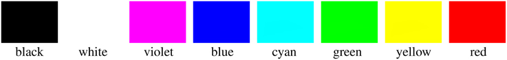
Figure 1. Selection of colors that can be applied to the background and ranges of the plotted matrix.

Intermediate color transformations are encoded in a dictionary containing 8² unique 3 element vectors, each representing red, green, and blue colors. The appropriate color transformation vector is uploaded to the GPU where the vector elements represent one mutually inclusive index of [0, 1, Z, 1-Z] with Z axis locations ∈ R ∣ 0 < Z < 1. Each location on the Z axis is subsequently colored in parallel by the GPU with the appropriate shade. Graph value colors are interpolated with two choices of ranges: [minimum, maximum] and [minimum, middle], [middle, maximum] graph value colors. Different depths of the graph can be highlighted by raising or lowering the ranges of colors.

Scrolling the mouse rotates neural fields in the direction of the mouse and the keyboard is used to move fields in various ways, cf. Figure 2.

FIGURE 2

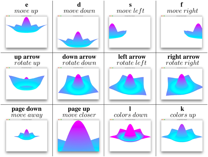
Figure 2. Keyboard keys and their corresponding movements.

Images and videos of simulations are saved, respectively in .png and .mp4 formats by using the keyboard keys in Appendix II. Visualization parameters are saved by the library after every simulation to reduce graphical adjustments during subsequent simulations of neural fields.

The show3D graphical visualization library is not limited to neural field data. Every two dimensional NumPy matrix can be displayed in 3 dimensions using the show3D library. Documentation for the show3D library's use, including a tutorial and code API, is online⁴ and packaged with example code along with the library⁵. However, there is no requirement for the library's separate download for use with the simulator because it is integrated into the Neural Field Simulator.

3. Applications

The simulator can be used to analyze spatio-temporal neural field dynamics. The simulator's open source code allows modifications and extensions to be added to the code. The subsequent sections describe few of these possible applications.

Introducing finite axonal transmission speed in neural fields substantially slows numerical computation. However, to omit finite transmission speed is to neglect biological physiology (Idiart and Abbott, 1993). Hutt and Rougier (2010) have suggested to implement finite axonal transmission speed in a computationally efficient manner that is utilized by the simulator. Numerically, the speed is infinite if $c\ge l∕\sqrt{2}\Delta t$ and there is increasing delay as c decreases.

3.1. Breather

Breather oscillations have been reported in theory (Folias and Bressloff, 2005; Hutt and Rougier, 2010) and experiments (Wang, 2010). As shown in Hutt and Rougier (2010), breathers are solutions of Equation (1) for finite axonal transmission speeds. They can be obtained and visualized in the simulator by assuming a temporally constant external input I in Equation (1). For a Gaussian-shape input with its apex at the center of the field, one overwrites the I variable section in the values.py file as

sigma = 5.65685425
I = 20*np.exp(-x**2/sigma**2)/(sigma**2*np.pi)

and change the showData variable assignment near the beginning of the values.py file to

showData = 3

to show the input I in the simulation. In the definition of I, the space variable x ∈ ${R}$² is defined to cover the spatial domain Ω (not shown in the code snippet). A field input similar to Figure 3A can be seen when the simulator is run.

FIGURE 3

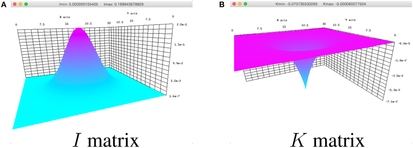
Figure 3. Breather parameters plotted in the simulator for (A) I and (B) K in Equation (1).

An inhibitory synaptic connectivity kernel, K in Equation (1), can be implemented for the breather and viewed by changing the showData and K variables in the values.py file to

showData = 4
K = -4*np.exp(-x/3)/(18*np.pi)

and running the simulator. Here, x ∈ ${R}$². An inhibitory synaptic kernel similar to the one in Figure 3B can be subsequently viewed.

After overwriting I and K as noted above, replace the following variables and function in the values.py file with the values below:

showData   = 1
endTime    = -1
dt         = 0.002
gamma      = 1.0
eta        = 0.0
c          = 500.0
l          = 30.0
n          = 512
V0         = np.zeros((n,n))
noiseVcont = np.exp(-(a**2/32.0+b**2/32.0))/
                         (np.pi*32)*0.1*np.sqrt(dt)

def updateS(V):
    return 1.0 / (1+np.exp(-10000*(V-0.005)))

Spatially localized breather oscillations are replicated by running the program. Figure 4 shows two cycles of the oscillations after setting the minimum and maximum z axis values by typing

n 0.0048 [Enter key]
y 0.0058 [Enter key]

after running the program.

FIGURE 4

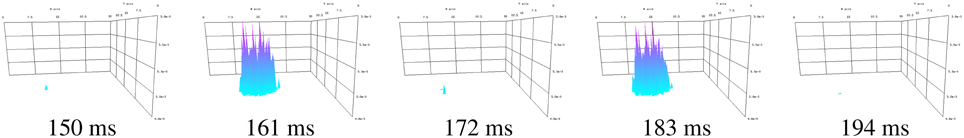
Figure 4. Two cycles of the breather oscillations.

3.2. Turing Patterns

Turing patterns (Turing, 1952) have been reported in neural field models (Atay and Hutt, 2006; Elvin et al., 2009; Steyn-Ross et al., 2010). The Neural Field Simulator is able to compute and display noisy neural field activity evolving into Turing patterns.

Static Turing patterns emerge from noisy initial conditions with the following interface properties:

showData   = 1
endTime    = 10
dt         = 0.01
gamma      = 1.0
eta        = 0.0
c          = 6364.0
l          = 90.0
n          = 512
V0         = np.ones((n,n))*5.4 +np.random.normal
                                    (0,0.1,(n,n))
noiseVcont = None
I          = np.zeros((n,n))
lins       = np.linspace(0, 9*np.pi, n) *-1
K          = np.zeros((n, n))
for i in range(n):
    K[:,i] = np.sin(lins[i])/150
for i in range(n):
    K[i] -= np.sin(lins[i])/200
def updateS(V):
    return 2.0 / (1+np.exp(-1.24*(V-3.0)))

With c = 6364 the effective speed is infinite for the given l and dt properties. Figure 5 shows the simulation starting with random field potential noise. A pattern begins to emerge at 1 s and evolves into a temporally constant Turing pattern after approximately 5 s.

FIGURE 5

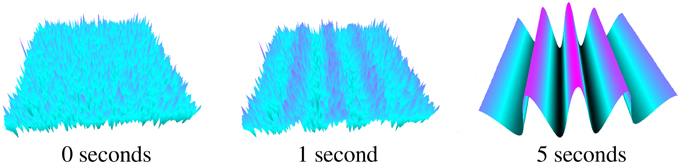
Figure 5. Static Turing pattern emerging over 5 s.

Dynamic Turing patterns emerging over time in the simulator with interface values:

showData    = 1
endTime     = 40
dt          = 0.005
gamma       = 0.82
eta         = 1.0
c           = 10.0
l           = 10.0
n           = 256
V0          = np.ones((n,n))*4.1 +np.random.normal
                                     (0,0.1,(n,n))
noiseVcont  = None
Uexcite     = np.zeros((n,n))
I           = np.ones((n,n))*2.0
lins        = np.linspace(0, 7*np.pi, n) *-1
localStrong = np.linspace(0, np.pi, n)
K           = np.zeros((n, n))
for i in range(n):
K[:,i] = np.sin(lins[i]) * np.sin(localStrong[i])
for i in range(n):
K[i] -= np.sin(lins[i]) * np.sin(localStrong[i])
def updateS(V):
    return 1.0 / (1+np.exp(-5.5*(V-3.0)))

Figure 6 shows a typical simulation, given random starting field potential noise, with different Turing patterns materializing. Activity patterns form at varying intervals, generally every few seconds, throughout the simulation. The times in Figure 6 were chosen for clear displays of different (vertical, cone, and horizontal) patterns.

FIGURE 6

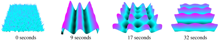
Figure 6. Turing patterns in neural field activity forming over time during the same simulation.

3.3. Finite Spreading Speed

Stimulating a neural population at a single location, as is done in typical physiological experiments applying external stimuli, the neural activity spreads in the population. Since finite transmission speed represents delayed spatial interaction in the population under study, it affects the spreading speed of activity (Hutt, 2007). If the transmission speed is infinite, the activity spreads diffusively involving the instantaneous activation at all spatial locations. Conversely, finite transmission speed delays the activity spread leading to a slowly-moving spreading front (Hutt and Atay, 2006; Hutt, 2009). Figure 7 shows numerical simulations for large (top row) and small speeds (bottom row), other parameters are identical.

FIGURE 7

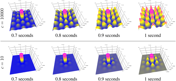
Figure 7. Activity spread with large speed c (top) and small speed c (bottom).

The simulator allows the transmission speed to be examined closely in the visualization window by decreasing the maximum z axis value to be close to the original field value. This was done in Figure 7 by typing

y 2.00002 [Enter key]

after starting the simulator and before beginning the simulation.

The parameters to achieve the results in Figure 7 are

showData   = 1
endTime    = 1
dt         = 0.004
gamma      = 1.0
eta        = 0.35
c          = 10.0
l          = 10.0
n          = 256
V0         = np.ones((n,n))*2.0
noiseVcont = None
Uexcite    = np.zeros((n,n))
I          = 2.0 *np.exp(-x**2/0.04)/(0.04*np.pi)
phi = np.pi/3
k_c = 10*np.pi/l
K   = 0.1*(np.cos(k_c*a) + \
           np.cos(k_c*(a*np.cos(phi)+b*np.
                            sin(phi))) + \
           np.cos(k_c*(a*np.cos(phi*2)+b*np.sin
                                 (phi*2)))) * \
           np.exp(-x/10.0)*(l/float(n))**2
def updateS(V):
    return 2.0 / (1+np.exp(-5.5*(V-3.0)))

where c is chosen according to the values given in Figure 7.

3.4. Extensions

The simulator, being open source, allows the tailoring of code to provide modifications and extensions. An example extension is the addition of a graphical interface to modify parameters and simulate neural fields. Figure 8 shows an example interface coded with the wxPython⁶ toolkit. Simulations are started, paused, continued, and started anew by clicking a button.

FIGURE 8

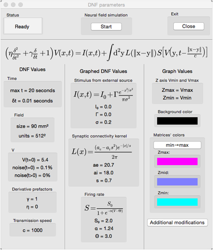
Figure 8. A graphical interface for the simulator.

Neural field parameters can be modified prior to and during simulations by clicking on the appropriate area of the interface and completing a pop-up dialogue. Running simulations are automatically paused when a mouse hovers above parameter areas of the interface. There is a symbiosis among the show3D library discussed in Section 2.3 and the parameter selection interface. It is possible to view the external input stimulus, kernel, and firing rate in the GLFW window by adding a mouse event and hovering over these sections to automatically view the respective matrices. Viewing these elements while changing their parameters can help to fine-tune field parameters. Moving the mouse away from these areas unpauses paused simulations and the field potential matrix is shown in the GLFW window. Further synergy between the interface and show3D library is implemented with the option to alter graph values from the interface where z axis limits and colors can be selected.

4. Discussion

The Neural Field Simulator and its dependencies are cross-platform. However, the simulator interacts with graphics hardware using system-specific drivers which can result in problems on some operating systems. The graphical user interface in Section 3.4 is an example of this where the cross platform wxPython toolkit uses OpenGL to draw to the screen. The show3D library likewise uses OpenGL to interact with GPU. The graphical user interface and show3D library function symbiotically on Mac systems via the Apple Graphics Library. Conversely, on other operating systems such as Linux and Windows, unfortunately the separate utilization of OpenGL causes the simulator to crash. To this end, the current version of the simulator is released without the addition of extensions in order to operate properly on every major operating system. Nevertheless, a graphical interface can be a good choice with an appropriate single operating system.

Apart from the software implementation, in future work some model assumptions can be released. The square geometry can be recast easily to a rectangular geometry, whereas more general geometries (e.g., the impressive implementation work in The Virtual Brain Sanz Leon et al., 2015) will take more numerical effort. Periodic boundary conditions guarantee the simple application of the FFT, effective implementations of other boundary conditions like Dirichlet conditions [V(z, t) = const, z ∈ ∂Ω] will demand some implementation changes in the spatial integral computation. Such modifications may still retain the fundamental implementation of the FFT. In contrast, rejecting the homogeneity hypothesis of spatial interactions, i.e., K = K(x, y) ≠ K(x − y), abolishes the convolution structure and slows down the numerical simulation, cf. Appendix I.

Future work will extend the NFM model to multiple equations to render the model even more biologically plausible. In addition, an extension of the implementation to a mixture of constant and space-dependent delays as considered by Veltz and Faugeras (2011) will be interesting.

Conflict of Interest Statement

The authors declare that the research was conducted in the absence of any commercial or financial relationships that could be construed as a potential conflict of interest.

Acknowledgments

The authors thank Kevin Green for valuable testing of the software under MacOS and Linux and for providing system parameters for Figure 6. This work is funded by the European Research Council for support under the European Union's Seventh Framework Programme (FP7/2007-2013), ERC grant agreement No. 257253 (MATHANA project).

Footnotes

1. ^https://gforge.inria.fr/projects/nfsimulator/.

2. ^http://nfsimulator.gforge.inria.fr.

3. ^https://senselab.med.yale.edu/ModelDB/showModel.cshtml?model=184479.

4. ^http://show3d.gforge.inria.fr/index.html.

5. ^https://gforge.inria.fr/projects/show3d/.

6. ^http://www.wxpython.org.

References

Atay, F. M., and Hutt, A. (2006). Neural fields with distributed transmission speeds and long-range feedback delays. SIAM J. Appl. Dyn. Syst. 5, 670–698. doi: 10.1137/050629367

CrossRef Full Text | Google Scholar

beim Graben, P., and Hutt, A. (2014). Attractor and saddle node dynamics in heterogeneous neural fields. EPJ Nonlin. Biomed. Phys. 2, 4. doi: 10.1140/epjnbp17

CrossRef Full Text | Google Scholar

Brackley, C. A., and Turner, M. (2009). Persistent fluctuations of activity in undriven continuum neural field models with power-law connections. Phys. Rev. E 79:011918. doi: 10.1103/PhysRevE.79.011918

PubMed Abstract | CrossRef Full Text | Google Scholar

Bressloff, P. (2012). Spatiotemporal dynamics of continuum neural fields. J. Phys. A 45:033001. doi: 10.1088/1751-8113/45/3/033001

CrossRef Full Text | Google Scholar

Bressloff, P. C. (2001). Traveling fronts and wave propagation failure in an inhomogeneous neural network. Phys. D 155, 83–100. doi: 10.1016/S0167-2789(01)00266-4

CrossRef Full Text | Google Scholar

Buckwar, E., Kuske, R., Mohammed, S., and Shardlow, T. (2008). Weak convergence of the euler scheme for stochastic differential delay equations. LMS J. Comput. Math. 11, 60–99. doi: 10.1112/S146115700000053X

CrossRef Full Text | Google Scholar

Buckwar, E., and Winkler, R. (2006). Multi-step methods for sdes and their application to problems with small noise. SIAM J. Num. Anal. 44, 779–803. doi: 10.1137/040602857

CrossRef Full Text | Google Scholar

Buckwar, E., and Winkler, R. (2007). Multi-step maruyama methods for stochastic delay differential equations. Stoch. Anal. Appl. 25, 933–959. doi: 10.1080/07362990701540311

CrossRef Full Text | Google Scholar

Carletti, M. (2006). Numerical solution of stochastic differential problems in the biosciences. J. Comp. Appl. Math. 185, 422–440. doi: 10.1016/j.cam.2005.03.020

CrossRef Full Text | Google Scholar

Carnevale, N., and Hines, M. (eds.). (2006). The NEURON Book. Cambridge, UK: Cambridge University Press.

Google Scholar

Coombes, S. (2005). Waves, bumps and patterns in neural field theories. Biol. Cybern. 93, 91–108. doi: 10.1007/s00422-005-0574-y

PubMed Abstract | CrossRef Full Text | Google Scholar

Coombes, S., beim Graben, P., Potthast, R., and Wright, J. (eds.). (2014). Neural Fields: Theory and Applications. New York, NY: Springer.

Google Scholar

Coombes, S., Laing, C., Schmidt, H., Svanstedt, N., and Wyller, J. (2012). Waves in random neural media. Disc. Cont. Dyn. Syst. A 32, 2951–2970. doi: 10.3934/dcds.2012.32.2951

CrossRef Full Text | Google Scholar

Coombes, S., and Owen, M. (2005). Bumps, breathers, and waves in a neural network with spike frequency adaptation. Phys. Rev. Lett. 94:148102. doi: 10.1103/PhysRevLett.94.148102

PubMed Abstract | CrossRef Full Text | Google Scholar

Coombes, S., Venkov, N., Shiau, L., Bojak, I., Liley, D., and Laing, C. (2007). Modeling electrocortical activity through improved local approximations of integral neural field equations. Phys. Rev. E 76:051901. doi: 10.1103/PhysRevE.76.051901

PubMed Abstract | CrossRef Full Text | Google Scholar

Deco, G., Jirsa, V. K., Robinson, P., Breakspear, M., and Friston, K. (2008). The dynamic brain: from spiking neurons to neural masses and cortical fields. PLoS Comput. Biol. 4:e1000092. doi: 10.1371/journal.pcbi.1000092

PubMed Abstract | CrossRef Full Text | Google Scholar

Demeulemeester, H., Vandesande, F., Orban, G., Brandon, C., and Vanderhaeghen, J. J. (1988). Heterogeneity of gabaergic cells in cat visual cortex. J. Neurosci. 8, 988–1000.

PubMed Abstract | Google Scholar

Elvin, A. J., Laing, C. R., and Roberts, M. G. (2009). Transient turing patterns in a neural field model. Phys. Rev. E 79:011911. doi: 10.1103/PhysRevE.79.011911

PubMed Abstract | CrossRef Full Text | Google Scholar

Faye, G., and Faugeras, O. (2010). Some theoretical and numerical results for delayed neural field equations. Phys. D 239, 561–578. doi: 10.1016/j.physd.2010.01.010

CrossRef Full Text | Google Scholar

Folias, S. E., and Bressloff, P. C. (2005). Breathers in two-dimensional neural media. Phys. Rev. Lett. 95:208107. doi: 10.1103/PhysRevLett.95.208107

PubMed Abstract | CrossRef Full Text | Google Scholar

Friston, K. J., Kahan, J., Biswal, B., and Razi, A. (2014). A DCM for resting state fMRI. Neuroimage 94, 396–407. doi: 10.1016/j.neuroimage.2013.12.009

PubMed Abstract | CrossRef Full Text | Google Scholar

Hashemi, M., Hutt, A., and Sleigh, J. (2014). Anesthetic action on extra-synaptic receptors: effects in neural population models of EEG activity. Front. Syst. Neurosci. 8:232. doi: 10.3389/fnsys.2014.00232

PubMed Abstract | CrossRef Full Text | Google Scholar

Hutt, A. (2007). Generalization of the reaction-diffusion, Swift-Hohenberg, and Kuramoto-Sivashinsky equations and effects of finite propagation speeds. Phys. Rev. E 75:026214. doi: 10.1103/PhysRevE.75.026214

PubMed Abstract | CrossRef Full Text | Google Scholar

Hutt, A. (2009). Oscillatory activity in excitable neural systems. Contemp. Phys. 51, 3–16. doi: 10.1080/00107510903293710

CrossRef Full Text | Google Scholar

Hutt, A., and Atay, F. (2006). Effects of distributed transmission speeds on propagating activity in neural populations. Phys. Rev. E 73:021906. doi: 10.1103/PhysRevE.73.021906

PubMed Abstract | CrossRef Full Text | Google Scholar

Hutt, A., Bestehorn, M., and Wennekers, T. (2003). Pattern formation in intracortical neuronal fields. Netw. Comput. Neural Syst. 14, 351–368. doi: 10.1088/0954-898X_14_2_310

PubMed Abstract | CrossRef Full Text | Google Scholar

Hutt, A., and Buhry, L. (2014). Study of GABAergic extra-synaptic tonic inhibition in single neurons and neural populations by traversing neural scales: application to propofol-induced anaesthesia. J. Comput. Neurosci. 37, 417–437. doi: 10.1007/s10827-014-0512-x

PubMed Abstract | CrossRef Full Text | Google Scholar

Hutt, A., and Lefebvre, J. (in press). Stochastic center manifold analysis in scalar nonlinear systems involving distributed delays and additive noise. Markov Process. Rel. Fields. Available online at: https://hal.inria.fr/hal-01006388

Hutt, A., and Rougier, N. (2014). “Numerical simulation scheme of one- and two-dimensional neural fields involving space-dependent delays,” in Neural Field Theory, eds P. beim Graben, S. Coombes, R. Potthast, and J. Wright (Berlin: Springer-Verlag), 175–183.

Google Scholar

Hutt, A., and Rougier, N. (2010). Activity spread and breathers induced by finite transmission speeds in two-dimensional neural fields. Phys. Rev. E 82:R055701. doi: 10.1103/PhysRevE.82.055701

PubMed Abstract | CrossRef Full Text | Google Scholar

Hutt, A., Sutherland, C., and Longtin, A. (2008). Driving neural oscillations with correlated spatial input and topographic feedback. Phys. Rev. E 78:021911. doi: 10.1103/PhysRevE.78.021911

PubMed Abstract | CrossRef Full Text | Google Scholar

Idiart, M. A. P., and Abbott, L. F. (1993). Propagation of excitation in neural network models. Netw. Comput. Neural Syst. 4, 285–294. doi: 10.1088/0954-898X_4_3_003

CrossRef Full Text | Google Scholar

Jirsa, V. K., and Haken, H. (1996). Field theory of electromagnetic brain activity. Phys. Rev. Lett. 77, 960–963.

PubMed Abstract | Google Scholar

Jirsa, V., Jantzen, K., Fuchs, A., and Kelso, J. (2002). Spatiotemporal forward solution of the EEG and MEG using network modelling. IEEE Trans. Med. Imag. 21, 493–504. doi: 10.1109/TMI.2002.1009385

CrossRef Full Text | Google Scholar

Kilpatrick, Z. P., and Bressloff, P. C. (2010). Binocular rivalry in a competitive neural network with synaptic depression. SIAM J. Appl. Dyn. Syst. 9, 1303–1347. doi: 10.1137/100788872

CrossRef Full Text | Google Scholar

Laing, C. (2005). Spiral waves in nonlocal equations. SIAM J. Appl. Dyn. Syst. 4, 588–606. doi: 10.1137/040612890

CrossRef Full Text | Google Scholar

Langtangen, H. P. (2006). “Numerical computing in python,” in Python Scripting for Computational Science, Volume 3 of Texts in Computational Science and Engineering, eds T. J. Barth, M. Griebel, D. E. Keyes, R. M. Nieminen, D. Roose, and T. Schlick (Berlin; Heidelberg: Springer), 131–181.

Google Scholar

Molaee-Ardekani, B., Senhadji, L., Shamsollahi, M. B., Vosoughi-Vahdat, B., and Wodey, E. (2007). Brain activity modeling in general anesthesia: enhancing local mean-field models using a slow adaptive firing rate. Phys. Rev. E 76:041911. doi: 10.1103/PhysRevE.76.041911

PubMed Abstract | CrossRef Full Text | Google Scholar

Nunez, P. (1974). The brain wave equation: a model for the EEG. Math. Biosci. 21, 279–291.

Google Scholar

Nunez, P. (2000). Toward a quantitative description of large-scale neocortical dynamic function and EEG. Behav. Brain Sci. 23, 371–437. doi: 10.1017/S0140525X00003253

PubMed Abstract | CrossRef Full Text | Google Scholar

Nunez, P., and Srinivasan, R. (2006). Electric Fields of the Brain: The Neurophysics of EEG. New York, NY; Oxford: Oxford University Press.

Google Scholar

Owen, M. R., Laing, C. R., and Coombes, S. (2007). Bumps and rings in a two-dimensional neural field: splitting and rotational instabilities. New J. Phys. 9:378. doi: 10.1088/1367-2630/9/10/378

CrossRef Full Text | Google Scholar

Pinotsis, D., and Friston, K. (2014). Extracting novel information from neuroimaging data using neural fields. EPJ Nonlin. Biomed. Phys. 2, 5. doi: 10.1140/epjnbp18

CrossRef Full Text | Google Scholar

Pinotsis, D. A., Moran, R. J, and Friston, K. J. (2012). Dynamic causal modeling with neural fields. Neuroimage 59, 1261–1274. doi: 10.1016/j.neuroimage.2011.08.020

PubMed Abstract | CrossRef Full Text | Google Scholar

Pinotsis, D. A., Schwarzkopf, D. S., Litvak, V., Rees, G., Barnes, G., and Friston, K. J. (2013). Dynamic causal modelling of lateral interactions in the visual cortex. Neuroimage 66, 563–576. doi: 10.1016/j.neuroimage.2012.10.078

PubMed Abstract | CrossRef Full Text | Google Scholar

Pinto, D., and Ermentrout, G. (2001). Spatially structured activity in synaptically coupled neuronal networks: I. travelling fronts and pulses. SIAM J. Appl. Math. 62, 206–225. doi: 10.1137/S0036139900346453

CrossRef Full Text | Google Scholar

Qubbaj, M. R., and Jirsa, V. K. (2007). Neural field dynamics with heterogeneous connection topology. Phys. Rev. Lett. 98:238102. doi: 10.1103/PhysRevLett.98.238102

PubMed Abstract | CrossRef Full Text | Google Scholar

Rosenkilde, C. (1979). Functional heterogeneity of the prefrontal cortex in the monkey: a review. Behav. Neural Biol. 25, 301–345.

PubMed Abstract | Google Scholar

Rossant, C., and Harris, K. D. (2013). Hardware-accelerated interactive data visualization for neuroscience in python. Front. Neuroinform. 7:36. doi: 10.3389/fninf.2013.00036

PubMed Abstract | CrossRef Full Text | Google Scholar

Rougier, N. P., and Fix, J. (2012). DANA: distributed numerical and adaptive modelling framework. Network 23, 237–253. doi: 10.3109/0954898X.2012.721573

PubMed Abstract | CrossRef Full Text | Google Scholar

Rougier, N., and Hutt, A. (2011). Synchronous and asynchronous evaluation of dynamic neural fields. J. Diff. Equ. Appl. 17, 1119–1133. doi: 10.1080/10236190903051575

CrossRef Full Text | Google Scholar

Sanz Leon, P., Knock, S. A., Spiegler, A., and Jirsa, V. K. (2015). Mathematical framework for large-scale brain network modeling in the virtual brain. Neuroimage 111, 385–430. doi: 10.1016/j.neuroimage.2015.01.002

PubMed Abstract | CrossRef Full Text | Google Scholar

Sanz Leon, P., Knock, S. A., Woodman, M. M., Domide, L., Mersmann, J., McIntosh, A., et al. (2013). The Virtual Brain: a simulator of primate brain network dynamics. Front. Neuroinform. 7:10. doi: 10.3389/fninf.2013.00010

PubMed Abstract | CrossRef Full Text | Google Scholar

Schmidt, H., Hutt, A., and Schimansky-Geier, L. (2009). Wave fronts in inhomogeneous neural field models. Phys. D 238, 1101–1112. doi: 10.1016/j.physd.2009.02.017

CrossRef Full Text | Google Scholar

Steyn-Ross, M. L., Steyn-Ross, D. A., Wilson, M. T., and Sleigh, J. W. (2010). “Cortical patterns and gamma genesis are modulated by reversal potentials and gap-junction diffusion,” in Modeling Phase Transitions in the Brain, Vol. 4 of Springer Series in Computational Neuroscience, eds D. A. Steyn-Ross and M. Steyn-Ross (New York, NY: Springer), 271–299.

Google Scholar

Stimberg, M., Goodman, D. F., Benichoux, V., and Brette, R. (2014). Equation-oriented specification of neural models for simulations. Front. Neuroinform. 8:6. doi: 10.3389/fninf.2014.00006

PubMed Abstract | CrossRef Full Text | Google Scholar

Turing, A. (1952). The chemical basis of morphogenesis. Philos. Trans. R. Soc. Lond. B Biol. Sci. 237, 37–72.

Google Scholar

Van Loan, C. (1991). Computational Frameworks for the Fast Fourier Transform. Philadelphia, PA: SIAM.

Google Scholar

Veltz, R., and Faugeras, O. (2011). Stability of the stationary solutions of neural field equations with propagation delays. J. Math. Neurosci. 1:1. doi: 10.1186/2190-8567-1-1

PubMed Abstract | CrossRef Full Text | Google Scholar

Veltz, R., and Faugeras, O. (2013). A center manifold result for delayed neural fields equations. SIAM J. Math. Anal. 45, 1527–1562. doi: 10.1137/110856162

CrossRef Full Text | Google Scholar

Wang, X.-J. (2010). Neurophysiological and computational principles of cortical rhythms in cognition. Physiol. Rev. 90, 1195–1268. doi: 10.1152/physrev.00035.2008

PubMed Abstract | CrossRef Full Text | Google Scholar

Wang, Y., Markram, H., Goodman, P. H., Berger, T. K., Ma, J., and Goldman-Rakic, P. S. (2006). Heterogeneity in the pyramidal network of the medial prefrontal cortex. Nat. Neurosci. 9, 534–542. doi: 10.1038/nn1670

PubMed Abstract | CrossRef Full Text | Google Scholar

Wertheimer, M., Spillmann, L., Sarris, V., and Sekuler, R. (2012). On Perceived Motion and Figural Organization. Cambridge, MA: MITPress.

Google Scholar

Wilson, H. R., and Cowan, J. (1973). A mathematical theory of the functional dynamics of cortical and thalamic nervous tissue. Kybernetik 13, 55–80.

PubMed Abstract | Google Scholar

Wright, J. J., and Kydd, R. (1992). The electroencephalogram and cortical neural networks. Network 3, 341–362. doi: 10.1088/0954-898X_3_3_006

CrossRef Full Text | Google Scholar

Wright, J. J. and Liley, D. T. J. (1994). A millimetric-scale simulation of electrocortical wave dynamics based on anatomical estimates of cortical synaptic density. Netw. Comput. Neural Syst. 5, 191–202. doi: 10.1088/0954-898X_5_2_005

CrossRef Full Text | Google Scholar

Appendix I

Heterogeneous Neural Fields

Heterogeneous neural fields have attracted increased attention in recent years (Bressloff, 2001; Qubbaj and Jirsa, 2007; Brackley and Turner, 2009; Schmidt et al., 2009; Coombes et al., 2012; beim Graben and Hutt, 2014) since they have been found in biological neural networks such as the prefrontal cortex (Rosenkilde, 1979; Wang et al., 2006) and visual cortex (Demeulemeester et al., 1988). In order to study the neural population activity in such systems, the present implementation could be extended along the following mathematical reasoning. The integral in Equation (1) may be re-written as

$\begin{array}{l}{\displaystyle {\int }_{\Omega }{\text{d}}^2}yK(x,y)S\left[V\left(y,t-\frac{\parallel x-y\parallel }{c}\right)\right]\hfill \\ ={\displaystyle {\int }_{\Omega }{\text{d}}^2}y{\displaystyle {\int }_{-\infty }^{\infty }d}\tau K(x,y)\delta (\tau -t+\frac{\parallel x-y\parallel }{c})S\left[V\left(y,\tau \right)\right]\hfill \\ ={\displaystyle {\int }_{\Omega }{\text{d}}^2}y{\displaystyle {\int }_0^{{\tau }_{max}}d}TD(x-y,T)R(x,y,t-T)\hfill \end{array}$

with D(x, t) = δ(∥ x ∥ ∕c − t), R(x, y, t) = K(x, y)S[V(y, t)]. This integral still has a spatial convolution structure; however, it is not perfect since R includes the spatial location x. The numerical simulation of the integral consequently involves $n^4{n}_{rings}$ summands and the numerical implementation is slower than in the homogeneous case. The formulation of heterogeneous neural fields is not implemented yet, but it will be part of a future update.

Appendix II

TABLE A1

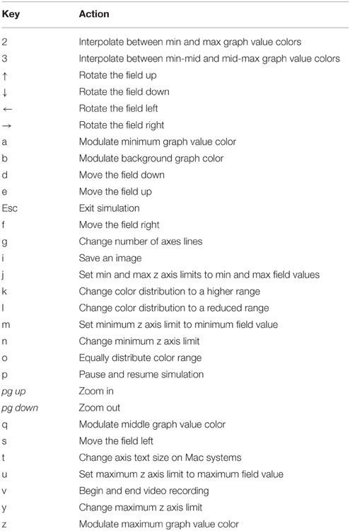
Table A1. Keyboard keys and their actions.