 Robert LeBourdais
 Gabrielle N. Grifno
 Rohin Banerji
 Kathryn Regan
 Bela Suki
 Hadi T. Nia
- Department of Biomedical Engineering, Boston University, Boston, MA, United States
Lung diseases such as cancer substantially alter the mechanical properties of the organ with direct impact on the development, progression, diagnosis, and treatment response of diseases. Despite significant interest in the lung’s material properties, measuring the stiffness of intact lungs at sub-alveolar resolution has not been possible. Recently, we developed the crystal ribcage to image functioning lungs at optical resolution while controlling physiological parameters such as air pressure. Here, we introduce a data-driven, multiscale network model that takes images of the lung at different distending pressures, acquired via the crystal ribcage, and produces corresponding absolute stiffness maps. Following validation, we report absolute stiffness maps of the functioning lung at microscale resolution in health and disease. For representative images of a healthy lung and a lung with primary cancer, we find that while the lung exhibits significant stiffness heterogeneity at the microscale, primary tumors introduce even greater heterogeneity into the lung’s microenvironment. Additionally, we observe that while the healthy alveoli exhibit strain-stiffening of ∼1.75 times, the tumor’s stiffness increases by a factor of six across the range of measured transpulmonary pressures. While the tumor stiffness is 1.4 times the lung stiffness at a transpulmonary pressure of three cmH2O, the tumor’s mean stiffness is nearly five times greater than that of the surrounding tissue at a transpulmonary pressure of 18 cmH2O. Finally, we report that the variance in both strain and stiffness increases with transpulmonary pressure in both the healthy and cancerous lungs. Our new method allows quantitative assessment of disease-induced stiffness changes in the alveoli with implications for mechanotransduction.
1 Introduction
Altered stiffness is one of the four physical hallmarks of cancer (Nia et al., 2020a; Zhang et al., 2023a), with implications for the development, progression, diagnosis, and treatment response of solid cancers. Biologically, elevated stiffness promotes proliferation (Ulrich et al., 2009), invasiveness (Tse et al., 2012), and metastasis (Wirtz et al., 2011) through activation of mechanosensitive signaling pathways; clinically, an increase in stiffness is associated with an increased risk of breast cancer (Boyd et al., 2014) and mortality (Evans et al., 2012). In diagnostics, cellular and extracellular stiffness are traditional markers of cancer (Cochlin et al., 2002; Goenezen et al., 2012) and are predictive of a tumor’s stage (Panzetta et al., 2017). In therapy, increased stiffness is linked to reduced efficiency of drug delivery (Nia et al., 2019). Furthermore, determining the stiffness of the tumors and their surrounding tissue is an essential precursor for estimating solid mechanical stresses, another physical hallmark of cancer (Nia et al., 2016; Nia et al., 2018; Nia et al., 2019; Nia et al., 2020b; Zhang et al., 2023a; Zhang et al., 2023b). Despite this, the lung’s or a lung tumor’s stiffness has not been reported under the following conditions: (i) across a range of physiologically relevant pressures, (ii) noninvasively, i.e., without sectioning of the tissue, (iii) under realistic boundary conditions, and (iv) at microscale resolution.
Although elastography encompasses a broad range of techniques for assessing the material properties of biological tissues, each method presents limitations when addressing our specific problem (Costa, 2004; De et al., 2010; Evans et al., 2012; Goenezen et al., 2012; Kennedy et al., 2014; Garra, 2015; Schregel et al., 2018; Seidl et al., 2020; Silva et al., 2020; Ghiuchici et al., 2021; Kuo et al., 2021; Wang et al., 2023). The gold-standard method for microscale elastography is atomic-force microscopy (Krieg et al., 2018), which boasts extremely high-resolution, absolute measurements of stiffness. However, tissue preparation for AFM involves resection and submersion in saline, which disrupts the mechanical integrity of the sample and the alveolar air-liquid interface (Liu and Tschumperlin, 2011). Though CT and MRI elastography preserve the mechanical environment of the organ, these methods have poor spatiotemporal resolution, and they typically report strain rather than absolute stiffness (Barbone and Bamber, 2002; Barbone and Gokhale, 2004). Although strain elastography based on modalities like synchrotron microCT (Cercos-Pita et al., 2022) have near-micron spatial resolution, to our knowledge, these methods lack the control and temporal resolution needed for tracking the same region of interest at alveolar resolution across changes in inflation pressure. Optical elastography (Kennedy et al., 2014; Kennedy et al., 2017; Wang et al., 2023) offers an alternative method for more precisely estimating the displacements throughout a biological sample. For example, recent papers have implemented optical elastography based on digital image correlation (DIC) to quantify the lung’s strain (Nelson et al., 2023) and stiffness (Maghsoudi-Ganjeh et al., 2021); but in each case, the empirical method does not provide physiologically realistic boundary conditions, and the measurements are not at alveolar resolution. Using optical elastography based on deformable image registration, our group recently mapped the elasticity of resected biological samples at optical resolution either by embedding them in thermo-responsive hydrogels (Regan et al., 2023) or by adhering precision-cut lung slices (Kim et al., 2023). However, these methods also involve resection of the organ and embedding the sample in saline, which does not preserve the organ’s boundary conditions and disrupts the air-liquid interface in the lung.
With that goal in mind, we recently developed the crystal ribcage (Banerji et al., 2023), which preserves the integrity of the organ and emulates the in vivo boundary conditions seen by the lung, while at the same time enabling real-time microscopy of the entire surface during dynamic ventilation at cellular resolution (Supplementary Figure S1). Unlike intravital imaging methods (Looney et al., 2011; Looney and Bhattacharya, 2014; Entenberg et al., 2018) wherein the lung is immobilized by vacuum or glue, and which thus compromise the breathing mechanics of the lung at the imaging site, the plasma-treated crystal ribcage provides a lubricious, geometrically realistic boundary condition, allowing mechanical characterization of the lung throughout the breathing cycle in health and disease. While the tissue preparation involves resection of the organ from the mouse’s thorax, the ex vivo lung, with its pleura intact, is imaged immediately after resection, and the lung can be vascularly perfused with complete media to maintain cell health throughout the course of imaging. Consequently, our platform preserves the in vivo physiological conditions of the lung. By developing an optical elastography platform based on the crystal ribcage apparatus, we can assess the mechanical properties of the ex vivo lung in health and disease with high spatiotemporal resolution and with physiologically realistic boundary conditions.
Here, to accurately estimate the in vivo mechanical properties of the lung in health and disease, we adopt a multiscale-modeling approach that couples the microscale displacements estimated through deformable image registration and the mean, strain-dependent stiffnesses estimated using a nonlinear, finite-element model of the lung. We validate the multiscale model against a virtual, finite-element model of the lung with a cancerous tumor, demonstrating that the method is capable of accurately recovering the mechanical properties throughout the domain even in the presence of pathology. Upon applying the model to images of the lung within the crystal ribcage, we find that (i) the stiffness of the lung tissue increases nonlinearly with transpulmonary pressure across the full range of end-expiratory to end-inspiratory pressures; (ii) there is significant heterogeneity in material properties at alveolar resolution; (iii) the intratumor stiffness increasingly exceeds the extratumor stiffness across the entire range of pressures; and finally, (iv) the variance in stiffness increases with strain for both the healthy and cancerous tissue. While the present study characterizes the micromechanics of the healthy lung and the lung with cancerous tumors, the method has the potential to be applied to a wide range of disease states such as fibrosis, COPD, and respiratory infections.
2 Methods
2.1 Mouse model of lung cancer, crystal ribcage fabrication, and imaging
2.1.1 Animal use ethics
All experiments conformed to the ethical principles and guidelines under protocols set forth and approved by the Boston University Institutional Animal Care and Use Committee (protocol number PROTO201900086). All animal procedures were compliant with ARRIVE guidelines. Mice were housed in ambient temperature and humidity and 12-h light–dark conditions under pathogen-free conditions at the Boston University Animal Science Center. No housing or handling exceptions were made for this study.
2.1.2 Mice
We used 11- to 23-week-old male and female mice for experimental procedures including healthy lung imaging and generating models of primary cancer, as previously described (Banerji et al., 2023). A breeding pair of transgenic B6.129(Cg)-Gt (ROSA)26Sortm4 (ACTB-tdTomato,-EGFP)Luo/J mice (JAX, 007676, Jackson Labs) (Muzumdar et al., 2007), referred to by the abbreviation “mTmG”, was initially purchased to breed a colony; that colony was the source of all animals for healthy lung and primary cancer experiments. For the present study, which examines two representative mice from this colony, the healthy mouse was 11 weeks old at the time of imaging. The urethane mouse, serving as our model of primary cancer, was 23 weeks at the start of urethane dosing and 54 weeks at the time of imaging. Between these ages, the murine lung’s volume does not change appreciably both in our experience and per development studies (Schulte et al., 2019).
2.1.3 Primary cancer model
We adapted a previously described protocol (Janker et al., 2018; Sozio et al., 2021) to induce primary lung cancer in mTmG mouse lungs using urethane (Sigma U2500). A stock solution of urethane was prepared at a working concentration of 200 mg/mL in PBS. Mice were dosed with the urethane solution at 1 mg/g body weight, twice weekly for 5 weeks by intraperitoneal (IP) injection. Mice were sacrificed and lungs harvested for imaging in the crystal ribcage after 6–12 months. The maximum tumor size permitted for the study was 1.5 mm in diameter. Mice were excluded from the study after presenting with labored breathing, hunched posture, or ruffled fur due to tumor progression.
2.1.4 Crystal ribcage fabrication
The full development of the crystal ribcage platform is described in our previous work (Banerji et al., 2023). Briefly, microCT scans of C57BL/6 mouse chest cavity (courtesy the Hoffman group at the University of Iowa (Thiesse et al., 2010; Vasilescu et al., 2012; Kizhakke Puliyakote et al., 2016)) were segmented and refined to create the native ribcage geometry. In successive additive manufacturing and fabrication steps the ribcage model was converted into the crystal ribcage mold that was thermoformed over to create the polystyrene crystal ribcage. The internal surface was engineered to be hydrophilic to allow the lung to glide over its surface, as in the native ribcage. A six degree of freedom arm was included to rotate the crystal ribcage about any axis to image across the entire the distal lung surface using either a top-down or bottom-up configured microscope. Because lung volume changes significantly with age (Schulte et al., 2019), we have fabricated different, age-specific crystal ribcages to accommodate lungs of different sizes (Banerji et al., 2023).
2.1.5 Lung preparation
Isolated mouse lungs were ventilated and perfused as previously described (Vanderpool and Chesler, 2011; Banerji et al., 2023). Briefly, the mouse trachea was cannulated and the lungs dynamically ventilated (Kent Physiosuite Mouse Ventilator, Kent Scientific). The lungs were perfused by cannulating the pulmonary artery and left atrium, and perfusing serum-free RPMI cell culture medium (Corning) through the lung vasculature. After cannulating the trachea and mouse heart, the lung–heart bloc, was excised and placed into the crystal ribcage for ex vivo microscopy under variable quasi-static positive air pressures.
2.1.6 Lung microscopy
As previously described (Banerji et al., 2023), ex vivo lungs, under quasi-static inflation conditions and within the crystal ribcage, were imaged using (i) an upright Nikon stereomicroscope with a 1x objective, and (ii) an upright Nikon CSU-X1 spinning-disk confocal microscope with 1x, 2x, 4x and 10x objectives, using NIS-Elements acquisition software and with the environmental temperature control set to 37°C.
Z-stacks of the diseased and healthy lungs were acquired on the confocal microscope using a 561 nm laser at 20–50 ms exposure (50–20 frames per second) per frame. Voxel sizes varied based on objective used, with XY resolution varying from 1–10 μm and Z step sizes varying from 2.5–12.5 μm. Total Z-stack acquisition time was on the order of 6–15 s for each positive-end expiratory pressure (PEEP) condition.
Before imaging, lungs were gradually recruited by slowly raising the intratracheal pressure to 18 cmH2O, measured using custom sensors sensitive to 0.1 cmH2O, using a water column. The pressure was then reduced in decrements of 1 cmH2O down to 2 cmH2O. To allow the lung to relax to its steady-state condition, each pressure was maintained for 1 min before imaging.
2.2 Organ-scale geometry modeling
Figure 1 summarizes the multiscale model. In short, we (i) segment microCT images of the lung in MATLAB 2022b (The MathWorks, Inc.), (ii) construct a geometric model from the segmentation in SolidWorks 2021 (Dassault Systèmes), (iii) simulate ventilation of the organ-scale model in Abaqus 2022 (Dassault Systèmes) for a range of material coefficients, (iv) determine the coefficients that optimally reproduce the observed pressure-distension behavior of the lung in the crystal ribcage, (v) solve the inverse elasticity problem for the distribution of material properties throughout the microscale domain in arbitrary units, and finally, (vi) rescale these relative stiffnesses so that the mean value matches the stiffness of the organ-scale model, yielding our goal of recovering the absolute stiffnesses throughout the microscale domain. Given a three-dimensional microCT image (Thiesse et al., 2010; Vasilescu et al., 2012; Kizhakke Puliyakote et al., 2016) of the mouse thorax, we first construct three-dimensional geometric models (Figure 1A) of the mouse lung and ribcage for finite-element analysis as follows.
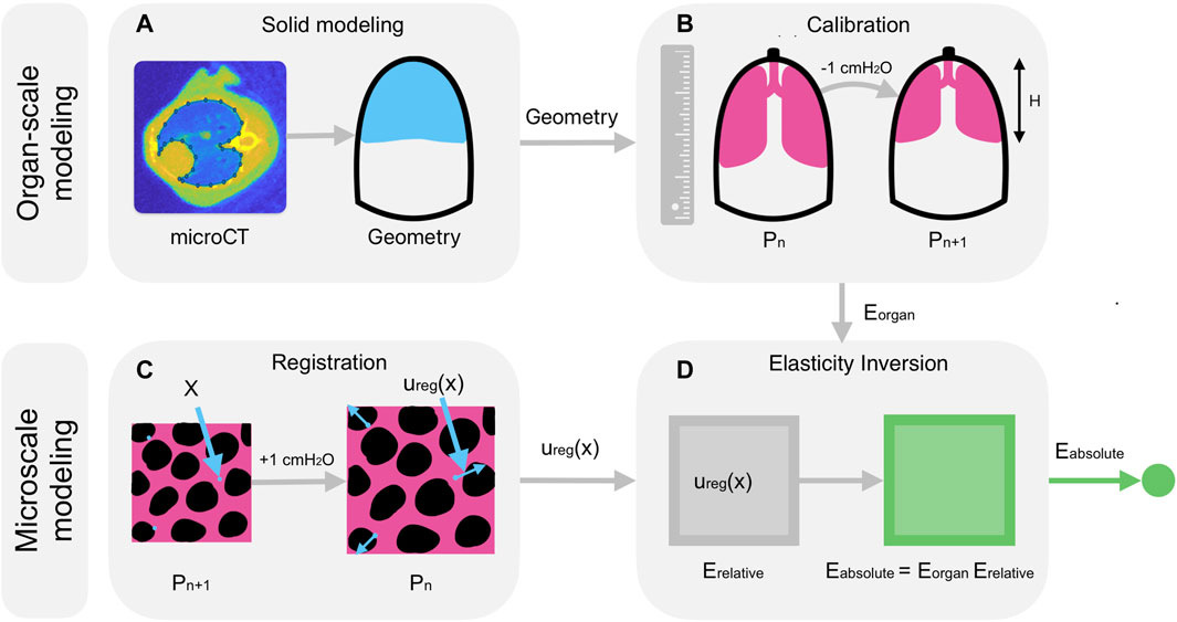
Figure 1. Model description. (A) A Bayesian classifier segments the geometries of the lung and of the ribcage from microCT images (Thiesse et al., 2010; Vasilescu et al., 2012; Kizhakke Puliyakote et al., 2016) of the mouse thorax, and the segmentation is then used to construct a solid geometry in SolidWorks for finite-element analysis. (B) After recruitment, the height,
2.2.1 Segmenting the lung and ribcage
Due to significant variations in the lung’s intensity within a microCT volume, segmenting the organ by thresholding is unreliable. To segment the lung, we thus construct a naïve, Bayesian classifier—trained on a single, two-dimensional slice of the image along with its ground-truth class labels—to differentiate the lung class
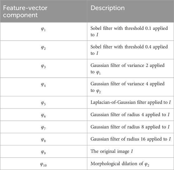
Table 1. Components of the feature vectors extracted from the microCT volume for building the Bayesian classifier. Each feature vector has ten components, each corresponding to a different transformation of the image volume. To normalize the components, each component is divided by its standard deviation.
Let
The lung segmentation
In contrast, because the intensity of bone tissue is much higher than that of other biological materials, the approach to segmenting the ribcage is simpler. Here, the ribcage segmentation
2.2.2 Constructing solid models of the lung and ribcage
From the lung segmentation
Next, to construct a point-cloud approximation of the ribcage, we first find the geometric centroid of the lung,
For each slice of the volume, we then project rays from the projection of the centroid,
In this equation,
From these point clouds, we finally construct STEP (Standard for the Exchange of Product model data defined by ISO 10303 (Pratt, 2001)) representations of the diaphragm and the ribcage using the ScanTo3D feature in SolidWorks. By cutting the ribcage surface with the diaphragm surface, and filling the space enclosed between them, we recover a simplified model of the lung that is everywhere tangent to the ribcage. This approach guarantees a priori that, at the start of each simulation, the lung geometry and the ribcage geometry are in perfect contact, preventing errors in predicted strains and stresses that may arise due to mismatch between these geometries. The STEP representations of the ribcage and the lung are then exported from SolidWorks.
2.3 Organ-scale finite-element modeling
2.3.1 Simulating the healthy lung
To perform finite-element simulations of the organ, these STEP geometries are now imported into Abaqus 2022 (Dassault Systèmes). The ribcage is taken to be a discrete, rigid part and is meshed with rigid, triangular elements. The lung is taken to be a deformable part and is meshed with C3D10 quadratic tetrahedral elements, which are chosen over C3D4 linear tetrahedral elements for their tendency to converge more quickly with coarser mesh resolutions. In simulations of the healthy lung, the lung mesh consists of 34,541 nodes and 21,945 elements; the ribcage mesh consists of 64,093 nodes and 127,697 elements. The simulation was performed on the Boston University Shared Computing Cluster hosted by the Massachusetts Green High-Performance Computing Center distributing the load over 12 processors with 4 GB of RAM per processor, each simulation completed within 7 h.
Based on prior studies and on the lung’s microstructure and constitutive behavior—which resembles a hyperelastic, tetrakaidekahedral foam whose walls are comprised of elastin, type-I collagen, and type-III collagen—the lung is modeled using the Ogden-Hill model (Berezvai and Kossa, 2017) of a hyperelastic foam (Vawter et al., 1979; Andrikakou et al., 2016). The general form of the strain-energy density function is thus taken to be
where
This strain-energy density function, and consequently the pressure, is linear in the parameter
The boundary conditions (Supplementary Figure S2) include immobilization of the ribcage, frictionless sliding contact between the lung’s upper surface and the ribcage, and negative pressure on the boundary of the lung. Although experiments involve positive-pressure ventilation, the simulation involves applying negative pressure to the external surface of the lung; the explanation for this apparent discrepancy is that the governing equations are symmetric under mutual inversion of the pressure’s sign and the surface normal’s direction, implying that the model is equally applicable to either mode of ventilation (Shi et al., 2022). Since the parts have been designed a priori to be tangent everywhere, initial contact between the surfaces is easy to establish.
While previous studies (Tawhai et al., 2009; Shi et al., 2022) have shown that gravity significantly influences the mechanics of the human lung, our model neglects the influence of gravity due to its smaller role in the mouse. Consider the conservation of linear momentum under conditions of static equilibrium, which has been rendered dimensionless (Munson et al., 2012) by factoring out the lung density
Here,
Finally, it is important to note that the lung exhibits hysteresis, with its inflation characterized by one strain-energy density function and its deflation characterized by another (Vawter et al., 1979). In this study, we elect to model the lung’s behavior during quasistatic deflation, so that our measurements used to calibrate the model are taken from states of higher pressure to states of lower pressure in near-equilibrium. The same approach can easily be repeated to recover a model of the lung’s behavior during inflation.
2.3.2 Simulating the cancerous lung
To simulate the cancerous lung, the same process is repeated, but rather than being constant, the material field
where
The ribcage mesh is the same as before, while the lung mesh now consists of 12,679 nodes and 7,766 elements. Adaptive mesh refinement, which was necessary for convergence in the neighborhood of the tumor, yielded a mesh with fewer elements relative to the simulation of the healthy lung. The simulation was performed on the Boston University Shared Computing Cluster hosted by the Massachusetts Green High-Performance Computing Center; distributing the load over 12 processors with 4 GB of RAM per processor, the simulation completed within 4 h.
2.3.3 Calibrating the organ-scale finite-element model
The finite-element simulation is repeated for different material parameters within a neighborhood of the values yielding optimal agreement between empirical and in silico outcomes. When the strain-energy density function is restricted to a single term, the parameter
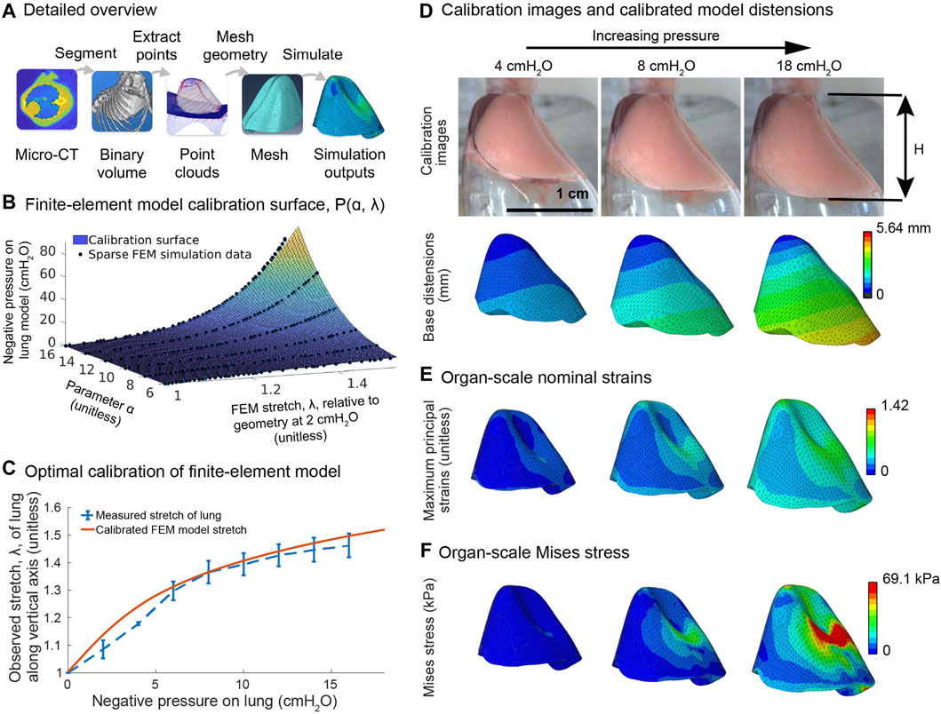
Figure 2. Constructing the finite-element model of the lung from a microCT volume and organ-scale pressure-distension data. (A) A Bayesian classifier segments the mouse lung and ribcage from a microCT volume (Thiesse et al., 2010; Vasilescu et al., 2012; Kizhakke Puliyakote et al., 2016) of the mouse thorax. From the segmentations, we construct smooth point clouds approximating the interior surfaces of the ribcage and of the diaphragm. From these point clouds, we construct solid models in SolidWorks and then mesh those models in Abaqus. (B) Pressure versus vertical stretch, λ, is recorded for simulations across a range of values for the material parameter
Based on these initial estimates, we perform simulations for
This optimization procedure is not computationally intensive; running on a personal laptop with 16 GB of RAM and a typical CPU, for example, the process completes within seconds. The outcome is a single, point estimate of the coefficients that characterize the organ-scale behavior. It should be noted that, because the model is linear in the parameter
This implies that, rather than sampling the function
2.4 Inverse elasticity problem at the microscale
2.4.1 Measuring the displacements using image registration
To measure the displacements caused by a change in distending pressure applied to the lung at cellular resolution, we leverage deformable image registration (Heinrich et al., 2012a) (Figure 1C). To prepare the images for registration, we perform an optimization to autonomously correct the bulk rotation of the material due to the natural curvature of the crystal ribcage away from the imaging plane. Because the image-registration algorithm does not, in practice, yield good estimates for the displacements along the shallow depth axis, we project the rotationally corrected images along this axis.
After preprocessing the images, we invoke the image-registration algorithm. This algorithm, which has been adapted from earlier literature (Heinrich et al., 2012a), formulates the inverse-elasticity problem as an inference problem on a Markov Random Field (MRF) to automatically determine the displacements necessary to match images of the lung at two different pressures. The observable variables of the Markov Random Field are modality-independent neighborhood descriptors (MIND) extracted from the image (Heinrich et al., 2012b), while the latent variables are the displacements necessary to minimize the sum of squared differences in these descriptors across the two images; edges between the latent variables of neighboring observables represent the constraint that displacements vary smoothly throughout the domain. Let
where the sum is taken over the points in the image domain,
2.4.2 Solving for the shear modulus parameter
To determine the relative stiffnesses of the material throughout the image domain, we leverage a Python implementation of the Adjoint-Weighted Equation (AWE) formulation of the inverse-elasticity problem (Barbone et al., 2010). Let
From the deformation gradient, we next determine the Cauchy-Green strain tensor field,
By the spectral theorem and the manifest symmetry of
The areal strain, which is a scalar field representing the fractional change in the material’s area relative to its value in the reference configuration, is then given by
The whole organ’s stress-strain behavior is well-described by a hyperelastic material law, where the nominal stress is the derivative of the strain-energy function with respect to the principal nominal stretches. If we assume that this model holds at all length scales, down to the cellular scale and for both healthy and diseased tissue, then we can use this same constitutive model when solving the inverse problem. Therefore, from the same strain-energy function introduced earlier, we recover the principal components of the first Piola-Kirchhoff stress tensor as follows.
where
For a hyperelastic material, it is well-known that the eigenvectors of the stress are aligned with the eigenvectors of the strain. Therefore, if
We can simplify the above expression by defining the tensor
Here,
From our earlier simplified form for
In the AWE formulation of the inverse elasticity problem for a linearly elastic material, we seek a variational solution for
From Holzapfel’s equation (6.180) (Holzapfel, 2000), which is reproduced below as Eq. 19, along with the strain-energy function mentioned earlier, we determine the components of the elasticity tensor,
Finally, we perform an iterative optimization to determine the Young’s modulus and Poisson’s ratio fields that optimally approximate the components this tensor. This Young’s modulus is what we ultimately report as the lung’s stiffness (Figure 1D).
2.5 Statistical comparison of intergroup and intragroup strains and stiffnesses
To characterize changes in strain and stress fields with pressure, we discretized the domain by coherence length into 50 × 50 pixel patches (See Supplementary Figure S5), the dimensions of which were chosen to minimize the correlation between image patches. We then computed the mean within each patch, along with the standard deviation across patches within the same domain. With these means and standard deviations, p-values were computed (i) across image patches within the same field in order to examine the significance of spatial variations in strain and stiffness and (ii) across pressures within the same patch in order to examine the significance of pressure-driven changes in strain and stiffness within a given patch.
3 Results and discussion
3.1 Validating the finite-element model
We begin by describing and assessing the finite-element model of the organ, which constitutes the first stage of the system. The image classifiers described in the methods yield high-quality segmentations of the lung and the ribcage. These segmentations are subsequently used to construct a realistic, though simplified, model of the lung within the crystal ribcage (Figure 2A). We find that the pressure-stretch curve of the finite-element model changes smoothly with the parameter
3.2 Validating the multiscale model
After constructing the finite-element model and calibrating its material constants, we proceed to evaluate the system’s predictive performance. To do so, we modify the calibrated finite-element model to contain a stiffer inclusion representing a tumor (Figure 3A). From the displacements of this model over a range of pressures, we solve the inverse elasticity problem in the vicinity of the tumor. Across the entire range of distending pressures, we find that the total areal strain (Figure 3B) is highly correlated with the ground-truth stiffness (Figure 3C). We further find that the stiffness estimate produced by our multiscale model (Figure 3D) is well-correlated with the ground truth. Although the prediction is somewhat biased relative to the ground truth, we find that the mean of the predicted stiffness is strongly correlated with the mean of the ground truth both inside and outside the tumor (Figure 3E). In a simpler setting, our preliminary work also indicates that the nonlinear formulation of the inverse elasticity problem accurately predicts the stiffness distribution throughout a 2D, hyperelastic membrane (Supplementary Figure S4). In contrast, our preliminary work also indicates that a piecewise-linear formulation of the inverse elasticity problem fails to do so (Supplementary Figure S5).
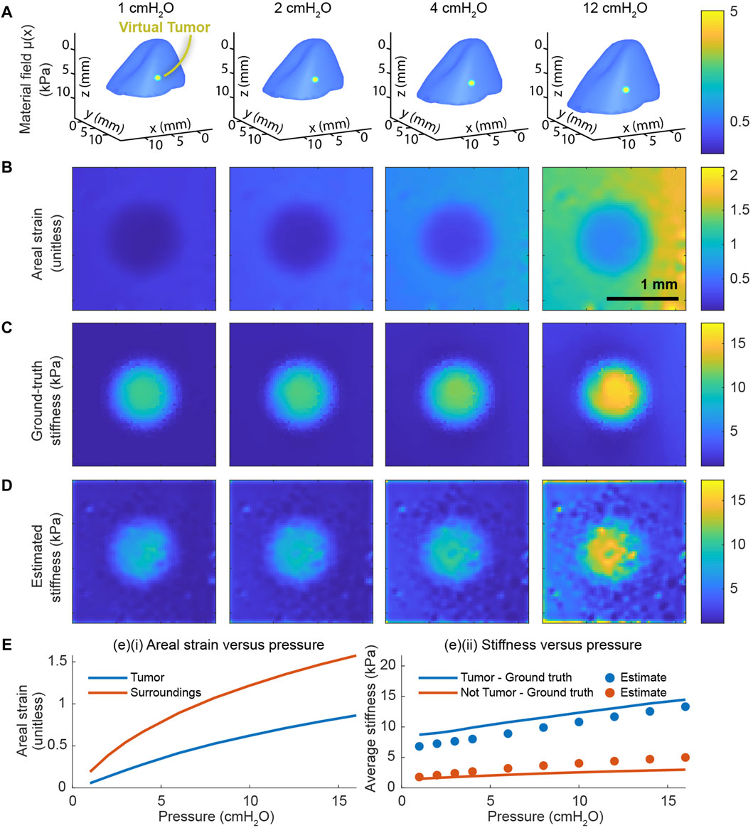
Figure 3. End-to-end validation of the whole-organ and microscale models. The validation includes applying the multiscale model to a finite-element model whose material field contains an inclusion representing a cancerous tumor. (A) The material field superposed over the deformed geometry of the finite-element model across a range of distending pressures. (B) The total areal strain at a subset of these same pressures. (C) The ground-truth stiffness distribution throughout the finite-element model determined from material field, the hyperelastic constitutive equation, and the state of deformation. (D) The corresponding stiffnesses in absolute units (kPa) throughout the domain determined by our model based on the simulated displacements. (E) The cumulative areal strain and the absolute stiffness change nonlinearly with the distending pressure. (E) (i) The average, nominal areal strain inside the tumor is consistently lower than the same outside the tumor. (E) (ii) The mean value of the ground-truth stiffness distribution is strongly correlated with the stiffness distribution predicted by the multiscale model.
3.3 Lung stiffness at alveolar resolution
After validating the model, we next apply the model to real images of the lung in the crystal ribcage to measure the stiffness of the lung in absolute units and at alveolar resolution. First, we apply the model to images of the same region of interest in the healthy lung over a range of distending pressures (Figure 4A). To demonstrate the accuracy of the registration, we warp them back to the reference configuration at 2 cmH2O (Figure 4B). We observe that the areal strain varies substantially on the length scale of an individual alveolus, with airspaces stretching much more than the septum (Figure 4C). Likewise, we see that the stiffness varies on a similar length scale, and we report for the first time, a noninvasive measurement of the absolute stiffness of the lung’s surface both in the airspace and in the septum; stiffnesses within the airspace are close to 1–2 kPa, while stiffnesses in the septum commonly reach as high as 15 kPa at higher pressures (Figure 4D). These values are consistent with measurements taken using other techniques like atomic-force microscopy (AFM), for which estimates for the lung’s shear modulus commonly range from 0.5 to 3 kPa (Polio et al., 2018; Jorba et al., 2019). Another study (Perlman and Wu, 2014) predicted that the Young’s modulus of the septum ranges from 12 kPa at low transpulmonary pressures to 140 kPa at high transpulmonary pressures; the lower bound is very close to our estimate, while the upper bound is of the same magnitude as ours (Figure 4D). Perhaps most significantly, we observe that the pattern of stiffnesses throughout the domain is conserved across the entire range of pressures. Finally, we note that the mean stiffness of the tissue rises linearly up to 7 cmH2O, and then the stiffness quickly plateaus with increasing transpulmonary pressure (Figures 4E, F). Based on the scheme previously described in the methods (Supplementary Figure S6), p-values computed using Student’s t-test indicate that the change in strain across pressures is statistically significant with p < 0.05 from 5-7 cmH2O, 7–12 cmH2O, and 12–18 cmH2O (Figure 4F). On the other hand, the change in stiffness is only statistically significant at lower pressures, owing to higher variance in the stiffness and its apparent plateau at higher pressures (Figures 4E, F). We also predict that the variance in the lung’s stiffness increases with distension (Figure 4F); this prediction is consistent with our previous, independent measurement of the lung’s strain-stiffening behavior from manual measurements of alveolar areas across different pressures (Banerji et al., 2023). To our knowledge, this is the first time that the lung’s stiffness, and its change with distension, has been measured under ex vivo conditions with physiologically realistic boundary conditions in absolute units and at alveolar resolution.
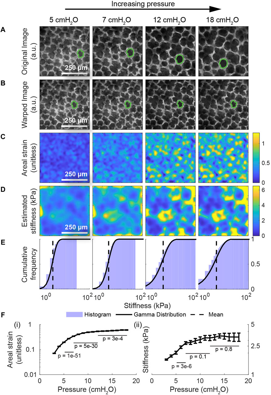
Figure 4. Providing the alveolus-scale stiffness map during the full breathing cycle in the healthy lung. (A) The same region of interest within a healthy lung from a transgenic, mTmG mouse expressing the tdTomato fluorescent label at four different distending pressures. (B) The result of computationally deforming these images back to the lung’s geometry at 2 cmH2O using the registered displacements. The displacement maps used to deform these images were subsequently used as inputs to the multiscale model to determine the distribution of stiffnesses throughout the healthy tissue. (C) The areal strain relative to the geometry at 2 cmH2O. We observe that the qualitative pattern in the computed strains is largely conserved across all pressures. Row (D) depicts the corresponding stiffnesses in absolute units throughout the domain determined by applying our model to these images. As with the areal strain maps, the stiffness maps are qualitatively similar across the whole range of pressures. (E) The histogram and corresponding Gamma distribution of the stiffnesses throughout the domain, demonstrating that the mean and the heterogeneity in the lung’s stiffness increase with distension. (F) The nonlinear change in mean strain and mean stiffness with the distending pressure. The error bars represent the standard error from the mean, computed by discretizing the domain into a coherence length of 50 × 50 pixel patches (See Supplementary Figure S6). Computed using Student’s t-test, p-values are shown for the change in strain (and for the change in stiffness) from 5-7 cmH2O, 7–12 cmH2O, and 12–18 cmH2O; the strains are consistently statistically significant, while the stiffnesses are begin statistically significant and then decrease in significance. We further observe that the variance in the stiffness increases with transpulmonary pressure, which is consistent with our previous finding on relative stiffness (Banerji et al., 2023).
Having applied the model to the healthy lung, we do the same for images of the lung with cancer (Figure 5A) to characterize the effect of cancer on the lung’s material properties. As with the previous figure, the second row (Figure 5B) shows the result of deforming these images back to the geometry of the lung at 2 cmH2O using the registered displacements. Here, we observe that the strain inside the tumor is substantially lower than the strain outside the tumor across all measured pressures (Figure 5C). Consistent with these observations, the estimated stiffness inside the tumor is substantially higher than the stiffness outside at lower pressures (Figure 5D). Whereas the majority of stiffnesses in the healthy lung are below 5 kPa at pressures up to 10 cmH2O, a large fraction of the tumor exceeds these stiffnesses at these same pressures (Figure 5F). Using the method described previously (Supplementary Figure S6), p-values computed using Student’s t-test indicate that the change in strain across pressures within the lung tissue is statistically significant with p < 0.05 from 5-7 cmH2O, 7–12 cmH2O, and 12–18 cmH2O, while changes in the strain within the tumor are insignificant at 7–12 cmH2O and 12–18 cmH2O (Figure 5F). Once again, in both types of tissue, the change in stiffness becomes insignificant at higher pressures. On the other hand, at the same pressure, the difference in strain and stiffness across groups (i.e., lung or tumor) is statistically significant with p < 0.05 across all pressures.
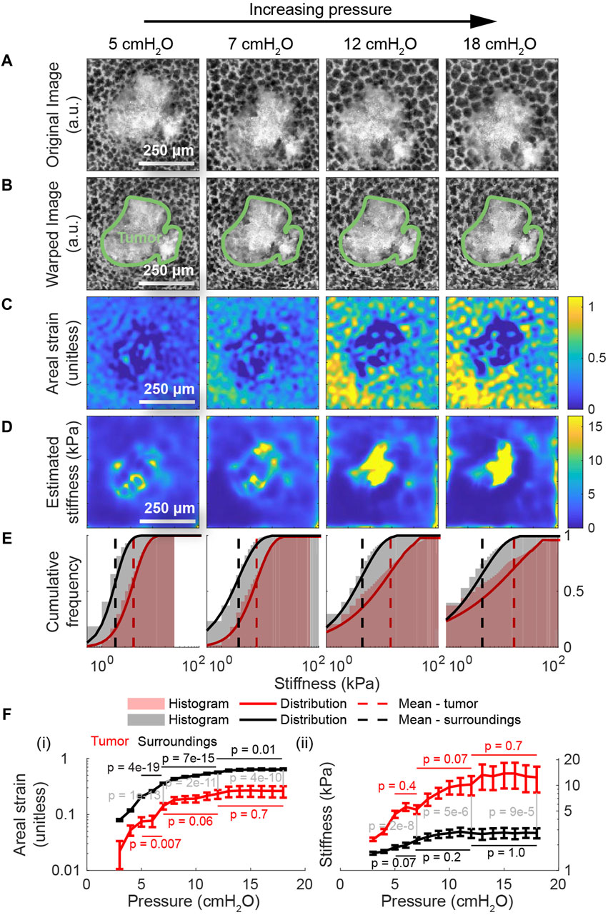
Figure 5. Applying the model to the lung with cancer. (A) The same region of interest within a lung presenting with primary cancer from a transgenic, mTmG mouse expressing the tdTomato fluorescent label at four different distending pressures. These images were used as inputs to the multiscale model to determine the distribution of stiffnesses throughout the tumor and its surroundings. (B) The result of computationally deforming these images back to the geometry at 2 cmH2O using the registered displacements. (C) The corresponding areal strain, relative to the geometry at 2 cmH2O, induced by the given increase in transpulmonary pressure. As with healthy tissue, the range of areal strains decreases with increasing transpulmonary pressure, indicating an increase in tissue stiffness. Unlike healthy tissue, the tumor clearly exhibits much lower stretch than the surroundings. (D) The corresponding stiffnesses in absolute units throughout the domain determined by applying our model to these images. At lower pressures, the tumor is significantly stiffer than its surroundings. The intratumor and extratumor stiffnesses both increase with transpulmonary pressure. (E) The stiffness distributions show that the tumor is consistently stiffer surrounding tissue across all pressures, with tumors having higher maximum stiffness and greater variability in stiffness. (F) Compared to surrounding tissue, the tumor deforms less with increasing transpulmonary pressure ((F) (i)); stiffens more ((F) (ii)), notably being 4.8 times stiffer at 18 cmH2O; and exhibits greater variance in stiffness, mirroring trends seen in earlier figures. Computed using Student’s t-test, p-values are shown for the change in strain (and for the change in stiffness) from 5-7 cmH2O, 7–12 cmH2O, and 12–18 cmH2O. Additionally, p-values are shown comparing the strain and stiffness of the lung tissue versus the tumor tissue at pressures 7 cmH2O, 12 cmH2O, and 18 cmH2O; the differences between classes are statistically significant for all pressure changes.
Relative to the healthy case, we also observe that the stiffness of the tissue outside the tumor is depressed by about 20%, suggesting that the tumor may remodel the lung even in regions that are not visible by light microscopy alone; whether that remodeling is due to the tumor visible in the images or due to other tumors that are below the lung’s surface is not clear. Moreover, while the mean stiffness of the lung tissue increases in nonlinear fashion as in the case of the healthy lung, the mean stiffness of the tumor increases much more quickly (Figure 5E). In summary, this measurement represents the first measurement of the absolute stiffness of a lung tumor under physiologically realistic boundary conditions and at alveolar resolution, and we see evidence of remodeling beyond the visible bounds of the tumor. (Supplementary Figures S7–S9) depict these same maps across the entire range of transpulmonary pressures.
3.4 A hypothesis explaining the experimental data
To explain the preceding observations, we briefly reflect on the biochemical structures and physical principles that determine the material properties of the lung and solid tumors. The primary load-bearing elements of the extracellular matrix are elastin, collagen type-1, and collage type-3 (https://www.frontiersin.org/journals/network-physiology/articles/10.3389/fnetp.2023.1142245/full) (Shi et al., 2022). Although two isolated collagen helices with the same geometric configuration should exhibit identical material properties, determined by the interplay between intramolecular and intermolecular forces between monomeric subunits of the triple helix (In’T Veld and Stevens, 2008), it is well-known that collagen arranges itself into more complex, hierarchical structures (Fratzl, 2008). Within these structures, greater cross-linking between individual collagen helices increases the stiffness at the tissue scale (Fratzl, 2008). Furthermore, given that entropic effects largely dominate in determining the material properties of rubber-like polymer networks, the current geometric configuration of a polymer network influences its current stiffness (James and Guth, 1944; Treloar, 1974; Holzapfel and Simo, 1996; Boyce and Arruda, 2000; Treloar, 2005). Finally, recalling that networks of parallel springs are stiffer than networks of springs in series (In’T Veld and Stevens, 2008), we observe that the stiffness of such a network largely depends on its topology. Variations in any of these three contributors can therefore lead to variations in tissue stiffness at cellular, alveolar, and organ length scales.
Based on the biochemical structure of the extracellular matrix, there are thus four obvious reasons why the tumor should be stiffer than the surrounding tissue. First, unlike the healthy lung which contains airspaces, solid tumors are generally aggregates of cells and extracellular matrix lacking holes or gaps at the cellular length scale; their simply connected structure therefore elevates their stiffness relative to the multiply connected structure of the healthy parenchyma. Second, even if we ignore the airspaces, pathologically elevated deposition of extracellular matrix within the tumor increases the matrix’s density compared to healthy tissue, and greater density is naturally associated with elevated stiffness essentially because there are more load-bearing elements at the molecular level (Nia et al., 2020a). Third, pathologically elevated cross-linking also increases the stiffness of the extracellular matrix. Fourth, while the polyhedral topology of the parenchyma essentially forces the alignment of collagen fibrils within the mid-plane of the septum and reduces the entropy of the extracellular matrix, the collagen fibrils within solid tumors can be arranged in arbitrary orientations; stretching a solid tumor by the same distance should therefore affect the quantity of work required to produce the same stretch.
Next, we discuss the physical source of strain stiffening. First, we note that statistical thermodynamics predicts that single polymer molecules exhibit strain-stiffening behavior; as the molecule stretches, the number of available geometric configurations decreases, the change in entropy between successive states of elongation increases, and thus the force required to produce the same distension monotonically increases with stretch (James and Guth, 1944; Treloar, 1974; Beatty, 1987; Holzapfel and Simo, 1996). Indeed, recent Steered Molecular Dynamics simulations of individual collagen helices predicted that these polymers exhibit strain-stiffening, with their stiffnesses ranging from 5 kPa to 15 kPa (In’T Veld and Stevens, 2008). At higher levels of organization, AFM studies confirm that individual collagen fibrils also grow stiffer with strain (Sherman et al., 2015; Halvorsen et al., 2023), and that collagen-based biomaterials likewise exhibit the same behavior (Fratzl, 2008; Sherman et al., 2015). Most likely, then, the strain-stiffening behavior at the tissue scale directly follows from the strain-stiffening behavior of individual collagen helices at the molecular scale. This is, essentially, the central hypothesis underpinning classical derivations of constitutive equations for hyperelastic materials, and it motivates our choice of a hyperelastic material law (Vawter et al., 1979; Boyce and Arruda, 2000).
The theory of percolation (Suki and Bates, 2011), which predicts that stretch produces gradual straightening and alignment of initially wave collagen fibers, may seem to imply that the lung’s stiffness should grow increasingly homogeneous with increasing stretch. But our observation that stiffness heterogeneity increases with pressure, an effect referred to as heteroscedasticity in the statistics literature (Bishop, 2006), directly contradicts this hypothesis. Several studies agree with our prediction across multiple length scales. First, studies on the strain-stiffening behavior of individual collagen fibrils have also reported that the variance in fibril stiffness increases with strain (Sherman et al., 2015; Halvorsen et al., 2023). Second, at the alveolar length scale, both spring-network studies (Maksym et al., 1998; Cavalcante et al., 2005) and finite-element analysis studies (Sarabia-Vallejos et al., 2019) have consistently predicted an increase in septal stiffness heterogeneity with pressure. Finally, at the organ scale, registration-based studies (Mariappan et al., 2014; Mariano et al., 2020) have reported the same. However, one recent multiscale, AFM study (Jorba et al., 2019) measured heteroscedasticity in macroscopic slices of decellularized lung tissue, but that same study did not observe the same trend for microscopic slices. One possible explanation for this disagreement is that tissue resection disrupts this phenomenon. Another possible explanation is that our method computes the variance over the stiffness both in the airspace and in the septum, but that does not explain why the aforementioned studies have reported the same phenomenon. Although we cannot discount that the geometric configuration of the individual polymers within the network somehow contributes to this behavior, the heteroscedasticity at the tissue scale may arise, at least in part, from the heteroscedasticity of the individual collagen fibrils comprising the extracellular matrix. The precise explanation for the source of heteroscedasticity at the fibril scale is beyond the scope of this work.
3.5 Addressing assumptions in our model
Although these findings represent a significant advance in our ability to quantify the lung’s mechanical properties at cellular resolution in both health and disease, the model makes several simplifying assumptions that we should acknowledge. These assumptions, which vary in the magnitude of their potential impacts, include (i) approximating the Jacobian as
In Supplementary Figure S8, assumption (i) was shown to exert a relatively minor effect, typically introducing less than 10% error into our approximation of the Jacobian determinant. To address assumption (ii), we observe that the extracellular matrix is the primary determinant of the lung’s material properties across all length scales (https://www.frontiersin.org/journals/network-physiology/articles/10.3389/fnetp.2023.1272172/full, https://www.frontiersin.org/journals/network-physiology/articles/10.3389/fnetp.2024.1396383/full). While studies have shown that the lung’s macroscale stiffness is significantly less than the stiffness of individual lung cells (Sicard et al., 2018), owing to the porosity of the tissue, our approach ensures that the average stiffness, computed across many alveoli over both the airspace and the septum, matches the organ-scale stiffness. As the number of alveoli in the calculation approach the total number of alveoli in the lung, this average must approach the whole lung’s average stiffness. Consequently, we argue it is reasonable to enforce equality between these quantities. This same reasoning also justifies assumption (iii).
Assumption (iv) is, in part, justified on the basis that parenchyma comprises over 95% of the lung’s total volume (West and Luks, 2020), which implies that the effect of stiffer airways on the deformation should be small in the distal parts of the lung. On the other hand, evidence suggests (Lee et al., 1983) that the interlobular fissures relieve stress that may develop on the surface of the lung in their absence. This assumption, therefore, may affect the accuracy depending on the proximity to a fissure.
Assumption (v) is challenged by MRE studies (Marinelli et al., 2017) that reveal significant regional variation in lung compliance at the organ scale. For healthy individuals, this study reported that the mean shear modulus was 0.849 ± 0.250 kPa at residual volume and 1.33 ± 0.195 kPa at total lung capacity. Consequently, the standard deviation decreases from about 30% of the mean value at residual volume to about 15% of the mean at total lung capacity. Thus, we may expect our stiffness maps to incur similar errors due to this assumption. To model the effect of regional variations in lung stiffness, future studies may adapt this model in two ways, either (a) modeling spatial heterogeneity in parenchymal stiffness by adjusting the material field modeling (e.g., Figures 3A, B) finer geometric features like fissures and conducting airways. Because our images are collected within microns of the pleural surface, we suspect that the airspace region in the images effectively exhibits some resistance to deformation, justifying assumption (vi); even if the airspace lacks effective stiffness, that should be reflected by a low value in the stiffness mapping, which is exactly what is shown in Figures 4, 5. Finally, in support of assumption (vii), we performed simulations of the finite-element model with an embedded inclusion, and we found that assuming isotropicity (Supplementary Figure S10) led to similar results as assuming orthotropicity (Supplementary Figure S11), with both models in reasonable agreement with the ground truth (Supplementary Figure S12).
Assumption (viii), the decision to neglect gravity in modeling the lung, was addressed previously in the methods. Briefly, although previous studies (Tawhai et al., 2009; Shi et al., 2022) have shown that gravity significantly influences the mechanics of the human lung, similar studies have not been done in the mouse. We offer two arguments, however, in support of our position. First, these previous studies on the human lung suggest that gravity is insignificant to the solid mechanics of the mouse lung. One recent theoretical analysis (Shi et al., 2022) on the human lung distilled the influence of gravity on alveolar mechanics to the weight of tissue below a given alveolus; consequently, the study found that the effects of gravity are more significant near the apex than the base. Because the weight of the mouse lung is about 1 G, and because the stiffness of the mouse lung is similar to that of the human lung, its weight according to this model should not significantly influence its mechanical behavior. Using CT images to measure regional variations in lung density, another study (Tawhai et al., 2009) showed that gravity causes the density of the human lung to increase linearly with vertical displacements toward the Earth; critically, the study showed that lung density only changes by a few percent of the mean with displacements near 1 cm. Because the density and stiffness of the mouse lung is similar to that of the human lung, we likewise expect gravity to have only a modest influence on tissue density in the mouse. Second, as described earlier in the methods, dimensional analysis (Munson et al., 2012) reveals that the stresses developed within the mouse lung are significantly larger than the hydrostatic stresses arising due to gravity.
4 Conclusion
We have built the first model capable of measuring the absolute stiffness of the lung at microscale resolution and under physiologically realistic boundary conditions. We have shown that our model can measure the nonlinear stiffening of the lung with increasing stretch, and that the relative stiffness distribution throughout the domain is, at least in the case of the healthy lung, largely conserved across a range of pressures, giving further confidence that our prediction corresponds to reality since these stiffness maps have been produced by completely different displacement maps. Furthermore, we have shown that our model’s quantitative predictions are consistent with state-of-the-art measurements based on AFM. Finally, we have demonstrated the capability of our model to identify and measure the stiffness of tumors within the lung tissue. Here, we have shown, for the first time, that the tumor exhibits similar strain-stiffening behavior to the lung tissue itself, but that the tumor stiffens more substantially than the surroundings; in the state of greatest distension, for example, the tumor’s mean stiffness is 4.8 times greater than that of the surroundings. Additionally, because the variance in the stiffness increases with transpulmonary pressure, we have shown that the heterogeneity in the stiffness distribution likewise increases with pressure, with greater heterogeneity in the tumor than in the surroundings. Although applied here to a mouse model of the lung, the theoretical framework introduced in this study is applicable to other species and to other imaging modalities. In the research setting, for example, the crystal ribcage and this analytic methodology may be applied to transplant-rejected human lungs, which would in turn enable the first real-time visualization and mechanical characterization of the human lung at alveolar resolution across its entire surface. In the clinical setting, the model could be calibrated against CT or MRI images of the lung during the ventilation cycle, allowing clinicians to accurately and quantitatively measure the stiffness of solid tumors for diagnosis, staging, evaluation of treatment response, and longitudinal monitoring of disease progression.
Data availability statement
The raw data supporting the conclusion of this article will be made available by the authors, without undue reservation.
Ethics statement
The animal study was approved by the Boston University Institutional Animal Care and Use Committee. The study was conducted in accordance with the local legislation and institutional requirements.
Author contributions
RL: Conceptualization, Formal Analysis, Investigation, Methodology, Software, Validation, Visualization, Writing–original draft, Writing–review and editing. GG: Data curation, Investigation, Methodology, Writing–review and editing. RB: Methodology, Writing–review and editing. KR: Writing–review and editing, Methodology. BS: Supervision, Writing–review and editing. HN: Writing–review and editing, Conceptualization, Funding acquisition, Project administration, Supervision.
Funding
The author(s) declare that financial support was received for the research, authorship, and/or publication of this article. Any opinion, findings and conclusions or recommendations expressed in this material are those of the authors and do not necessarily reflect the views of the National Science Foundation. HN discloses support for the research described in this study from the National Institutes of Health R21EB031332 and DP2HL168562, a Beckman Young Investigator Award, an NSF CAREER Award, Kilachand Fund, Boston University Center for Multiscale and Translational Mechanobiology and a Dean’s Catalyst Award and the American Cancer Society Institutional Fund at Boston University. This material is also based upon work supported by the National Science Foundation and GG acknowledges support from the NSF Graduate Research Fellowship, grant no. 2234657. The funders had no role in study design, data collection and analysis, decision to publish or preparation of the manuscript.
Acknowledgments
A. Coats from the Hoffman laboratory at the University of Iowa provided the microCT image datasets used to fabricate the crystal ribcage.
Conflict of interest
The authors declare that the research was conducted in the absence of any commercial or financial relationships that could be construed as a potential conflict of interest.
The author(s) declared that they were an editorial board member of Frontiers, at the time of submission. This had no impact on the peer review process and the final decision.
Publisher’s note
All claims expressed in this article are solely those of the authors and do not necessarily represent those of their affiliated organizations, or those of the publisher, the editors and the reviewers. Any product that may be evaluated in this article, or claim that may be made by its manufacturer, is not guaranteed or endorsed by the publisher.
Supplementary material
The Supplementary Material for this article can be found online at: https://www.frontiersin.org/articles/10.3389/fnetp.2024.1396593/full#supplementary-material
References
Albocher, U., Oberai, A. A., Barbone, P. E., and Harari, I. (2009). Adjoint-weighted equation for inverse problems of incompressible plane-stress elasticity. Comput. methods Appl. Mech. Eng. 198, 2412–2420. doi:10.1016/j.cma.2009.02.034
Andrikakou, P., Vickraman, K., and Arora, H. (2016). On the behaviour of lung tissue under tension and compression. Sci. Rep. 6, 36642. doi:10.1038/srep36642
Banerji, R., Grifno, G. N., Shi, L., Smolen, D., LeBourdais, R., Muhvich, J., et al. (2023). Crystal ribcage: a platform for probing real-time lung function at cellular resolution. Nat. Methods 20, 1790–1801. doi:10.1038/s41592-023-02004-9
Barbone, P. E., and Bamber, J. C. (2002). Quantitative elasticity imaging: what can and cannot be inferred from strain images. Phys. Med. Biol. 47, 2147–2164. doi:10.1088/0031-9155/47/12/310
Barbone, P. E., and Gokhale, N. H. (2004). Elastic modulus imaging: on the uniqueness and nonuniqueness of the elastography inverse problem in two dimensions. Inverse probl. 20, 283–296. doi:10.1088/0266-5611/20/1/017
Barbone, P. E., Rivas, C. E., Harari, I., Albocher, U., Oberai, A. A., and Zhang, Y. (2010). Adjoint-weighted variational formulation for the direct solution of inverse problems of general linear elasticity with full interior data. Int. J. Numer. methods Eng. 81, 1713–1736. doi:10.1002/nme.2760
Beatty, M. F. (1987). Topics in finite elasticity: hyperelasticity of rubber, elastomers, and biological tissues—with examples.
Berezvai, S., and Kossa, A. (2017). Closed-form solution of the Ogden–Hill’s compressible hyperelastic model for ramp loading. Mech. Time-Dependent Mater. 21, 263–286. doi:10.1007/s11043-016-9329-5
Boyce, M. C., and Arruda, E. M. (2000). Constitutive models of rubber elasticity: a review. Rubber Chem. Technol. 73, 504–523. doi:10.5254/1.3547602
Boyd, N. F., Li, Q., Melnichouk, O., Huszti, E., Martin, L. J., Gunasekara, A., et al. (2014). Evidence that breast tissue stiffness is associated with risk of breast cancer. PLoS ONE 9, e100937. doi:10.1371/journal.pone.0100937
Cavalcante, F. S. A., Ito, S., Brewer, K., Sakai, H., Alencar, A. M., Almeida, M. P., et al. (2005). Mechanical interactions between collagen and proteoglycans: implications for the stability of lung tissue. J. Appl. physiology 98, 672–679. doi:10.1152/japplphysiol.00619.2004
Cercos-Pita, J.-L., Fardin, L., Leclerc, H., Maury, B., Perchiazzi, G., Bravin, A., et al. (2022). Lung tissue biomechanics imaged with synchrotron phase contrast microtomography in live rats. Sci. Rep. 12, 5056. doi:10.1038/s41598-022-09052-9
Cochlin, D., Ganatra, R. H., and Griffiths, D. F. R. (2002). Elastography in the detection of prostatic cancer. Clin. Radiol. 57, 1014–1020. doi:10.1053/crad.2002.0989
Concha, F., Sarabia-Vallejos, M., and Hurtado, D. E. (2018). Micromechanical model of lung parenchyma hyperelasticity. J. Mech. Phys. solids 112, 126–144. doi:10.1016/j.jmps.2017.11.021
Costa, K. D. (2004). Single-cell elastography: probing for disease with the atomic force microscope. Dis. Markers 19, 139–154. doi:10.1155/2004/482680
De, S., Guilak, F., Mofrad, R. K. M., Barbone, P. E., and Oberai, A. A. (2010). A review of the mathematical and computational foundations of biomechanical imaging. Comput. Model. Biomechanics, 375–408. doi:10.1007/978-90-481-3575-2_13
Entenberg, D., Voiculescu, S., Guo, P., Borriello, L., Wang, Y., Karagiannis, G. S., et al. (2018). A permanent window for the murine lung enables high-resolution imaging of cancer metastasis. Nat. Methods 15, 73–80. doi:10.1038/nmeth.4511
Evans, A., Whelehan, P., Thomson, K., Brauer, K., Jordan, L., Purdie, C., et al. (2012). Differentiating benign from malignant solid breast masses: value of shear wave elastography according to lesion stiffness combined with greyscale ultrasound according to BI-RADS classification. Br. J. Cancer 107, 224–229. doi:10.1038/bjc.2012.253
Fratzl, P. (2008). Collagen: structure and mechanics, an introduction. doi:10.1007/978-0-387-73906-9_1
Garra, B. S. (2015). Elastography: history, principles, and technique comparison. Abdom. Imaging 40, 680–697. doi:10.1007/s00261-014-0305-8
Ghiuchici, A.-M., Sporea, I., Dănilă, M., Șirli, R., Moga, T., Bende, F., et al. (2021). Is there a place for elastography in the diagnosis of hepatocellular carcinoma? J. Clin. Med. 10, 1710. doi:10.3390/jcm10081710
Goenezen, S., Dord, J. F., Sink, Z., Barbone, P. E., Jiang, J., Hall, T. J., et al. (2012). Linear and nonlinear elastic modulus imaging: an application to breast cancer diagnosis. IEEE Trans. Med. Imaging 31, 1628–1637. doi:10.1109/tmi.2012.2201497
Halvorsen, S., Wang, R., and Zhang, Y. (2023). Contribution of elastic and collagen fibers to the mechanical behavior of bovine nuchal ligament. Ann. Biomed. Eng. 51, 2204–2215. doi:10.1007/s10439-023-03254-6
Hastie, T., Tibshirani, R., and Friedman, J. H. (2009). The elements of statistical learning: data mining, inference, and prediction. Springer.
Heinrich, M. P., Jenkinson, M., Bhushan, M., Matin, T., Gleeson, F. V., Brady, S. M., et al. (2012b). MIND: modality independent neighbourhood descriptor for multi-modal deformable registration. Med. image Anal. 16, 1423–1435. doi:10.1016/j.media.2012.05.008
Heinrich, M. P., Jenkinson, M., Brady, S. M., and Schnabel, J. A. (2012a). Medical image computing and computer-assisted intervention – miccai 2012. Springer Berlin Heidelberg, 115–122.
Holzapfel, G. A., and Simo, J. C. (1996). Entropy elasticity of isotropic rubber-like solids at finite strains. Comput. methods Appl. Mech. Eng. 132, 17–44. doi:10.1016/0045-7825(96)01001-8
In’T Veld, P. J., and Stevens, M. J. (2008). Simulation of the mechanical strength of a single collagen molecule. Biophysical J. 95, 33–39. doi:10.1529/biophysj.107.120659
James, H. M., and Guth, E. (1944). Theory of the elasticity of rubber. J. Appl. Phys. 15, 294–303. doi:10.1063/1.1707432
Janker, F., Weder, W., Jang, J.-H., and Jungraithmayr, W. (2018). Preclinical, non-genetic models of lung adenocarcinoma: a comparative survey. Oncotarget 9, 30527–30538. doi:10.18632/oncotarget.25668
Jorba, I., Beltrán, G., Falcones, B., Suki, B., Farré, R., García-Aznar, J. M., et al. (2019). Nonlinear elasticity of the lung extracellular microenvironment is regulated by macroscale tissue strain. Acta Biomater. 92, 265–276. doi:10.1016/j.actbio.2019.05.023
Kennedy, B. F., Kennedy, K. M., and Sampson, D. D. (2014). A review of optical coherence elastography: fundamentals, techniques and prospects. IEEE J. Sel. Top. quantum Electron. 20, 272–288. doi:10.1109/JSTQE.2013.2291445
Kennedy, B. F., Wijesinghe, P., and Sampson, D. D. (2017). The emergence of optical elastography in biomedicine. Nat. Photonics 11, 215–221. doi:10.1038/nphoton.2017.6
Kim, J. H., Schaible, N., Hall, J. K., Bartolák-Suki, E., Deng, Y., Herrmann, J., et al. (2023). Multiscale stiffness of human emphysematous precision cut lung slices. Sci. Adv. 9, eadf2535. doi:10.1126/sciadv.adf2535
Kizhakke Puliyakote, A. S., Vasilescu, D. M., Newell, J. D., Wang, G., Weibel, E. R., and Hoffman, E. A. (2016). Morphometric differences between central vs. surface acini in A/J mice using high-resolution micro-computed tomography. J. Appl. Physiology 121, 115–122. doi:10.1152/japplphysiol.00317.2016
Krieg, M., Fläschner, G., Alsteens, D., Gaub, B. M., Roos, W. H., Wuite, G. J. L., et al. (2018). Atomic force microscopy-based mechanobiology. Nat. Rev. Phys. 1, 41–57. doi:10.1038/s42254-018-0001-7
Kuo, Y.-W., Chen, Y. L., Wu, H. D., Chien, Y. C., Huang, C. K., and Wang, H. C. (2021). Application of transthoracic shear-wave ultrasound elastography in lung lesions. Eur. Respir. J. 57, 2002347. doi:10.1183/13993003.02347-2020
Lee, G. C., Tseng, N. T., and Yuan, Y. M. (1983). Finite element modeling of lungs including interlobar fissures and the heart cavity. J. biomechanics 16, 679–690. doi:10.1016/0021-9290(83)90078-7
Liu, F., and Tschumperlin, D. J. (2011). Micro-mechanical characterization of lung tissue using atomic force microscopy. J. Vis. Exp., 2911. doi:10.3791/2911
Looney, M. R., and Bhattacharya, J. (2014). Live imaging of the lung. Annu. Rev. Physiology 76, 431–445. doi:10.1146/annurev-physiol-021113-170331
Looney, M. R., Thornton, E. E., Sen, D., Lamm, W. J., Glenny, R. W., and Krummel, M. F. (2011). Stabilized imaging of immune surveillance in the mouse lung. Nat. Methods 8, 91–96. doi:10.1038/nmeth.1543
Maghsoudi-Ganjeh, M., Mariano, C. A., Sattari, S., Arora, H., and Eskandari, M. (2021). Developing a lung model in the age of COVID-19: a digital image correlation and inverse finite element analysis framework. Front. Bioeng. Biotechnol. 9, 684778. doi:10.3389/fbioe.2021.684778
Maksym, G. N., Fredberg, J. J., and Bates, J. H. T. (1998). Force heterogeneity in a two-dimensional network model of lung tissue elasticity. J. Appl. physiology 85, 1223–1229. doi:10.1152/jappl.1998.85.4.1223
Mariano, C. A., Sattari, S., Maghsoudi-Ganjeh, M., Tartibi, M., Lo, D. D., and Eskandari, M. (2020). Novel mechanical strain characterization of ventilated ex vivo porcine and murine lung using digital image correlation. Front. Physiology 11, 600492. doi:10.3389/fphys.2020.600492
Mariappan, Y. K., Glaser, K. J., Levin, D. L., Vassallo, R., Hubmayr, R. D., Mottram, C., et al. (2014). Estimation of the absolute shear stiffness of human lung parenchyma using 1H spin echo, echo planar MR elastography. J. Magnetic Reson. Imaging 40, 1230–1237. doi:10.1002/jmri.24479
Marinelli, J. P., Levin, D. L., Vassallo, R., Carter, R. E., Hubmayr, R. D., Ehman, R. L., et al. (2017). Quantitative assessment of lung stiffness in patients with interstitial lung disease using MR elastography. J. Magnetic Reson. Imaging 46, 365–374. doi:10.1002/jmri.25579
Mead, J., Takishima, T., and Leith, D. (1970). Stress distribution in lungs: a model of pulmonary elasticity. J. Appl. physiology 28, 596–608. doi:10.1152/jappl.1970.28.5.596
Munson, B. R., Rothmayer, A. P., and Okiishi, T. H. (2012). Fundamentals of fluid mechanics. 7th Edition. Wiley.
Muzumdar, M. D., Tasic, B., Miyamichi, K., Li, L., and Luo, L. (2007). A global double-fluorescent Cre reporter mouse. Genesis J. Genet. Dev. 45, 593–605. doi:10.1002/dvg.20335
Nelson, T. M., Quiros, K. A. M., Dominguez, E. C., Ulu, A., Nordgren, T. M., and Eskandari, M. (2023). Diseased and healthy murine local lung strains evaluated using digital image correlation. Sci. Rep. 13, 4564. doi:10.1038/s41598-023-31345-w
Nia, H. T., Datta, M., Seano, G., Huang, P., Munn, L. L., and Jain, R. K. (2018). Quantifying solid stress and elastic energy from excised or in situ tumors. Nat. Protoc. 13, 1091–1105. doi:10.1038/nprot.2018.020
Nia, H. T., Datta, M., Seano, G., Zhang, S., Ho, W. W., Roberge, S., et al. (2020b). In vivo compression and imaging in mouse brain to measure the effects of solid stress. Nat. Protoc. 15, 2321–2340. doi:10.1038/s41596-020-0328-2
Nia, H. T., Liu, H., Seano, G., Datta, M., Jones, D., Rahbari, N., et al. (2016). Solid stress and elastic energy as measures of tumour mechanopathology. Nat. Biomed. Eng. 1, 0004. doi:10.1038/s41551-016-0004
Nia, H. T., Munn, L. L., and Jain, R. K. (2019). Mapping physical tumor microenvironment and drug delivery. Clin. Cancer Res. 25, 2024–2026. doi:10.1158/1078-0432.ccr-18-3724
Nia, H. T., Munn, L. L., and Jain, R. K. (2020a). Physical traits of cancer. Science 370, eaaz0868. doi:10.1126/science.aaz0868
Panzetta, V., Musella, I., Rapa, I., Volante, M., Netti, P. A., and Fusco, S. (2017). Mechanical phenotyping of cells and extracellular matrix as grade and stage markers of lung tumor tissues. Acta Biomater. 57, 334–341. doi:10.1016/j.actbio.2017.05.002
Perlman, C. E., and Wu, Y. (2014). In situ determination of alveolar septal strain, stress and effective Young's modulus: an experimental/computational approach. Am. J. Physiology-Lung Cell. Mol. Physiology 307, L302–L310. doi:10.1152/ajplung.00106.2014
Polio, S. R., Kundu, A. N., Dougan, C. E., Birch, N. P., Aurian-Blajeni, D. E., Schiffman, J. D., et al. (2018). Cross-platform mechanical characterization of lung tissue. PLOS ONE 13, e0204765. doi:10.1371/journal.pone.0204765
Pratt, M. J. (2001). Introduction to ISO 10303—the STEP standard for product data Exchange. J. Comput. Inf. Sci. Eng. 1, 102–103. doi:10.1115/1.1354995
Regan, K., LeBourdais, R., Banerji, R., Zhang, S., Muhvich, J., Zheng, S., et al. (2023). Multiscale elasticity mapping of biological samples in 3D at optical resolution. Acta biomater. 176, 250–266. doi:10.1016/j.actbio.2023.12.036
Sarabia-Vallejos, M. A., Zuñiga, M., and Hurtado, D. E. (2019). The role of three-dimensionality and alveolar pressure in the distribution and amplification of alveolar stresses. Sci. Rep. 9, 8783. doi:10.1038/s41598-019-45343-4
Schregel, K., Nazari, N., Nowicki, M. O., Palotai, M., Lawler, S. E., Sinkus, R., et al. (2018). Characterization of glioblastoma in an orthotopic mouse model with magnetic resonance elastography. NMR Biomed. 31, e3840. doi:10.1002/nbm.3840
Schulte, H., Mühlfeld, C., and Brandenberger, C. (2019). Age-related structural and functional changes in the mouse lung. Front. Physiology 10, 1466. doi:10.3389/fphys.2019.01466
Seidl, D. T., Van Bloemen Waanders, B. G., and Wildey, T. M. (2020). Simultaneous inversion of shear modulus and traction boundary conditions in biomechanical imaging. Inverse Problems Sci. Eng. 28, 256–276. doi:10.1080/17415977.2019.1603222
Sherman, V. R., Yang, W., and Meyers, M. A. (2015). The materials science of collagen. J. Mech. Behav. Biomed. Mater. 52, 22–50. doi:10.1016/j.jmbbm.2015.05.023
Shi, L., Herrmann, J., Bou Jawde, S., Bates, J. H. T., Nia, H. T., and Suki, B. (2022). Modeling the influence of gravity and the mechanical properties of elastin and collagen fibers on alveolar and lung pressure–volume curves. Sci. Rep. 12, 12280. doi:10.1038/s41598-022-16650-0
Sicard, D., Haak, A. J., Choi, K. M., Craig, A. R., Fredenburgh, L. E., and Tschumperlin, D. J. (2018). Aging and anatomical variations in lung tissue stiffness. Am. J. Physiology-Lung Cell. Mol. Physiology 314, L946–L955. doi:10.1152/ajplung.00415.2017
Silva, L. D. C. M. D., de Oliveira, J. T., Tochetto, S., de Oliveira, C. P. M. S., Sigrist, R., and Chammas, M. C. (2020). Ultrasound elastography in patients with fatty liver disease. Radiol. Bras. 53, 47–55. doi:10.1590/0100-3984.2019.0028
Sozio, F., Schioppa, T., Sozzani, S., and Del Prete, A. (2021). Urethane-induced lung carcinogenesis. Methods Cell Biol. 163, 45–57. doi:10.1016/bs.mcb.2020.09.005
Suki, B., and Bates, J. H. T. (2011). Lung tissue mechanics as an emergent phenomenon. J. Appl. physiology 110, 1111–1118. doi:10.1152/japplphysiol.01244.2010
Tawhai, M. H., Nash, M. P., Lin, C.-L., and Hoffman, E. A. (2009). Supine and prone differences in regional lung density and pleural pressure gradients in the human lung with constant shape. J. Appl. Physiology 107, 912–920. doi:10.1152/japplphysiol.00324.2009
Thiesse, J., Namati, E., Sieren, J. C., Smith, A. R., Reinhardt, J. M., Hoffman, E. A., et al. (2010). Lung structure phenotype variation in inbred mouse strains revealed through in vivo micro-CT imaging. J. Appl. physiology 109, 1960–1968. doi:10.1152/japplphysiol.01322.2009
Treloar, L. R. G. (1974). The mechanics of rubber elasticity. J. Polym. Sci. 48, 107–123. doi:10.1002/polc.5070480110
Tse, J. M., Cheng, G., Tyrrell, J. A., Wilcox-Adelman, S. A., Boucher, Y., Jain, R. K., et al. (2012). Mechanical compression drives cancer cells toward invasive phenotype. Proc. Natl. Acad. Sci. 109, 911–916. doi:10.1073/pnas.1118910109
Ulrich, T. A., De Juan Pardo, E. M., and Kumar, S. (2009). The mechanical rigidity of the extracellular matrix regulates the structure, motility, and proliferation of glioma cells. Cancer Res. 69, 4167–4174. doi:10.1158/0008-5472.can-08-4859
Vanderpool, R. R., and Chesler, N. C. (2011). Characterization of the isolated, ventilated, and instrumented mouse lung perfused with pulsatile flow. J. Vis. Exp., 2690. doi:10.3791/2690
Vasilescu, D. M., Gao, Z., Saha, P. K., Yin, L., Wang, G., Haefeli-Bleuer, B., et al. (2012). Assessment of morphometry of pulmonary acini in mouse lungs by nondestructive imaging using multiscale microcomputed tomography. Proc. Natl. Acad. Sci. 109, 17105–17110. doi:10.1073/pnas.1215112109
Wang, C., Zhu, J., Ma, J., Meng, X., Ma, Z., and Fan, F. (2023). Optical coherence elastography and its applications for the biomechanical characterization of tissues. J. Biophot. 16, e202300292. doi:10.1002/jbio.202300292
West, J. B., and Luks, A. M. (2020). West's respiratory physiology. Lippincott Williams and Wilkins.
Wirtz, D., Konstantopoulos, K., and Searson, P. C. (2011). The physics of cancer: the role of physical interactions and mechanical forces in metastasis. Nat. Rev. Cancer 11, 512–522. doi:10.1038/nrc3080
Zhang, S., Grifno, G., Passaro, R., Regan, K., Zheng, S., Hadzipasic, M., et al. (2023b). Intravital measurements of solid stresses in tumours reveal length-scale and microenvironmentally dependent force transmission. Nat. Biomed. Eng. 7, 1473–1492. doi:10.1038/s41551-023-01080-8
Keywords: crystal ribcage, elastography, multiscale modeling, ex vivo, finite-element analysis, network physiology, cancer, strain-stiffening 27
Citation: LeBourdais R, Grifno GN, Banerji R, Regan K, Suki B and Nia HT (2024) Mapping the strain-stiffening behavior of the lung and lung cancer at microscale resolution using the crystal ribcage. Front. Netw. Physiol. 4:1396593. doi: 10.3389/fnetp.2024.1396593
Received: 06 March 2024; Accepted: 10 June 2024;
Published: 10 July 2024.
Edited by:
Alys Clark, University of Auckland, New ZealandReviewed by:
Hari Arora, Imperial College London, United KingdomBehdad Shaarbaf Ebrahimi, University of Auckland, New Zealand
Copyright © 2024 LeBourdais, Grifno, Banerji, Regan, Suki and Nia. This is an open-access article distributed under the terms of the Creative Commons Attribution License (CC BY). The use, distribution or reproduction in other forums is permitted, provided the original author(s) and the copyright owner(s) are credited and that the original publication in this journal is cited, in accordance with accepted academic practice. No use, distribution or reproduction is permitted which does not comply with these terms.
*Correspondence: Hadi T. Nia, aHRuaWFAYnUuZWR1